Electromagnetic and weak hyperon properties in the Skyrme model

Abstract

We report on the result of some investigations concerning the radiative decays of decuplet baryons and the non-leptonic weak decays of the octet baryons in the context of topological chiral soliton models. Our results are compared with those of alternative baryon models. For the radiative decays we find that the predictions are similar to those of quark models. In the case of the non-leptonic weak decays, we find that although the predicted $S$-wave amplitudes are in rather good agreement with the observed values, the model is not able to reproduce the empirical $P$-wave amplitudes. Thus, in contrast to previous expectations, the Skyrme model does not seem to provide a solution to the long-standing ’$S$-wave/$P$-wave puzzle’.

I Introduction

During the last fifteen years it has become clear that the applicability of the Skyrme’s topological soliton model for baryon structure[1] goes beyond all the original expectations. Indeed, this model provides a very useful framework to investigate not only the structure of non-strange baryons and their interactions[2], but of strange hyperons as well. In this type of models, baryons emerge as soliton configurations of the pseudoscalar mesons. The corresponding non-linear chiral action describes the main features of QCD at low energies. When the model is extended to the strange sector, and in order to account for the non-negligible strange quark mass, appropriate chiral symmetry breaking terms have to be included. One can treat the resulting effective action by starting from a flavor symmetric formulation wherein non–vanishing kaon fields arise from a rigid rotation of the classical pion field. The associated collective coordinates, which parametrize these large amplitude fluctuations off the soliton, are canonically quantized to generate states which possess the quantum numbers of physical hyperons. It turns out that the resulting collective Hamiltonian can be diagonalized exactly even in the presence of flavor symmetry breaking [3]. This approach leads to a good description of the hyperon spectra, magnetic moments, etc (for a review see Ref.[4]). Consequently, it provides an alternative and interesting scheme to investigate other various hyperon properties. In the present contribution we will concentrate on the application of the model to the study of the electromagnetic decays of the decuplet baryons and of the non-leptonic weak decays of the octet hyperons.

The study of the decuplet baryon radiative decays is of great interest at the present time due to the upcoming experiments at JLAB[5]. In fact, although recently the reaction $\Delta\to N\gamma$ has carefully been analyzed at MAMI, the decay parameters are still unknown for those $J=\frac{3}{2}$ to $J=\frac{1}{2}$ transitions which involve strange baryons. The experiments at JLAB are expected to provide some data on these radiative decays soon and thus give more insight in the pattern of flavor symmetry breaking. Theoretical studies of these decays have been performed in a number of quark-based models like i.e. the non–relativistic quark model [6, 7], a quenched lattice calculation [7], etc. Here, we report the corresponding results in the Skyrme model. On the other hand, the non-leptonic weak decays of hyperons represent a long-standing problem in hadron physics. For example, although quark models with QCD enhancement factors have been quite successful in predicting $S$-wave decay amplitudes (see Ref.[8] and references therein), they have serious difficulties in reproducing the empirical $P$-wave amplitudes. Indeed, this is a problem (so-called ”$S$-wave/$P$-wave puzzle”) which seems to be common to other approaches as e.g. heavy baryon chiral perturbation theory[9]. Within the context of the topological soliton models a possible solution to this problem has been suggested rather long ago[10]. It was shown that in the Skyrme model, in addition to the standard pole terms, the $P$-wave amplitudes receive extra contributions from contact terms. Unfortunately, at the time this suggestion was made the model was hampered by several serious problems, like e.g. very poor predictions for the hyperon spectrum[11], far too small results for the $S$-wave non-leptonic decay amplitudes[10, 12], etc. Consequently, it was hard to draw definite conclusions about the real relevance of such contact terms. As mentioned above the introduction of a more refined version of the model has led to the solution of such problems. In fact, it has been recently shown[13] that the correct $S$-wave absolute values can be naturally obtained within such scheme. Thus, we are now in position to verify whether chiral soliton models can provide a unified and consistent description of the hyperon non-leptonic decays. The strategy is to use an effective chiral lagrangian to describe the weak interactions. Assuming that the corresponding low energy constants are fixed to describe the known $K$ meson decay amplitudes, the hyperon weak matrix elements are then evaluated using the topological soliton model wave functions.

The rest of this contribution is organized as follows. In Sec. 2 we give a brief description of the collective coordinate approach to the $SU(3)$ Skyrme model. In Sec. 3 we present our predictions concerning the radiative decays of the decuplet baryons within this approach. In Sec. 4 we describe how to evaluate the non-leptonic hyperon decays and give our results for the $S$-wave and $P$-wave decay amplitudes. Finally in Sec. 5 some conclusions are given.

II The model

As mentioned in the Introduction, in the Skyrme model baryons appear as topological excitations of a chiral effective action which depends only on meson fields. In the present work, the following effective action is used

$$\Gamma=\Gamma_{SK}+\Gamma_{WZ}+\Gamma_{SB}\ ,$$ (1)

where $\Gamma_{SK}$ is the Skyrme action

$$\Gamma_{SK}=\int d^{4}x\left\{{f^{2}_{\pi}\over 4}\mbox{Tr}\left[\partial_{\mu}U(\partial^{\mu}U)^{\dagger}\right]+{1\over{32\epsilon^{2}}}\mbox{Tr}\left[[U^{\dagger}\partial_{\mu}U,U^{\dagger}\partial_{\nu}U]^{2}\right]\right\}\,.$$ (2)

Here, $\epsilon$ is the dimensionless Skyrme parameter. Furthermore the chiral field $U$ is the non–linear realization of the pseudoscalar octet. $\Gamma_{WZ}$ is the Wess-Zumino action

$$\Gamma_{WZ} = -{iN_{c}\over{240\pi^{2}}}\int d^{5}x\ \epsilon^{\mu\nu\rho\sigma\tau}\ \mbox{Tr}[L_{\mu}L_{\nu}L_{\rho}L_{\sigma}L_{\tau}]\ ,$$ (3)

where $L_{\mu}=U^{\dagger}\partial_{\mu}U$ and $N_{c}=3$ is the number of colors. Finally, $\Gamma_{SB}$ represents the symmetry breaking terms

$$\Gamma_{SB} = \int d^{4}x\left\{{f_{\pi}^{2}m_{\pi}^{2}+2f_{K}^{2}m_{K}^{2}\over{12}}\mbox{Tr}\left[U+U^{\dagger}-2\right]+\sqrt{3}{f_{\pi}^{2}m_{\pi}^{2}-f_{K}^{2}m_{K}^{2}\over{6}}\mbox{Tr}\left[\lambda_{8}\left(U+U^{\dagger}\right)\right]\right.$$ (5)

$$\qquad\left.+{f_{K}^{2}-f_{\pi}^{2}\over{12}}\mbox{Tr}\left[(1-\sqrt{3}\lambda_{8})\left(U(\partial_{\mu}U)^{\dagger}\partial^{\mu}U+U^{\dagger}\partial_{\mu}U(\partial^{\mu}U)^{\dagger}\right)\right]\right\}\,.$$

Here, $f_{K}$ is the kaon decay constant while $m_{\pi}$ and $m_{K}$ are the pion and kaon masses, respectively. In all our numerical calculations below we will take $\epsilon=4$ and the rest of the parameters appearing in $\Gamma$ to their empirical values.

In the soliton picture we are using the strong interaction properties of the low–lying $\frac{1}{2}^{+}$ and $\frac{3}{2}^{+}$ baryons are computed following the standard $SU(3)$ collective coordinate approach to the Skyrme model. We introduce the ansatz

$$U_{0}({\bf r},t)=A(t)\ \left(\begin{array}[]{cc}\cos F(r)+i\mbox{\boldmath$\tau$}\cdot{\hat{\mbox{\boldmath$r$}}}\ \sin F(r)&0\\ 0&1\end{array}\right)\ A^{\dagger}(t)\$$ (6)

for the chiral field. Here, $F(r)$ is the chiral angle which parameterizes the soliton. The collective rotation matrix $A(t)$ is $SU(3)$ valued. Substituting the configuration Eq.(6) into $\Gamma$ yields (upon canonical quantization of $A$) the collective hamiltonian

$$H=M_{sol}+\left(\frac{1}{2\Theta_{\pi}}-\frac{1}{2\Theta_{K}}\right){\mbox{\boldmath$J$}}^{2}+\frac{1}{2\Theta_{K}}C_{2}\left[SU(3)\right]-\frac{3}{8\Theta_{K}}+\Phi\ \left(1-D_{88}\right)\ .$$ (7)

In Eq (7), $\Theta_{\pi}$ and $\Theta_{K}$ are the moments of inertia in the pionic and kaonic directions, respectively, and $\Phi$ the symmetry breaking strength (see Ref.[4] for details). $J$ denotes the spin operator while $C_{2}\left[SU(3)\right]$ refers to the quadratic Casimir operator of $SU(3)$. The eigenfunctions and eigenvalues of the collective Hamiltonian are identified as the baryon wavefunctions $\Psi_{B}(A)=\langle B|A\rangle$ and masses $m_{B}$. Due to the symmetry breaking terms in $\Gamma_{SB}$ this Hamiltonian is obviously not $SU(3)$ symmetric. As shown by Yabu and Ando [3] it can, however, be diagonalized exactly. This diagonalization essentially amounts to admixtures of states from higher dimensional $SU(3)$ representations into the octet ($J=\frac{1}{2}$) and decuplet ($J=\frac{3}{2}$) states. This procedure has proven to be quite successful in describing the hyperon spectrum and static properties [4].

III Radiative decay widths

To study the hyperon radiative decays one has to introduce the electromagnetic field $A_{\mu}$ in the effective action described in the previous section. This is accomplished by replacing the usual derivatives $\partial_{\mu}$ appearing in $\Gamma_{SK}$ and $\Gamma_{SB}$ by covariant derivatives. These covariant derivatives are defined as

$$D_{\mu}U=\partial_{\mu}U+ie\ A_{\mu}\ [{\cal Q},U]\ ,$$ (8)

where ${\cal Q}$ is the electric charge matrix ${\cal Q}=(\lambda_{3}+\lambda_{8}/\sqrt{3})/2$. In the case of Wess-Zumino action $\Gamma_{WZ}$, the gauging procedure is slightly more complicated since extra terms have to be added in order to ensure gauge invariance. Details of this procedure as well as the explicit form of the gauged Wess-Zumino action can be found in e.g. Ref.[14]. The resulting gauged effective action can be cast in the following form

$$\Gamma^{gauged}=\Gamma+e\int d^{4}x\ A_{\mu}\ J^{\mu}_{em}+e^{2}\int d^{4}x\ A_{\mu}\ G^{\mu\nu}\ A_{\nu}\ ,$$ (9)

where $J^{em}_{\mu}$ is the hadron e.m. current and $G^{\mu\nu}$ is a tensor which is responsible, for example, of the seagull contributions to the hadron polarizabilities. For the calculation of the radiative decays only the second term in Eq.(9) is relevant.

For the e.m. decays of the decuplet hyperons we are interested in both $M1$ and $E2$ transitions are allowed. The corresponding partial widths can be expressed in terms of $J^{em}_{\mu}$ as

$$\Gamma_{E2} = \frac{675}{8}e^{2}q\left|\langle\Psi_{J=\frac{1}{2}}|\int d^{3}r\ j_{2}(qr)\left(\frac{z^{2}}{r^{2}}-\frac{1}{3}\right)J^{em}_{0}|\Psi_{J=\frac{3}{2}}\rangle\right|^{2}$$ (10)

$$\Gamma_{M1} = 18e^{2}q\left|\langle\Psi_{J=\frac{1}{2}}|\frac{1}{2}\int d^{3}r\ j_{1}(qr)\ \epsilon_{3ij}\ {\hat{r}}_{i}\ J^{em}_{j}|\Psi_{J=\frac{3}{2}}\rangle\right|^{2}\ ,$$ (11)

where $q$ is the photon momentum and $j_{l}(qr)$ are the spherical Bessel functions.

In our model, the general form of $J_{\mu}^{em}$ can be directly obtained from the gauged effective action. Using the ansatz Eq.(6) one can then get the explicit expression of the integrands in Eqs.(10,11). These expressions can be found in Ref.[15]. It should be noticed that in deriving Eq.(10) some approximations according to the Siegert’s theorem have been made. The impact of such approximations on the E2$-\Delta N$ transition has been recently studied in the two flavor reduction of the model[16]. It turns out that the kinematical corrections coming from the low-momentum expansion of the Bessel functions are of the order of 5 %. In addition to this, pion fluctuations off the rotating soliton have to be included to consistently satisfy the continuity equation $\partial_{\mu}J^{\mu}=0$ at subleading order in $1/N_{C}$. These induced fields account for shortcomings in the collective quantization and give corrections of $\sim 25$% for the $\Delta N$ case. Unfortunately such an inclusion of induced fields seems to be unfeasible in the three flavor model with symmetry breaking included. In any case, since the decuplet decays are almost completely M1–dominated, these uncertainties do not affect the total decay widths in any significant way.

Results for the total decay widths are given in Table 1. There we list the corresponding widths normalized to the $\Delta N$ value. As in the case of magnetic moments, the calculated $\Delta N$ transition amplitude turns to be roughly $30\%$ smaller than the empirical value. However, it has been recently shown that in the $SU(2)$ model the inclusion of next-to-leading order quantum corrections solves not only the nucleon mass problem, but also that of the magnetic moments[17]. Similar improvements are expected in the present model. From Table 1 we observe that the predictions of the present model are very similar to those of quark-based models. In particular, in both types of models the $U-$spin selection rules that predict small $\Sigma^{*-}\rightarrow\gamma\Sigma^{-}$ and $\Xi^{*-}\rightarrow\gamma\Xi^{-}$ are rather well satisfied.

Transition	This model	QM	LATT.
$\Sigma^{*0}\rightarrow\gamma\Lambda$	0.653	–	0.703
$\Sigma^{*-}\rightarrow\gamma\Sigma^{-}$	0.007	0.007	0.006
$\Sigma^{*0}\rightarrow\gamma\Sigma^{0}$	0.035	0.040	0.055
$\Sigma^{*+}\rightarrow\gamma\Sigma^{+}$	0.210	0.233	0.303
$\Xi^{*-}\rightarrow\gamma\Xi^{-}$	0.011	0.009	0.012
$\Xi^{*0}\rightarrow\gamma\Xi^{0}$	0.313	0.300	0.415

TABLE I.: Total decay widths normalized to that of the $\Delta\to\gamma N$ transition in various models. The data for the quark model (QM) and lattice calculation (LATT) are taken from Refs.[6,7].

IV Non-leptonic weak decays of octet hyperons

To describe the non-leptonic hyperon decays within the present approach we have to introduce a weak effective lagrangian. We use the form[18]

$${\cal L}_{w}=g\ Tr[\lambda_{6}\ \partial_{\mu}U\partial^{\mu}U^{\dagger}]+g^{\prime}\ Tr[\lambda_{6}\ \partial_{\mu}U\partial^{\mu}U^{\dagger}\partial_{\nu}U\partial^{\nu}U^{\dagger}]+g^{\prime\prime}\ Tr[\lambda_{6}\ \partial_{\mu}U\partial_{\nu}U^{\dagger}\partial^{\mu}U\partial^{\nu}U^{\dagger}]$$ (12)

It should be noticed that this is not the most general lagrangian one can write down up to fourth order in chiral counting. This general form has been given in e.g. Ref.[19]. As well known, to second order there is an extra $\Delta I=3/2$ term. Such $\Delta I=1/2$ rule violating contributions, which also appear in next-to-leading order, are known to be small. Consequently, they are neglected in what follows. Still, for the decays we are interested in (no e.m. fields) there are 15 independent terms of fourth order. However, to fit the known data on $K\rightarrow\pi\pi$ and $K\rightarrow\pi\pi\pi$, and assuming complete octet dominance, it is enough to consider only the three terms included in Eq.(12). Since in the meson sector no other empirical information is available to determine the low energy constants of a more general effective weak lagrangian we will just concentrate on the form given in Eq.(12) and neglect the remaining possible terms.

In our calculations we will consider the set of values[18]

$$g=3.6\times 10^{-8}\ m_{\pi}^{2}\qquad;\qquad g^{\prime}/g=0.15\ fm^{2}\qquad;\qquad g^{\prime\prime}/g=-0.067\ fm^{2}$$ (13)

for the constants $g$, $g^{\prime}$ and $g^{\prime\prime}$. Slightly different values are obtained from the fit done in Ref.[20]. However, since both sets of parameters lead essentially to the same predictions for the hyperon decay amplitudes we will report here only those obtained using the values (13).

To calculate the hyperon decays in the context of the collective coordinates $SU(3)$ Skyrme model we should include the soft meson fluctuations on top of the soliton background. This is achieved using

$$U=\sqrt{U_{M}}\ U_{0}({\bf r},t)\ \sqrt{U_{M}}$$ (14)

where $U_{M}=1+i\ \vec{\tau}\cdot\vec{\pi}/f_{\pi}+...$. Inserting Eq.(14) into ${\cal L}_{w}$, expanding the resulting expression to linear order in the pion field and taking the appropriate matrix elements one can finally obtain the corresponding $S$-wave and $P$-wave decay amplitudes. This is worked out in detail in the following two sections.

A S-waves amplitudes

The $S$-wave amplitude $A$ for the process $B\rightarrow B^{\prime}\pi$ is obtained by inserting Eqs.(6) and (14) in ${\cal L}_{w}$ and taking matrix elements of the terms linear in $\pi$. For the decay amplitudes with $\pi_{0}$ emission one gets

$$A(B\rightarrow B^{\prime}\pi_{0})=I_{0}\ <\Psi_{B^{\prime}}|D_{78}|\Psi_{B}>$$ (15)

where $I_{0}$ is a radial integral which depends on the soliton profile and the constants $g$, $g^{\prime}$ and $g^{\prime\prime}$. Its explicit expression has been given in Ref.[10]. In Eq.(15), $D_{ab}$ represents the $SU(3)$ rotation matrix $D_{ab}=1/2\ Tr\left[\lambda_{a}A\lambda_{b}A^{\dagger}\right]$. Its matrix elements between the collective wavefunctions corresponding to the different baryon states can be expressed as linear combinations of $SU(3)$ Clebsch-Gordan coefficients and, therefore, they can be easily calculated. Similar expressions are obtained for the decays in which charged pions are emitted.

The results are summarized in the Table 2. Also listed in that table are the results of the quark model[8]. In general our values are somewhat below those of the QM. However, in comparing with the empirical results we see

Transition	This model	QM	Emp
$\Lambda^{0}\rightarrow n\pi_{0}$	$-1.63$	$-1.5$	$-2.37$
$\Sigma^{+}\rightarrow p\pi_{0}$	$-2.48$	$-3.8$	$-3.27$
$\Sigma^{-}\rightarrow n\pi_{-}$	3.50	4.2	4.27
$\Xi^{0}\rightarrow\Lambda\pi_{0}$	2.37	3.1	3.43
$\Sigma^{+}\rightarrow n\pi_{+}$	0	0	0.13

TABLE II.: Calculated $S$-wave non-leptonic hyperon decay amplitudes as compared with the empirical values. For comparison we also list the results of the quark model (QM) taken from Ref.[8]. All values should be multiplied by $10^{-7}$.

that they are of similar quality. As in the case of the radiative decays it is interesting to consider the ratio of amplitudes taken with respect to one of them. For those ratios the agreement between the calculated and empirical values is indeed quite good. The vanishing value of $A(\Sigma^{+}\rightarrow n\pi_{+})$ is a direct consequence of the octet nature of the ${\cal L}_{w}$ we are using. As already mentioned there are, in general, extra terms that transform as 27-plets under flavor transformations. Those terms will be responsible for the small violation of the $\Delta I=1/2$ rule observed in the empirical values.

B P-wave amplitudes

We turn now to evaluation of the $P$-wave amplitudes $B$. In the non-relativistic approximation they are defined by

$${B\over{2\bar{M}}}\ \chi^{\dagger}(\lambda^{\prime})\ \vec{\sigma}\cdot\vec{q}\ \chi(\lambda)$$ (16)

where $\vec{q}$ is the pion momentum, $\vec{\sigma}$ the spin operator and $\bar{M}$ is the average baryon mass. In the present model $B$ receives two types of contributions[10]. One is a contact contribution (see Fig.1a). The other type of contribution is given by the three pole diagrams shown in Figs.1b-1d.

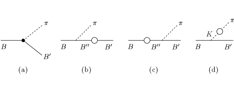
FIG. 1.: Diagrams contributing to the $P$-waves decays. Diagram (a) represents the contact contribution. Diagram (b)-(c) are the baryon pole contributions. Diagram (d) is the kaon pole contribution.

The contact contribution to the $P$-wave amplitude is obtained by replacing Eqs.(6, 14) in ${\cal L}_{w}$ and taking matrix elements of the terms proportional to $\partial_{\mu}\pi$. For example, for the amplitudes with $\pi_{0}$ emission one finds

$$B_{contact}(B\rightarrow B^{\prime}\pi_{0})=\frac{2(M_{B}+M_{B^{\prime}})}{3f_{\pi}}<\Psi_{B^{\prime}}|\left(I_{1}D_{63}+I_{2}D_{68}D_{33}+I_{3}D_{63}D_{38}\right)|\Psi_{B}>$$ (17)

where $M_{B}$ and $M_{B^{\prime}}$ are the masses of the initial and final baryons, respectively. $I_{1}$, $I_{2}$ and $I_{3}$ are radial integrals of rather involved functions of the soliton profile $F(r)$ which also depend on the constants $g$, $g^{\prime}$ and $g^{\prime\prime}$. Their explicit expressions can be found in Ref.[21].

On the other hand, the total pole term contribution to those processes is

$$B_{pole}(B\rightarrow B^{\prime}\pi_{0})={M_{B}+M_{B^{\prime}}\over{\sqrt{2}f_{\pi}}}\sum_{B^{\prime\prime}}\left[g_{A}^{B^{\prime}B^{\prime\prime}}\frac{A(B\rightarrow B^{\prime\prime}\pi_{0})}{M_{B}-M_{B^{\prime\prime}}}+g_{A}^{BB^{\prime}}\frac{A(B^{\prime\prime}\rightarrow B^{\prime}\pi_{0})}{M_{B^{\prime}}-M_{B^{\prime\prime}}}\right]$$ (18)

In deriving Eq.(18) we have dropped a negligible small $K$ pole term contribution (Fig.1d) and made use of the generalized Goldberger-Treiman relations to relate the strong coupling constants to the axial charge. In the present model the axial charge operator has been given in Ref.[22].

The numerical results for the $B$ amplitudes in which a neutral pion is emitted are given in Table 3. We observe that our predictions fail to reproduce the empirical decay amplitudes. The same happens for the charged pion amplitudes. In this sense, the situation is similar to that of other models such as quark models or heavy baryon chiral perturbation theory. For comparison some typical results of this latter approach are also listed in Table 3. They correspond to a lowest order chiral calculation. Next-to-leading order calculations do not improve the situation[9]. It is important to note that in our model the pole contributions are, in general, the result of a rather strong cancellation between the two (large) baryon pole contributions (Figs.1b-1c). Consequently, they appear to be very sensitive to the details of the model. In fact, something similar happens in the alternative baryon model calculations. As for the contact terms we observe that they are small and, therefore, do not contribute very much to explain the observed $P$-wave amplitudes.

V Conclusions

In this contribution we have presented some results for the radiative decay widths of the decuplet hyperons and the non-leptonic decay amplitudes of the octet hyperons in the context of the collective coordinate approach to the $SU(3)$ Skyrme model. We have found that, when normalized to that of the $\Delta N$ transition, the predictions for the radiative decay widths are qualitatively similar to those of alternative quark based models. On the other hand, the calculated $\Delta N$ transition amplitude turns to be roughly $30\%$ smaller than the empirical value. In the context of the $SU(2)$ Skyrme model it has been shown[17], however, that the inclusion of next-to-leading order quantum corrections solves this problem. In the $SU(3)$ model such corrections have been already included in the evaluation of the baryon masses[24] and corresponding results for the radiative decays widths will be available soon. In any case, it is important to stress that they are not expected to affect the ratios of decay amplitudes presented here. The situation concerning the non-leptonic weak hyperon decays is, unfortunately, not very satisfactory. Although we find that the model provides a rather good description of the empirical $S$-wave decay amplitudes, it fails to reproduce the observed $P$-wave ones. In particular, the contact contributions to the $P$-waves are not sufficient to explain the discrepancies between the pole contributions and the empirical values. Thus, in contrast to previous expectations[8, 10], within the present approximations the Skyrme model does not seem to provide a solution to the long-standing ’$S$-wave/$P$-wave puzzle’ which affects the available model calculations.

REFERENCES

- [1] T. H. R. Skyrme, Proc. R. Soc. London 260, 127 (1961); Nucl. Phys. 31 (1962) 556.
-
[2]
For reviews on the Skyrme model see:
G. Holzwarth and B. Schwesinger, Rep. Prog. Phys. 49 (1986) 82;
I. Zahed and G. E. Brown, Phys. Rep. 142 (1986) 481. - [3] H. Yabu and K. Ando, Nucl. Phys. B301 (1988) 601.
- [4] H. Weigel, Int. J. Mod. Phys A11 (1996) 2419.
- [5] R. A. Schumacher, Nucl. Phys. A585 (1995) 63c; Few Body Systems Supp. 11 (1999) 225.
- [6] J.W. Darewych, M. Horbatsch and R. Koniuk, Phys. Rev. D28 (1983) 1125.
- [7] D.B. Leinweber, T. Draper and R.M. Woloshyn, Phys. Rev. D48 (1993) 2230.
- [8] J.F. Donoghue, E. Golowich and B. R. Holstein, Phys. Rep. 131 (1986) 319.
- [9] E. Jenkins, Nucl. Phys. B375 (1992) 561, A. Abd El-hady and J. Tandean, hep-ph/9908498
- [10] J.F. Donoghue, E. Golowich and Y-C. R. Lin, Phys. Rev. D32 (1985) 1733; Erratum: Phys. Rev. D32 (1985) 1733.
- [11] M. Praszalowicz, Phys. Lett. 158B (1985) 264; M. Chemtob, Nucl. Phys. B256 (1985) 600.
- [12] M. Praszalowicz and J. Trampetic, Phys. Lett. 161B (1985) 169.
- [13] N.N. Scoccola, Phys. Lett. B428 (1998) 8.
- [14] E. Witten, Nucl. Phys. B223 (1983) 422; O. Kaymakcalan, S. Rajeev and J. Schechter, Phys. Rev. D30 (1984) 594.
- [15] T. Haberichter, H. Reinhardt, N.N. Scoccola and W. Weigel, Nucl. Phys. A615 (1997) 291.
- [16] H. Walliser and G. Holzwarth, Z. Phys. A357 (1997) 317.
- [17] F. Meier and H. Walliser, Phys. Rep. 289 (1997) 383.
- [18] J.F. Donoghue, E. Golowich and B. R. Holstein, Phys. Rev. D30 (1984) 587.
- [19] J. Kambor, J. Missimer and D. Wyler, Nucl. Phys. B346 (1990) 17.
- [20] J. Kambor, J. Missimer and D. Wyler, Phys. Lett. B261 (1991) 496.
- [21] A. Garcia, D. Gómez Dumm and N.N. Scoccola, in preparation.
- [22] N. W. Park, J. Schechter and H. Weigel, Phys. Rev. D43 (1991) 869.
- [23] J.F. Donoghue, E. Golowich and B. R. Holstein, Dynamics of the Standard Model (Cambridge Univ. Press, Cambridge, 1994)
- [24] H. Walliser, Phys. Lett. B432, 15 (1998); N.N. Scoccola and H. Walliser, Phys. Rev. D58, 094037 (1998).