Abstract

We present analytical next-to-leading order results for the correlator of baryonic currents at the three loop level with one finite mass quark. We obtain the massless and the HQET limit of the correlator from the general formula as particular cases. We also give explicit expressions for the moments of the spectral density.

Baryons are an important source of information on QCD interactions. Massive baryons containing a heavy quark form a rich family of particles with many properties experimentally measured [1]. The prominent object of a QCD analysis of the properties of baryons is the correlator of two baryonic currents and the spectral density associated with it. Calculations beyond the leading order have not been done for many interesting cases. The massless case has been known since long ago [2]. The mesonic analogue of our baryonic calculation was completed some time ago [3] and has subsequently provided a rich source of inspiration for many applications in meson physics.

We report on the results of calculating the $\alpha_{s}$ corrections to the correlator of two baryonic currents with one finite mass quark and two massless quarks. We give analytical results and discuss the order of magnitude of the $\alpha_{s}$ corrections. The massless and HQET limits are obtained as special cases. We finally present explicit results on the moments of the spectral density associated with the correlator. The discussion of the impact of our new correlator result on baryon phenomenology will be left to future publications.

In the present paper we limit ourselves to the simplest case with a three-quark current of the form

$$j=\epsilon^{abc}\Psi_{a}(u_{b}^{T}Cd_{c})$$ (1)

which has the quantum numbers of a $J^{P}=1/2^{-}$ baryon. $\Psi$ is a finite mass quark field with mass parameter $m$, $u$ and $d$ are massless quark fields, $C$ is the charge conjugation matrix, $\epsilon^{abc}$ is the totally antisymmetric tensor and $a,b,c$ are color indices for the $SU(3)$ color group. Other baryonic currents with any given specified quantum numbers are obtained from the current in Eq. (1) by inserting the appropriate Dirac matrices. Such additions introduce no principal complication into our method of calculation.

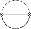
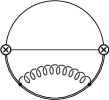
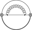
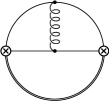
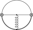
(a)(b)(c)(d)(e)

Figure 1: The calculated (a) two-loop and (b–e) three-loop topologies

The correlator of two baryonic currents is expanded as

$$i\int\langle Tj(x)\bar{j}(0)\rangle e^{iqx}dx=\gamma_{\nu}q^{\nu}\Pi_{q}(q^{2})+m\Pi_{m}(q^{2}).$$ (2)

For reasons of brevity we shall present results only for the invariant function $\Pi_{m}(q^{2})$. The invariant function $\Pi_{m}(q^{2})$ can be represented compactly via the dispersion relation

$$\Pi_{m}(q^{2})=\int_{m^{2}}^{\infty}\frac{\rho_{m}(s)ds}{s-q^{2}}$$ (3)

where $\rho_{m}(s)$ is the spectral density. All quantities are understood to be appropriately regularized. Since the spectral density is the real object of interest for phenomenological applications, we limit our subsequent discussion to the spectral density instead of the correlator. To simplify formulas we remove a trivial but awkward factor containing powers of $\pi$ and write

$$\rho_{m}(s)=\frac{1}{128\pi^{4}}\rho(s)$$ (4)

with a conveniently normalized $\rho(s)$,

$$\rho(s)=s^{2}\left\{\rho_{0}(s)\left(1+\frac{\alpha_{s}}{\pi}\ln\left(\frac{\mu^{2}}{m^{2}}\right)\right)+\frac{\alpha_{s}}{\pi}\rho_{1}(s)\right\}.$$ (5)

Here $\mu$ is the renormalization scale parameter, $m$ is a pole mass of the heavy quark (see e.g. [4]) and $\alpha_{s}=\alpha_{s}(\mu)$. The leading order two-loop contribution shown in Fig. 1(a) reads

$$\rho_{0}(s)=1+9z-9z^{2}-z^{3}+6z(1+z)\ln z$$ (6)

with $z=m^{2}/s$. In the $\overline{\rm MS}$-scheme the next-to-leading order three-loop contribution is given by

$$\rho_{1}(s)\ =\ 9+\frac{665}{9}z-\frac{665}{9}z^{2}-9z^{3}-\left(\frac{58}{9}+42z-42z^{2}-\frac{58}{9}z^{3}\right)\ln(1-z)$$ (7)

$$+\left(2+\frac{154}{3}z-\frac{22}{3}z^{2}-\frac{58}{9}z^{3}\right)\ln z+4\left(\frac{1}{3}+3z-3z^{2}-\frac{1}{3}z^{3}\right)\ln(1-z)\ln z$$

$$+12z\left(2+3z+\frac{1}{9}z^{2}\right)\left(\frac{1}{2}\ln^{2}z-\zeta(2)\right)+4\left(\frac{2}{3}+12z+3z^{2}-\frac{1}{3}z^{3}\right){\rm Li}_{2}(z)$$

$$+24z(1+z)\left({\rm Li}_{3}(z)-\zeta(3)-\frac{1}{3}{\rm Li}_{2}(z)\ln z\right)$$

where ${\rm Li}_{n}(z)$ are polylogarithms and $\zeta(n)$ is Riemann’s zeta function. The contributing three-loop diagrams are shown in Figs. 1(b) to (e). They have been evaluated using advanced algebraic methods for multi-loop calculations along the lines decribed in Refs. [5, 6]. For the convenience of the reader we briefly sketch our method of integration. All diagrams have first been reduced to scalar prototypes. The integrals over massless loops have been performed (for recurrent integration where possible) and one is left with the basic integral

$$V(\alpha,\beta;q^{2}/m^{2})=\int\frac{d^{D}k}{(k^{2}+m^{2})^{\alpha}(q-k)^{2\beta}}$$ (8)

which is a generalization of the standard object $G(\alpha,\beta)$ of the massless calculation. The integral $V$ is known analytically and suffices to calculate the diagrams in Fig. 1(c) and (d). For the calculation of the diagram shown in Fig. 1(e) the basic integral $V$ enters as a subdiagram. This subdiagram then is represented in terms of a dispersion integral which makes the whole diagram computable in terms of the same $V$ with the argument depending on the loop momentum. The final step is a finite range (convolution type) integration over this internal momentum with a spectral density of the basic integral $V$. The reduction to scalar prototypes of the diagram shown in Fig. 1(e) leads also to a new irreducible block (i.e. a prototype not expressible in terms of $V$) which is related to a two-loop master (fish) diagram. The result for this diagram is taken from Ref. [7].

The result presented in Eq. (7) is the main result of this paper: it represents the full next-to-leading order solution. Since the anomalous dimension of the current in Eq. (1) is known to two loop order [8], the result shown in Eq. (7) completes the ingredients necessary for an analysis of the scalar part of the correlator in Eq. (2) at the next-to-leading order level.

We now turn to the analysis of Eq. (7). Two limiting cases of interest are the near-threshold and high energy asymptotics. With our result given in Eq. (7) both limits can be taken explicitly. The asymptotic expressions can be also obtained in the framework of effective theories which can be viewed as special devices for such calculations.

In the high energy (small mass) limit $z\rightarrow 0$ the correction reads

$$\rho_{1}(s)=9+83z-4\pi^{2}z+2\ln z+50z\ln z+12z\ln^{2}z-24z\zeta(3)+O(z^{2}).$$ (9)

This will lead to the small mass expansion of the spectral density in the form

$$m\rho(s)=m_{\overline{\scriptstyle\rm MS}}(\mu)\rho^{\rm massless}(s)=m_{\overline{\scriptstyle\rm MS}}(\mu)s^{2}\left\{1+\frac{\alpha_{s}}{\pi}\left(2\ln\left(\frac{\mu^{2}}{s}\right)+\frac{31}{3}\right)\right\}$$ (10)

where $\rho^{\rm massless}(s)$ is the result of calculating the correlator in the effective theory of massless quarks. The relation between the pole (or invariant) mass parameter $m$ and the $\overline{\rm MS}$ mass $m_{\overline{\scriptstyle\rm MS}}(\mu)$ reads

$$m=m_{\overline{\scriptstyle\rm MS}}(\mu)\left\{1+\frac{\alpha_{s}}{\pi}\left(\ln\left(\frac{\mu^{2}}{m^{2}}\right)+\frac{4}{3}\right)\right\}.$$ (11)

Note that the massless effective theory cannot reproduce the mass singularities (terms like $z\ln(z)$ in Eq. (9)). The presence of these singularities is an infrared phenomenon and can be parametrized with condensates of local operators. In our case the first $m^{2}$ correction in Eq. (9) (and, of course, Eq. (6)) can be found if the perturbative value of the heavy quark condensate $\langle\bar{\Psi}\Psi\rangle$ taken from the full theory is added [9]. The composite operator $\langle\bar{\Psi}\Psi\rangle$ should be understood within a mass independent renormalization scheme such as the $\overline{\rm MS}$-scheme. This value (perturbatively, $\langle\bar{\Psi}\Psi\rangle\sim m^{3}\ln(\mu^{2}/m^{2})$) cannot be computed within the effective theory of massless quarks. It represents the proper matching between the perturbative expressions for the correlators of the full (massive) and effective (massless) theories. This matching procedure allows one to restore higher order terms of the mass expansion in the full theory from the effective massless theory with the mass term treated as a perturbation [10]. This is justified at high energies. Note that the correction to the next order (i.e. of order $m^{2}/s$) can actually be found in this manner because it depends only on one local operator and, therefore, the calculation is technically feasible.

In the near-threshold limit $E\rightarrow 0$ with $s=(m+E)^{2}$ one explicitly obtains

$$\rho^{\rm thr}(m,E)=\frac{16E^{5}}{5m}\bigg{\{}1+\frac{\alpha_{s}}{\pi}\ln\left(\frac{\mu^{2}}{m^{2}}\right)+\frac{\alpha_{s}}{\pi}\left(\frac{54}{5}+\frac{4\pi^{2}}{9}+4\ln\left(\frac{m}{2E}\right)\right)\bigg{\}}+O(E^{6}).$$ (12)

The invariant function $\rho_{m}$ suffices to determine the complete leading HQET behaviour since one has $q\kern-5.5pt/\rho_{q}+m\rho_{m}\rightarrow m(v\kern-5.0pt\raise 1.0pt\hbox{$\scriptstyle/$}\kern 1.0pt+1)\rho$ for the leading term. In this region the appropriate device to compute the limit of the correlator is HQET (see e.g. [11, 12]). Writing

$$m\rho^{\rm thr}(m,E)=C(m/\mu,\alpha_{s})^{2}\rho^{\rm HQET}(E,\mu)$$ (13)

we obtain the known result for $\rho^{\rm HQET}(E,\mu)$ [13] with matching coefficient $C(m/\mu,\alpha_{s})$ [14]. In this case the matching procedure allows one to restore the near-threshold limit of the full correlator starting from the simpler effective theory near threshold [15].

Note that the higher order corrections in $E/m$ to Eq. (12) can be easily obtained from the explicit result given in Eq. (7). Indeed, the next-to-leading order correction in low energy expansion reads

$$\Delta\rho^{\rm thr}(m,E)=-\frac{88E^{6}}{5m^{2}}\bigg{\{}1+\frac{\alpha_{s}}{\pi}\bigg{(}\ln\left(\frac{\mu^{2}}{m^{2}}\right)+\frac{376}{33}+\frac{4\pi^{2}}{9}+\frac{140}{33}\ln\left(\frac{m}{2E}\right)\bigg{)}\bigg{\}}.$$ (14)

It is a much more difficult task to obtain this result starting from HQET.

We now discuss some quantitative features of the correction given in Eq. (7). Of interest is whether the two limiting expressions (the massless limit expression as given in Eq. (10) and the HQET limit expression in Eqs. (12) and (13)) can be used to characterise the full function for all energies.

In Fig. 2 we compare components of the baryonic spectral function in leading and next-to-leading order. Shown is the ratio $\rho_{1}(s)/\rho_{0}(s)$. In the following we shall always put $\mu=m$ if it is not explicitly written. One can see that a simple interpolation between the two limits can give a rather good approximation for the next-to-leading order correction in the complete region of $s$.

Figure 2: The ratio $\rho_{1}(s)/\rho_{0}(s)$ of the next-to-leading correction and the leading order term in dependence of the energy square $s$

Another informative set of observables are moments of the spectral density

$${\cal M}_{n}=\int_{m^{2}}^{\infty}\frac{\rho(s)ds}{s^{n}}=m^{6-2n}M_{n}$$ (15)

with $M_{n}$ dimensionless. We find

$$M_{n}=M_{n}^{(0)}\left\{1+\frac{\alpha_{s}}{\pi}\left(\ln\left(\frac{\mu^{2}}{m^{2}}\right)+\delta_{n}\right)\right\}$$ (16)

where

$$M_{n}^{(0)}=\frac{12}{n(n-1)^{2}(n-2)^{2}(n-3)}$$ (17)

and

$$\delta_{n}=A_{n}+\frac{2\pi^{2}}{9}.$$ (18)

The coefficients $A_{n}$ are rational numbers. The closed form expression for the correction $\delta_{n}$ is long. Instead we present explicit expressions for the first several moments and the differences between consecutive moments in Table 1. We see that the difference between consecutive moments is reasonably small. The absolute value of the correction itself in the $\overline{\rm MS}$-scheme has no particular meaning and can be changed by modifying the subtraction scheme. In normalizing to a reference moment at $n=N$, the others can be expressed through

$$\frac{M_{n}}{M_{n}^{(0)}}=\frac{M_{N}}{M_{N}^{(0)}}\left\{1+\frac{\alpha_{s}}{\pi}(\delta_{n}-\delta_{N})\right\}.$$ (19)

One now can find the actual magnitude of the correction from Table 1. Indeed, for any given precision and range of $n$ the set of perturbatively commensurate moments can be found.

Note that moments represent massive vacuum bubbles, i.e. diagrams without external momenta with massive lines. These diagrams have been comprehensively analyzed in Refs. [16, 17]. The analytical results for the first few moments at three-loop level can be checked independently with existing computer programs (see e.g. [18]).

Moments of the spectral density are convenient observables for phenomenological applications. Exact results for correlators with massive particles are not known in higher orders for many important physical channels. Therefore one generally uses approximate procedures. We consider the two formal limiting cases as a base for possible interpolation. Both are simpler than the full calculation.

For the first approximation, the high energy or massless approximation, we first check the numerical difference between the exact result and the massless approximation. The massless limit for the moments means that one formally integrates the expression $\rho^{\rm massless}(s)$ in Eq. (10) over the range $(m^{2},\infty)$ to obtain

$${\cal M}_{n}^{\rm massless}=\int_{m^{2}}^{\infty}\frac{\rho^{\rm massless}(s)ds}{s^{n}}=m^{6-2n}M_{n}^{\rm massless}.$$ (20)

The result is

$$M_{n}^{\rm massless}=\frac{1}{n-3}\left\{1+\frac{\alpha_{s}}{\pi}\left(2\ln\left(\frac{\mu^{2}}{m^{2}}\right)+\frac{31}{3}-\frac{2}{n-3}\right)\right\}.$$ (21)

This is the extrapolation from the side of high energies. The opposite limit for the moments is obtained by using the near-threshold spectral density for the integration along the whole $s$-axis. This approximation is an extrapolation from the threshold region which is clearly a poor approximation far from threshold. However, it formally exists for sufficiently large $n$ and can be obtained with the simple HQET result shown in Eqs. (12) and (13). The moments are given by

$$M_{n}^{\rm thr}=m^{2n-6}\int_{m^{2}}^{\infty}\frac{\rho^{\rm thr}(E)ds}{s^{n}}=2m^{2n-6}\int_{0}^{\infty}\frac{\rho^{\rm thr}(E)dE}{(m+E)^{2n-1}}.$$ (22)

From Eq. (12) we have

$$M_{n}^{{\rm thr}(0)}=12\frac{2^{6}(2n-8)!}{(2n-2)!}=\frac{12}{n^{6}}\left(1+O(n^{-1})\right)$$ (23)

where the large $n$ result specifies the region of applicability of the near-threshold approximation for the moments of the spectral density. The correction is

$$M_{n}^{\rm thr}=M_{n}^{{\rm thr}(0)}\bigg{\{}1+\frac{\alpha_{s}}{\pi}\bigg{(}\ln\left(\frac{\mu^{2}}{m^{2}}\right)+\frac{54}{5}+\frac{4\pi^{2}}{9}-4\ln 2-4(\psi(2n-7)-\psi(6))\bigg{)}\bigg{\}}$$ (24)

where $\psi(z)$ is Euler’s $\psi$-function.

One can see that the corrections to the moments basically reflect the shape of the correction to the spectrum as given in Eq. (7). The massless approximation is reasonably good for relative corrections for the first few moments despite the unfavorable shape of the weight function $1/s^{n}$. It can be improved by changing the subtraction point $\mu$ or by resumming the integrand [19] which lies beyond the scope of finite order perturbation theory though.

To conclude, we have computed the next-to-leading perturbative corrections to the finite mass baryon correlator at three-loop order. Technically, the method allows one to obtain analytical results for two-point correlators of composite operators with one finite mass particle which can be compared to HQET results. Corrections in $E/m$ near threshold are easily available from our explicit results. From threshold to high energies the exact spectral density interpolates nicely between the leading order HQET result close to threshold and the asymptotic mass zero result. Going even one order higher it is very likely that the full four-loop spectral density can be well approximated by the corresponding massless four-loop result which can be calculated using existing computational algorithms [20, 21].

$n$	$A_{n}$	$\delta_{n}-\delta_{n-1}$
4	3
5	13/2	3.500000
6	17/2	2.000000
7	535/54	1.407407
8	1187/108	1.083333
9	64093/5400	0.878333
10	22691/1800	0.737037
11	1167767/88200	0.633878
12	2433499/176400	0.555357
13	68055703/4762800	0.493665
14	14034047/952560	0.443968
15	348916495/23051952	0.403114
16	8935543717/576298800	0.368960
17	3086442535481/194788994400	0.340003
18	3147830736641/194788994400	0.315152
19	3205021446217/194788994400	0.293603
20	6517078055669/389577988800	0.274746
21	382499185005589/22517607752640	0.258112

Table 1: Values for the rational part $A_{n}$ of the first moments $\delta_{n}$ and their relative difference $\delta_{n}-\delta_{n-1}$

References

- [1] Particle Data Group, Eur. Phys. J. C3 (1998) 1
- [2] A.A. Ovchinnikov, A.A. Pivovarov and L.R. Surguladze, Sov. J. Nucl. Phys. 48 (1988) 358; Int. J. Mod. Phys. A6 (1991) 2025
- [3] S.C. Generalis, Report No. OUT-4102-13 (1984), later published as J. Phys. G16 (1990) 367, see also D.J. Broadhurst, Phys. Lett. 101 B (1981) 423; D.J. Broadhurst and S.C. Generalis, Report No. OUT-4102-8/R (1982)
- [4] R. Tarrach, Nucl. Phys. B183 (1981) 384
- [5] S. Groote, J.G. Körner and A.A. Pivovarov, Nucl. Phys. B542 (1999) 515
- [6] S. Groote, J.G. Körner and A.A. Pivovarov, Phys. Rev. D60 (1999) 061701
- [7] D.J. Broadhurst, Z. Phys. C47 (1990) 115
- [8] A.A. Pivovarov and L.R. Surguladze, Nucl. Phys. B360 (1991) 97
- [9] H.D. Politzer, Nucl Phys. B117 (1976) 397
- [10] V.P. Spiridonov and K.G. Chetyrkin, Sov. J. Nucl. Phys. 47 (1988) 522
- [11] H. Georgi, Nucl. Phys. B363 (1991) 301
- [12] M. Neubert, Phys. Rep. 245 (1994) 259
- [13] S. Groote, J.G. Körner and O.I. Yakovlev, Phys. Rev. D55 (1997) 3016
- [14] A.G. Grozin and O.I. Yakovlev, Phys. Lett. 285 B (1992) 254
- [15] E. Eichten and B. Hill, Phys. Lett. 234 B (1990) 511
- [16] L.V. Avdeev, Comput. Phys. Commun. 98 (1996) 15
- [17] D.J. Broadhurst, Eur. Phys. J. C8 (1999) 311
- [18] K.G. Chetyrkin, J.H. Kühn and M. Steinhauser, Nucl. Phys. B505 (1997) 40
-
[19]
A.A. Pivovarov, Sov. J. Nucl. Phys. 54 (1991) 676;
Z. Phys. C53 (1992) 461; Nuovo Cim. 105 A (1992) 813 -
[20]
K.G. Chetyrkin and F.V. Tkachov,
Nucl. Phys. B192 (1981) 159;
F.V. Tkachov, Phys. Lett. 100 B (1981) 65 - [21] K.G. Chetyrkin and V.A. Smirnov, Phys. Lett. 144 B (1984) 419