Scheme Dependence of Weak Matrix Elements in the $1/N_{c}$ Expansion

Abstract:

We show how the scheme- and scale-dependence of the short-distance operator product expansion with four-quark operators can be correctly accounted for in the framework of the $1/N_{c}$-expansion once the hadronization of two-quark currents has been fixed. We show formulas explicitly in the case of the $B_{K}$-parameter. We then use them with our earlier estimates of the long-distance effects. We compare Chiral Perturbation Theory at Leading- and Next-to-Leading-Order with the ENJL model results in the chiral limit. Good matching between the long- and short-distance regimes is obtained and our final value for the physical scheme independent $\hat{B}_{K}$ is $0.77\pm 0.05\pm 0.05$.

1 Introduction

Weak non-leptonic decays and mixings are one of our few windows on the CP-violating sector of the Standard Model and their calculation is thus important. A set of reviews summarizing the present status in the kaon area can be found in the various talks at the workshops at Orsay and Chicago[1, 2].

The large difference in mass between the $W$-boson and the kaon presents an additional difficulty since logarithms of this ratio need to be summed to all orders. This can be done using the Operator Product Expansion (OPE) and is by now standard. The remaining problem is the calculation of the matrix elements of these operators at some low scale.

That the $1/N_{c}$-expansion would be useful in this regards was first suggested by Bardeen, Buras, and Gérard[3, 4] and has been reviewed recently by Bardeen[5]. There one can find most of the references to previous work and applications of this non-perturbative technique.

Since the original work[3] there are have been some improvements. This has centered on identifying more correctly the scales in short- and long-distance[6, 7] and their matching. A more precise method to perform this identification was proposed in [8], the $X$-boson method, and shown there to provide a correct matching with the renormalization group evolution at one-loop. At next-to-leading (NLO) in the renormalization group running several other problems appear. The operators become scheme dependent and also dependent on various other choices like the one of evanescent operators. This is discussed in the review by Buras[9] and also in the original OPE at NLO papers[10, 11].

In this paper we show how scheme and scale dependence can consistently be treated within the $1/N_{c}$-expansion technique as argued in [4, 5, 12, 13]. We will use the method suggested in [8] as already used in [12, 13]. In particular we will show explicit expressions for the current $\times$ current $\Delta S=2$ four-quark operator in the Standard Model. In practice this means tracking the scheme dependence consistently during the entire calculation.

We are concerned here with the short-distance matching between the definition of the weak operators done in perturbative QCD using a particular regularization scheme and the actual calculation of weak matrix elements at a given order in the $1/N_{c}$ expansion. This can be done purely within perturbation theory and is unambiguous once the short-distance schemes used in perturbative QCD are specified. We will also show explicitly that it does not depend on the infrared regulators. We then use this result together with the matrix element obtained earlier in [12] to obtain complete scheme-independent results for the $\hat{B}_{K}$ parameter within the $1/N_{c}$ expansion. We also discuss the long-distance short-distance matching for this quantity.

2 The Flavour Changing Effective Action and the $X$-Boson Method

In light hadrons flavour changing decays there appear two very different scales; namely, the hadronic scale and the weak scale, which makes necessary the use of effective field theory analyses. This is done with the help of the OPE which allows to separate short-distance from long-distance physics. The OPE analysis is done at some scale below the $W$ mass and this separation introduces some short-distance scale and regulator scheme dependence which has to cancel in the final physical amplitude. We will see how this occurs explicitly in the $1/N_{c}$ technique.

The process of obtaining the relevant effective action continues by integrating out the heavy degrees of freedom up to some scale below the charm quark mass and setting the appropriate matching conditions at heavy particle thresholds [9]. This can be done using QCD perturbation theory. In this process, large logarithms $\left(\alpha_{s}(\nu)\ln(M_{W}/\nu)\right)^{k}$ need to be resummed to all orders in perturbation theory. This is done with the help of Renormalization Group (RG) techniques which at Next-to-Leading-Log-Order (NLLO) allow to resum up to $\alpha_{s}(\nu)\,\left(\alpha_{s}(\nu)\ln(M_{W}/\nu)\right)^{k}$. In fact, only from NLLO can a full scheme dependence study be done.

The whole process described schematically above is by now standard and has been brought up to NLLO in [10, 11] from the earlier Leading-Log-Order (LLO) results[14]. For comprehensive reviews where complete details can be found, see [9].

Thus, at some scale $\nu$ below the charm quark mass, we are left with the effective field theory action

$$\Gamma_{\Delta S=a}\equiv-C_{\Delta S=a}{\displaystyle\sum_{i}}\,C_{i}(\nu)\int{\rm d}^{4}\,y\,\,Q_{i}(y)+{\rm h.c.}$$ (1)

to describe hadronic flavour changing processes in the Standard Model. Here $Q_{i}(x)$ is the set of four-quark operators made out of the three light-quark fields. They change flavour in $a$ units and are defined perturbatively within QCD using some regularization. In particular, the NLLO calculations mentioned above have been done both in the ’t Hooft-Veltman (HV) scheme ($\overline{\rm MS}$ subtraction and non-anti-commuting $\gamma_{5}$ in $D\neq 4$) and in the Naive Dimensional Regularization (NDR) scheme ($\overline{\rm MS}$ subtraction and anti-commuting $\gamma_{5}$ in $D\neq 4$).

In order to reach a physical process we now need to calculate matrix elements of the effective action (1) between the physical states. In this calculation, all dependence on the different schemes used and on the scale $\nu$ should disappear. This necessarily involves long-distances which cannot be treated analytically within QCD. One option is to simply give up here and refer to lattice QCD calculations. However, these have at present many problems with this type of matrix elements. They are complicated quantities to treat on the lattice and chiral symmetry effects are very important. For a recent review on lattice QCD weak hadronic matrix elements see e.g. [15]. Here we would like to show how to connect the effective action in a well defined way with other approaches to low-energy QCD.

To identify a four-quark operator in any model or approximation to QCD like e.g. Chiral Perturbation Theory (CHPT), is very difficult. On the other hand, all these approximations and models are normally tuned to reproduce various experimentally observed properties involving currents and/or made to specifically match perturbative QCD predictions for Green functions involving currents. As a rule therefore, identification of two-quark currents is possible. So a first step is to replace $\Gamma_{\Delta S=a}$ by an equivalent effective action that only involves currents.

We thus introduce an action of $X$-bosons with masses $M_{X}$ coupling to quark currents, whose OPE reproduces Eq. (1). This requirement fixes the couplings of the $X$-bosons. This matching can be done at a perturbative level in QCD with external states consisting of quarks and gluons as long as the scale $\nu$ is high enough. At this matching the scale and scheme-dependence of Eq. (1) has disappeared and, as we show below, the $X$-boson couplings are independent of the precise infrared regulator chosen here.

We now split the integral over $X$-boson momenta into two parts. The high energy part needs to have the momentum flow back through perturbative quarks and gluons leaving an operator behind that only needs to be evaluated to leading order in $1/N_{c}$. The low energy part needs to be evaluated using the $1/N_{c}$ method to NLO in $1/N_{c}$. Putting the two parts together we can see that all dependence on the $X$-boson masses has dropped out and the final result can be written in a way that only involves the coefficients of the operators in Eq. (1) with the scheme dependence removed correctly. In the next section, we will show this procedure explicitly for the $\Delta S=2$ four-quark operator. The same procedure can be worked out for the $\Delta S=1$ effective action but is much more cumbersome[16].

3 The $\Delta S=2$ Case

We present a complete analysis for the $\Delta S=2$ case. The generalization to other flavour changing processes is straightforward. The Standard Model effective action for $\Delta S=2$ transitions is

$$\Gamma_{\Delta S=2}\equiv-C_{\Delta S=2}\,C(\nu)\,\int{\rm d}^{4}\,y\,\,Q_{\Delta S=2}(y)+{\rm h.c.}$$ (2)

with

$$Q_{\Delta S=2}(x)\equiv 4L^{\mu}(x)L_{\mu}(x)\,;{\hskip 14.22636pt}2L^{\mu}\equiv\left[\overline{s}\gamma^{\mu}\left(1-\gamma_{5}\right)d\right](x)\,.$$ (3)

The operator $Q_{\Delta S=2}$ transforms under SU(3)_L $\times$ SU(3)_R rotations as a 27_L $\times$ 1_R. The normalization factor

$$C_{\Delta S=2}\equiv\frac{G_{F}}{4}{\cal F}(m_{t}^{2},m_{c}^{2},M_{W}^{2},V_{CKM})$$ (4)

is a known function of the integrated out heavy particles masses and Cabibbo-Kobayashi-Maskawa matrix elements and the Wilson coefficient $C(\nu)$ is known to NLLO[11].

The $\Delta S=2$ $K^{0}$-$\overline{K^{0}}$ matrix element

$$\langle\overline{K^{0}}|K^{0}\rangle\equiv-i\,C_{\Delta S=2}\,C(\nu)\langle\overline{K^{0}}|\int{\rm d}^{4}\,y\,\,Q_{\Delta S=2}(y)|K^{0}\rangle\,$$ (5)

governs the short-distance contribution to the $K_{L}$-$K_{S}$ mixing. We describe now how to calculate it in the $1/N_{c}$ expansion [3, 8, 12, 17].

3.1 Transition to $X$-boson Effective Theory

First of all, we need to set the matching conditions between the weak operator $Q_{\Delta S=2}$ defined by (3) and the short-distance part of the effective field theory of $X$-bosons used in the $1/N_{c}$ technique. The effective action of the latter is

$$\Gamma_{X}\equiv 2g_{\Delta S=2}(\mu_{C},M_{X},\cdots)\,\int{\rm d}^{4}y\,X^{\mu}(y)\,L_{\mu}(y)+{\rm h.c.}\,$$ (6)

where $g_{\Delta S=2}(\mu_{C},M_{X},\cdots)$ is an effective coupling. In addition we add kinetic and mass terms for the $X$-bosons. Evaluating matrix elements of $\Gamma_{\Delta S=2}$ needs to be done in the scheme in which it is defined. We can freely choose the scheme in which we should treat $\Gamma_{X}$. Here we choose an Euclidean cut-off regulator with subtraction to define the strong coupling $\alpha_{s}$ at a scale $\mu_{C}$. This has certain advantages for the next subsection.

We now determine the coupling $g_{\Delta S=2}$ by requiring that the matrix elements of $\Gamma_{\Delta S=2}$ are the same as those of $\Gamma_{X}$ to leading order in $1/M_{X}$. We require at some perturbative scale

$$\langle s(q_{1})\overline{d}(q_{4})|e^{i\Gamma_{\Delta S=2}}|\overline{s}(q_{2})d(q_{3})\rangle=\langle s(q_{1})\overline{d}(q_{4})|e^{i\Gamma_{X}}|\overline{s}(q_{2})d(q_{3})\rangle+{\cal O}(1/M_{X}^{4})\;.$$ (7)

Where we have taken the matrix elements between an incoming strange anti-quark with momentum $q_{2}$ and an incoming down quark with momentum $q_{3}$ and an outgoing strange quark with momentum $q_{1}$ and an outgoing down anti-quark with momentum $q_{4}$. We regulate infrared divergences by having $-q_{i}^{2}>0$. In order to have expressions of manageable length we require $-q_{i}^{2}\ll|q_{i}\cdot q_{j\neq i}|\ll\mu_{C}^{2},\nu^{2},M_{X}^{2}$ but we have kept all momenta different in order to show the full cancellation and remove any possible ambiguities in applying the equations of motion.

Both sides in (7) are by themselves scale, scheme, and regulator independent at at given order. This is to order $\alpha_{s}^{2}(\nu)$ if we use NLLO results. They do depend on the infrared regulators used, like the quark momenta, and the gluon gauge but these are the same in both sides and cancel in the matching. The gauge dependence we discuss in Section 3.3.

The left-hand side of (7) evaluated at NLLO using the diagrams of Figure 1

Figure 1: The type of diagrams contributing to the matrix element of $\Gamma_{\Delta S=2}$. The circle denotes the current-current operator. Colours are connected on the same side of the horizontal line. The curly line is a gluon and full lines are quarks. (a) Wave Function Renormalization. (b) Vertex Diagrams. (c)(d) Box Diagrams.

is

$$iC_{D}\,\left[\left(1+F(q_{1},q_{2},q_{3},q_{4})\frac{\alpha_{s}(\nu)}{\pi}\right)S_{1}+\left(1+F(q_{1},q_{2},-q_{4},-q_{3})\frac{\alpha_{s}(\nu)}{\pi}\right)S_{2}\right]$$ (8)

with

$$C_{D}=-C_{\Delta S=2}\,C(\nu)\left(1+\frac{\alpha_{s}(\nu)}{\pi}\left[\frac{\gamma_{1}}{2}\ln\left(\frac{2q_{1}.q_{2}}{\nu^{2}}\right)+r_{1}\right]\right)$$ (9)

where $\nu$ is a scale where perturbative QCD can be used. The function

$$F(q_{1},q_{2},q_{3},q_{4})=B(q_{1},q_{2},q_{3},q_{4})-\frac{1}{N_{c}}B(q_{1},q_{2},-q_{4},-q_{3})+\frac{N_{c}^{2}-1}{2N_{c}}V(q_{1},q_{2},q_{3},q_{4})\,;$$ (10)

collects finite terms from the box (B) and vertex diagrams (V).

$$S_{1} = \left[\overline{s}_{1}\gamma_{\mu}(1-\gamma_{5})d_{3}\right]\left[\overline{s}_{2}\gamma^{\mu}(1-\gamma_{5})d_{4}\right]$$

$$S_{2} = \left[\overline{s}_{1}\gamma_{\mu}(1-\gamma_{5})d_{4}\right]\left[\overline{s}_{2}\gamma^{\mu}(1-\gamma_{5})d_{3}\right]$$ (11)

are tree level matrix elements. The colour indices are summed inside brackets. The $\Psi_{i}$ field destroys a quark $\Psi$ with momentum $q_{i}$. In the NDR scheme, using the Feynman gauge for the gluon, the one-loop anomalous dimensions is

$$\gamma_{1}=\frac{3}{2}\left(1-\frac{1}{N_{c}}\right)$$ (12)

and

$$r_{1}^{NDR}=-\frac{9}{4}\left(1-\frac{1}{N_{c}}\right)\,.$$ (13)

The one-loop anomalous dimensions $\gamma_{1}$ is scheme-independent and

$$r_{1}^{HV}=-\frac{7}{4}\left(1-\frac{1}{N_{c}}\right)\,.$$ (14)

if we use the ’t Hooft-Veltman scheme instead. In both cases we have used the same scheme for the evanescent operators as the one in [11, 18].

The terms with $F(q_{1},q_{2},q_{3},q_{4})$ collect the infrared dependence on quark masses, external quark momenta, $\cdots$ as well as scheme-independent constants. If we had used a gluon mass as infrared regulator that would have been present there as well. The separation of the constant terms between $r_{1}$ and $F(q_{1},q_{2},q_{3},q_{4})$ is arbitrary.

The explicit expression for the box function $B(q_{1},q_{2},q_{3},q_{4})$ is

$$B(q_{1},q_{2},q_{3},q_{4}) = \frac{1}{4}\left[\ln\left(\frac{-2q_{3}\cdot q_{4}}{q_{3}^{2}}\right)\ln\left(\frac{-2q_{3}\cdot q_{4}}{q_{4}^{2}}\right)+\ln\left(\frac{-2q_{1}\cdot q_{2}}{q_{1}^{2}}\right)\ln\left(\frac{-2q_{1}\cdot q_{2}}{q_{2}^{2}}\right)\right.$$ (15)

$$- \ln\left(\frac{-2q_{1}\cdot q_{3}}{q_{1}^{2}}\right)\ln\left(\frac{-2q_{1}\cdot q_{3}}{q_{3}^{2}}\right)-\ln\left(\frac{-2q_{2}\cdot q_{4}}{q_{2}^{2}}\right)\ln\left(\frac{-2q_{2}\cdot q_{4}}{q_{4}^{2}}\right)$$

$$+ \left.\frac{1}{2}\ln\left(\frac{q_{1}\cdot q_{3}}{q_{1}\cdot q_{2}}\right)+\frac{1}{2}\ln\left(\frac{q_{2}\cdot q_{4}}{q_{1}\cdot q_{2}}\right)\right]+{\cal O}(q_{i}^{2}/(q_{j}\cdot q_{k\neq j}))$$

and for the vertex function $V(q_{1},q_{2},q_{3},q_{4})$ is

$$V(q_{1},q_{2},q_{3},q_{4}) = -\frac{1}{4}\left[2+\frac{4\pi^{2}}{3}+2\ln\left(\frac{-2q_{1}\cdot q_{3}}{q_{1}^{2}}\right)\ln\left(\frac{-2q_{1}\cdot q_{3}}{q_{3}^{2}}\right)\right.$$ (16)

$$+ \left.2\ln\left(\frac{-2q_{2}\cdot q_{4}}{q_{2}^{2}}\right)\ln\left(\frac{-2q_{2}\cdot q_{4}}{q_{4}^{2}}\right)-\frac{3}{2}\ln\left(\frac{-2q_{1}\cdot q_{3}}{q_{1}^{2}}\right)-\frac{3}{2}\ln\left(\frac{-2q_{1}\cdot q_{3}}{q_{3}^{2}}\right)\right.$$

$$- \left.\frac{3}{2}\ln\left(\frac{-2q_{2}\cdot q_{4}}{q_{2}^{2}}\right)-\frac{3}{2}\ln\left(\frac{-2q_{2}\cdot q_{4}}{q_{4}^{2}}\right)\right]+{\cal O}(q_{i}^{2}/(q_{j}\cdot q_{k\neq j}))\;.$$

In the HV scheme one gets the same expressions for these two functions.

The Wilson coefficient $C(\nu)$ at NNLO can be written as

$$C(\nu) = \left(1+\frac{\alpha_{s}(\nu)}{\pi}\left[\frac{\gamma_{2}}{\beta_{1}}-\frac{\beta_{2}\gamma_{1}}{\beta_{1}^{2}}\right]\right)\left[\alpha_{s}(\nu)\right]^{\gamma_{1}/\beta_{1}}$$ (17)

with [11]

$$\gamma_{2}^{\rm NDR} = \frac{1}{32}\left(1-\frac{1}{N_{c}}\right)\,\left[-17+4(n_{f}-3)+\frac{57}{N_{c}}\left(1-\frac{N_{c}^{2}}{9}\right)\right]$$

$$\gamma_{2}^{\rm HV} = \frac{1}{32}\left(1-\frac{1}{N_{c}}\right)\,\left[-17+4(n_{f}-3)+\frac{57}{N_{c}}\left(1-\frac{N_{c}^{2}}{9}\right)-16\beta_{1}\right]$$ (18)

with $\beta_{1}=-9/2$ and $\beta_{2}=-8$. The Feynman gauge for the gluon has been used to obtain the results above [11]. The scheme of evanescent operators we used is the one of [11, 18].

Equation (8) is now scheme-independent and scale-independent to order $\alpha_{s}^{2}$, the difference in running via Eq. (3.1) is compensated by the difference between (13) and (14). This was shown with simpler states also in [18]. We can now check this by plotting $-C_{D}/C_{\Delta S=2}$ versus $\nu$ for the two schemes. The difference and the variation with $\nu$ is an indication of the neglected $\alpha_{s}^{2}$ corrections. This is shown in Figure 2 where we plot the one-loop coefficient $C(\nu)$ and the two-loop one for both the NDR and the HV schemes. They differ considerably and are rather $\nu$-dependent. Now $-C_{D}/C_{\Delta S=2}$ of Eq. (9) is more stable with $\nu$ and has a smaller scheme-dependence left. Both are an indication of the size of the $\alpha_{s}^{2}$ corrections. This can be improved systematically by doing the matching to order $\alpha_{s}^{2}$ and the running to three-loops and so on. We have chosen $2q_{1}\cdot q_{2}=1$ GeV² and $\alpha_{s}(M_{\tau})=0.334$ [22] as input.

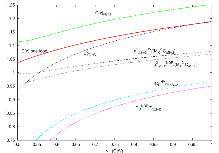
Figure 2: The short-distance coefficients.

For the left-hand side of (7) we need to specify now which is the effective field theory we use in the $1/N_{c}$ calculation. We introduced a fictitious [4, 8] $X^{\mu}$ boson which reproduces the physics of the $Q_{\Delta S=2}(x)$ weak operator below $\mu_{C}\approx\nu$, with coupling given in $\Gamma_{X}$ of Eq. (6).

For the right-hand side of (7) at NLLO we get

Figure 3: The type of diagrams contributing to the matrix element of $X$-boson exchange. The wiggly line is the $X$-boson, the curly line is a gluon and full lines are quarks. (a) Wave Function Renormalization. (b) Vertex Diagrams. (c)(d) Box Diagrams.

$$iC_{C} \left[\left(1+F(q_{1},q_{2},q_{3},q_{4})\frac{\alpha_{s}(\mu_{C})}{\pi}\right)S_{1}+\left(1+F(q_{1},q_{2},-q_{4},-q_{3})\frac{\alpha_{s}(\mu_{C})}{\pi}\right)S_{2}\right]$$ (19)

$$+{\cal O}\left(\frac{1}{M_{X}^{4}}\right)$$

using the diagrams of Figure 3, with

$$C_{C}\equiv\frac{-g_{\Delta S=2}^{2}}{M_{X}^{2}}\left(1+\frac{\alpha_{s}(\mu_{C})}{\pi}\left[\frac{\gamma_{1}}{2}\ln\left(\frac{2q_{1}.q_{2}}{M_{X}^{2}}\right)+\tilde{r}_{1}\right]\right)\;.$$ (20)

We have used the conditions in the $X$-boson effective theory $M_{X}^{2}\gg q_{i}^{2}$ and $\mu_{C}^{2}\gg-q_{i}^{2}$. For the scheme dependent constant we get

$$\tilde{r}_{1}=-\frac{7}{8}\left(1-\frac{1}{N_{c}}\right)\,.$$ (21)

The box diagrams are finite in this case, the only divergent ones are the vertex and wave-function renormalization diagrams, (a) and (b) in Figure 3.

The expression in (19) is also scale- and scheme-independent at order $\alpha_{s}^{2}$. The constant $\tilde{r}_{1}$ is scheme dependent but it cancels against the same dependence in the constant $g_{\Delta S=2}$.

About the QCD regularization used, notice that there are no logarithms depending on the scale $\mu_{C}$. This is not trivial, in principle these can also appear. This is a consequence of the fact that the anomalous dimension vanishes for two-quark vector and axial-vector currents and that box diagrams are finite. Two-quark currents can be identified always in the low-energy approximation to QCD unambiguously as said before. And for box diagrams we can use $D=4$ and therefore their contribution is $\gamma_{5}$ and evanescent operator schemes independent.

The infrared regulator scheme dependence is , as it should be, precisely the same in Eq. (8) and (19), precisely the same function $F(q_{1},q_{2},q_{3},q_{4})$ appears.

The $X$ boson mass acts here like an ultraviolet regulator. The dependence has to disappear in the final physical amplitude. We will see how this happens in the matching between long- and short-distances.

So from the matching condition in (7) we obtain for the $X$-boson couplings:

$$g^{2}_{\Delta S=2}(\mu_{C},M_{X},\cdots) = M_{X}^{2}C_{\Delta S=2}C(\nu)\Bigg{(}1+\frac{\alpha_{s}(\nu)}{\pi}\left[\gamma_{1}\ln\frac{M_{X}}{\nu}+r_{1}-\tilde{r}_{1}\right]$$ (22)

$$+ {\cal O}\left(\alpha_{s}^{2}(\mu_{C}),\alpha_{s}^{2}(\nu),\alpha_{s}(\nu)-\alpha_{s}(\mu_{C})\right)\Bigg{)}\,.$$

and $\alpha_{s}(\nu)-\alpha_{s}(\mu_{C})$ is also of order $\alpha_{s}^{2}$. We also plotted $-g^{2}_{\Delta S=2}/(M_{X}^{2}C_{\Delta S=2})$ in Figure 2 to show the effect of $\tilde{r}_{1}$ for the HV and NDR schemes. Again we see that the result is stable with $\nu$. We used $M_{X}=1$ GeV for definiteness.

With this first matching we have obtained an expression which is scale and scheme independent to NLLO order. In addition in the $X$-boson theory the only part that needs regularization is the $X$-boson–quark vertex itself and we have not used any $1/N_{c}$ argument until now.

3.2 Long-Distance Short-Distance Matching and $1/N_{c}$

With the value of $g_{\Delta S=2}$ set in (22) we can calculate the weak matrix element in the $1/N_{c}$ expansion within the $X$-boson exchange effective theory.

We follow the same technique we used for calculating the electromagnetic mass difference for pions and kaons in [19] and related work can be found in [6, 20, 21]. We obtained very nice matching for four-point functions in the presence of quark masses. At present, this non-trivial matching has only been obtained in the $1/N_{c}$-technique.

A point we do not discuss here is the choice of gauge for the $X$-boson. For reasonable gauges the effect are suppressed by extra powers of $1/M_{X}^{2}$ so they are not needed here. In any case the discussion for the photon in [19] can be easily extended to show that there is no problem here in general either.

We want to calculate some matrix element between hadronic states in general. For our example in (5):

$$\langle\overline{K^{0}}|K^{0}\rangle=\langle\overline{K^{0}}|e^{i\Gamma_{\Delta S=2}}|K^{0}\rangle=\langle\overline{K^{0}}|e^{i\Gamma_{X}}|K^{0}\rangle$$ (23)

$$= -\frac{g_{\Delta S=2}^{2}}{2}\langle\overline{K^{0}}|\int{\rm d}^{4}x\,\int{\rm d}^{4}y\,4L^{\mu}(x)L_{\mu}(y)P_{X}(x,y)|K^{0}>\,.$$

The equality follows from the discussion in the previous subsection. $P_{X}(x,y)$ is the $X$-boson propagator

$$P_{X}(x,y)=\int\frac{d^{4}p_{X}}{(2\pi)^{4}}\frac{i}{p_{X}^{2}-M_{X}^{2}}e^{-i(x-y)\cdot p_{X}}\;.$$ (24)

The matrix element corresponds to a four-quark operator in an OPE in the $X$-boson effective theory.

We now rotate the integral in (24) into the Euclidean and split the integral into two parts $|p_{E}|>\mu$ and $|p_{E}|<\mu$. One of the reasons to rotate to Euclidean space is that in the lower part then all components of $p_{E}$ are also small. Also, in general, amplitudes are much smoother in the Euclidean region, so approximations are generally better behaved since threshold effects and the like are smeared out. In particular we split

$$\int{\rm d}^{4}p_{E}=\int d\Omega_{p_{E}}\;\Bigg{(}\underbrace{\int_{0}^{\mu}{\rm d}|p_{E}|\,|p_{E}|^{3}}_{\mbox{long-distance}}+\underbrace{\int_{\mu}^{\infty}{\rm d}|p_{E}|\,|p_{E}|^{3}}_{\mbox{short-distance}}\Bigg{)}\;.$$ (25)

This is the same procedure as applied to the electromagnetic mass difference of pions and kaons in [19]. We choose $M_{X}\gg\mu$ such that in the long-distance part we can neglect all momentum dependence of the $X$-propagator and we expand the short-distance part in $1/M_{X}^{2}$.

Form-factors of mesons at large Euclidean momenta $p_{E}^{2}$ are suppressed by $1/p_{E}^{2}$, so in the short-distance part the high momentum has to flow back through quarks and gluons to leading order in $1/\mu^{2}$. The short-distance part is a two-step calculation, we evaluate the the integral with the momentum flowing back through gluons and quarks using the box diagrams of Figure 3 only. The vertex diagrams do not involve a large $X$-boson momentum so they are part of the long-distance calculation. Here there is no infrared ambiguity, the possible infrared divergence is regulated by $\mu$, the lower limit of the short-distance integral. The result is:

$$\langle\overline{K^{0}}|{K^{0}}\rangle_{SD\mbox{-}X}=\frac{-ig_{\Delta S=2}^{2}}{2M_{X}^{2}}\langle\overline{K^{0}}|S_{1}+S_{2}|K^{0}\rangle\frac{\alpha_{s}(\mu)}{\pi}\gamma_{1}\ln\frac{\mu}{M_{X}}\,.$$ (26)

Here $\alpha_{s}$ is already suppressed by $1/N_{c}$ so it is sufficient to calculate $\langle\overline{K^{0}}|S_{1}+S_{2}|K^{0}\rangle$ to leading order in $1/N_{c}$; i.e. $N_{c}\to\infty$.

Now the long-distance part can be calculated also order by order in $1/N_{c}$. The leading order in $1/N_{c}$ is

$$\langle\overline{K^{0}}|{K^{0}}\rangle_{LD\mbox{-}X-\mbox{leading}}=\frac{-ig_{\Delta S=2}^{2}}{2M_{X}^{2}}\langle\overline{K^{0}}|S_{1}+S_{2}|K^{0}\rangle_{N_{c}\to\infty}$$ (27)

where the subscript $N_{c}\to\infty$ indicates again the leading in $1/N_{c}$ contribution. For the subleading in $1/N_{c}$ part it is sufficient to replace $1/(p^{2}-M_{X}^{2})$ by $-1/M_{X}^{2}$ so we obtain

$$\langle\overline{K^{0}}|{K^{0}}\rangle = \frac{-ig_{\Delta S=2}^{2}}{2M_{X}^{2}}\langle\overline{K^{0}}|S_{1}+S_{2}|K^{0}\rangle_{N_{c}\to\infty}$$

$$\times \left(\frac{\langle\overline{K}^{0}|\int{\rm d}^{4}x\int{\rm d}^{4}y\,4L^{\mu}(x)L_{\mu}(y)P_{E}(x,y)|K^{0}>^{\mu}_{1/N_{c}\;sup}}{\langle\overline{K^{0}}|S_{1}+S_{2}|K^{0}\rangle_{N_{c}\to\infty}}+\frac{\alpha_{s}(\mu)}{\pi}\gamma_{1}\ln\frac{\mu}{M_{X}}\right)\,.$$

The subscript $1/N_{c}\;sup$ means only the $1/N_{c}$ suppressed part and

$$P_{E}(x,y)=\int_{0}^{\mu}{\rm d}|p_{E}|\,|p_{E}|^{3}\int{\rm d}\Omega_{p_{E}}\,e^{-i(x-y)\cdot p_{E}}.$$ (29)

We can now insert the value of $g_{\Delta S=2}^{2}$ of Eq. (22) into (3.2) and we see that all $M_{X}$ dependence disappears. The final result is

$$\langle\overline{K^{0}}|{K^{0}}\rangle = -\frac{i}{2}C_{\Delta S=2}\,C(\nu)\left(1+\frac{\alpha_{s}(\nu)}{\pi}\left[\gamma_{1}\ln\left(\frac{\mu}{\nu}\right)+r_{1}-\tilde{r}_{1}\right]\right)\Bigg{(}\langle\overline{K^{0}}|S_{1}+S_{2}|K^{0}\rangle_{N_{c}\to\infty}$$ (30)

$$+ \langle\overline{K^{0}}|\int{\rm d}^{4}x\int{\rm d}^{4}y\,4L^{\mu}(x)L^{\mu}(y)P_{E}(x,y)|K^{0}>^{\mu}_{1/N_{c}\;sup}\Bigg{)}$$

The $\nu$ and $\mu_{C}$ dependence had already disappeared in the previous section. The $\mu$ dependence that remains in the overall coefficient and in the upper limit of the integral in $P_{E}(x,y)$ are both at the same order in $1/N_{c}$ and will cancel if the low-energy approximation to QCD used to evaluate the long-distance $1/N_{c}$ suppressed contribution matches onto QCD sufficiently well. The complete short-distance corrections to two-loops can be seen in Figure 2.

Notice that this proof only required the use of the $1/N_{c}$-expansion at a rather late stage, thus the arguments all go through provided the scales $\mu$, $\mu_{C}$, and $\nu$ are chosen such that no large logarithms of their ratios appear. The identification of the short-distance perturbative QCD quantities with the quantities in the long-distance $1/N_{c}$ suppressed part need only be done at the level of two-quark currents. Once this is done, and as mentioned before this is normally a requirement for them, the scheme dependence introduced in short-distances is fully eliminated.

The only, but difficult, obstacle for an almost perfect matching is now to find a model that is viable up to scales $\mu$ where perturbative QCD is applicable.

The matching between long- and short-distance can be systematically improved with low-energy realizations of QCD which are better and better at high energies.

3.3 Gluon Gauge Dependence

In the above we have always used the Feynman gauge. So what happens now in other gauges. We can investigate the gauge-dependence of both matchings done before.

The long-distance–short-distance matching in Section 3.2 can be easily shown to be gauge-independent to the order we are working.

The transition to the $X$-boson scheme from the operator product expansion is in fact dependent on the gauge. Actual calculations show that the gauge dependence is purely a long-distance phenomenon. The problem is that the state we have chosen in Eq. (7) is not a physical state. We could have chosen an infrared well-defined observable to do the matching from the OPE to the $X$-boson theory. This would mean going to on-shell massless quarks and including soft-gluon radiation as well. Then the gauge independence would have been explicit.

The other alternative is to use a gauge-independent infrared regulator but with it fixed at the same value for both sides or simply, as we did, to use the same gauge and infrared regulator on both sides of Eq. (3.6). We have checked that the gauge dependence with our off-shell quarks is the same on both sides and it does cancel in the value of $g_{\Delta S=2}$.

4 Scheme Independent Results for the $B_{K}$ Parameter

The kaon bag-parameter $\hat{B}_{K}$ is defined by

$$\langle\overline{K^{0}}|K^{0}\rangle\equiv-iC_{\Delta S=2}\frac{16}{3}f_{K}^{2}m_{K}^{2}\hat{B}_{K}\,.$$ (31)

The fully scheme-independent result from (30) gives

$$\hat{B}_{K} = \,C(\nu)\,\left(1+\frac{\alpha_{s}(\nu)}{\pi}\left[\gamma_{1}\ln\left(\frac{\mu}{\nu}\right)+r_{1}-\tilde{r}_{1}\right]\right)B_{K}(\mu)\;;$$ (32)

where

$$B_{K}(\mu) = \frac{3}{4}\left(1+\frac{\langle\overline{K^{0}}|\int{\rm d}^{4}x\int{\rm d}^{4}y\,4L^{\mu}(x)L^{\mu}(y)P_{E}(x,y)|K^{0}>^{\mu}_{1/N_{c}\;sup}}{\langle\overline{K^{0}}|S_{1}+S_{2}|K^{0}\rangle_{N_{c}\to\infty}}\right)$$ (33)

with

$$r_{1}^{NDR}-\tilde{r}_{1}=-\frac{11}{8}\left(1-\frac{1}{N_{c}}\right)\,\quad\mbox{ and }\quad r_{1}^{HV}-\tilde{r}_{1}=-\frac{7}{8}\left(1-\frac{1}{N_{c}}\right)\,.$$ (34)

In our previous work [12] we used, as mentioned there, $\tilde{r}_{1}=0$ and $r_{1}^{NDR}=-7/6$[10]. Here we adjust for that.

The remaining matrix element can now be calculated in various ways. If we use NLO Chiral Perturbation Theory we obtain in the chiral limit

$$B_{K}^{\chi}(\mu)=\frac{3}{4}\left(1-\frac{3\mu^{2}}{16\pi^{2}F_{0}^{2}}+\frac{6\mu^{4}}{16\pi^{2}F_{0}^{4}}\left(2L_{1}+5L_{2}+L_{3}+L_{9}\right)+{\cal O}(\mu^{6})\right)\,.$$ (35)

Away from the chiral limit the expression are much more cumbersome but for the lowest order CHPT they can be found in [12]. This way we can obtain it as a series in $\mu^{2}$. But as plotted in Figure 4 we see that this series is already breaking down at values of $\mu\approx 500$ MeV. We therefore need an extension of CHPT that includes the above result as a low energy limit. The ENJL model has the same chiral structure as QCD and also includes spontaneous chiral symmetry breaking. It thus has CHPT as an automatic built in limit. We then choose the three ENJL parameters such that the CHPT parameters to order $p^{4}$ are well described so Eq. (35) is included. This version of the model also correctly reproduces a lot more hadronic phenomenology[23]. In Section 5 we summarize some of its advantages and disadvantages and how we expect the latter to be of little influence for the numerical result. The results for $B_{K}^{\chi}(\mu)$, the chiral limit result, and $B_{K}(\mu)$, the result at the quark masses corresponding to the physical pion and kaon masses are given in Table 1 of [12]. We have plotted these as well in Figure 4. We can see here very well that the ENJL model includes the CHPT results at low $\mu$ and considerably improves on it at high $\mu$, both in the chiral limit and for physical values of the quark masses. All curves are in the nonet limit.

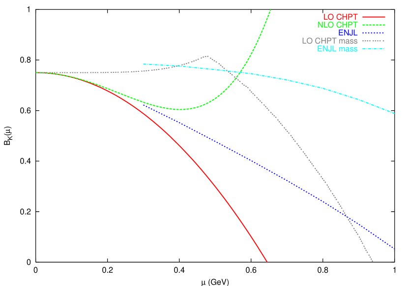
Figure 4: The long-distance part of the $X$-boson exchange calculation. We show $B_{K}(\mu)$ of Eq. (32). The lines are leading- (LO) and next-to-leading-order (NLO) CHPT and the ENJL model for the chiral limit and LO CHPT and the ENJL model for the physical quark masses. Notice the improvement of the ENJL model over CHPT.

We can now put these together with the short distance part with $\alpha_{s}(M_{\tau})=0.334$ and $\mu=\nu$. We use for definiteness the NDR results for $g_{\Delta S=2}$ but we could have used the HV ones with the same answer, see Figure 2. We also included for the massive case the needed correction of $0.09\pm 0.03$ for the octet versus nonet case[8, 12], mainly due to $\eta$-$\eta^{\prime}$ mixing. The result is shown as a function of $\nu$ in Figure 5. Notice the quality of the matching.

In [17] a better identification of the scale together with the Leading-Order CHPT approximation was used, this corresponds to keeping the quadratic divergence only. In the chiral limit this correspond to the first two terms in (35). Negative values for $B_{K}$ and the related 27-plet coupling when using this approximation in the chiral limit (see Figure 5), were also seen there[17]. Notice in the same figure how much the use of higher orders estimated via the ENJL model improves the matching in the chiral limit and outside the chiral limit [12]. The variation is more due to the $\mu$ dependence since as shown in Figure 2 there is little dependence on $\nu$. The massive case has an extremely good stability for 700 MeV to 1 GeV while the chiral case is stable for 550 to 700 MeV.

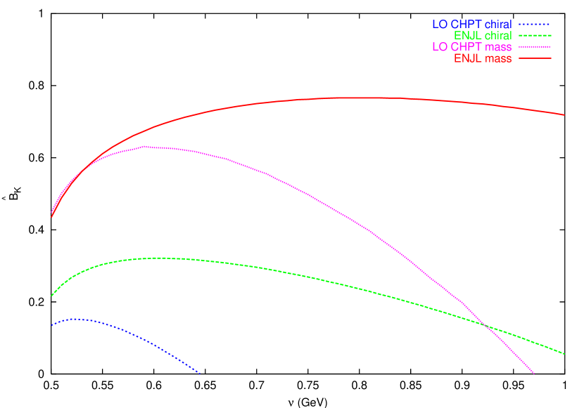
Figure 5: The results for $\hat{B}_{K}$ in the NDR scheme with $\alpha_{s}(M_{\tau})=0.334$ as a function of $\mu=\nu$. The curves are from top to bottom: ENJL massive, leading-order CHPT massive, ENJL chiral limit, leading order CHPT chiral limit. Notice the ENJL stability as compared with leading-order CHPT. Next-to-leading-order CHPT is even more unstable.

As already noted several times before, [8, 12] and references therein, the non-zero quark-mass corrections to $\hat{B}_{K}$ are quite sizable.

We can now study the dependence on the variation with the input. In Figure 6 we have plotted the result with the same input for the HV scheme with the same value for $\alpha_{s}(M_{\tau})$ and in the NDR scheme for $\alpha_{s}(M_{\tau})=0.36$ and $0.31$, including the value of [24]. We took again $\mu=\nu$. The stability is essentially unchanged while the actual values are very similar.

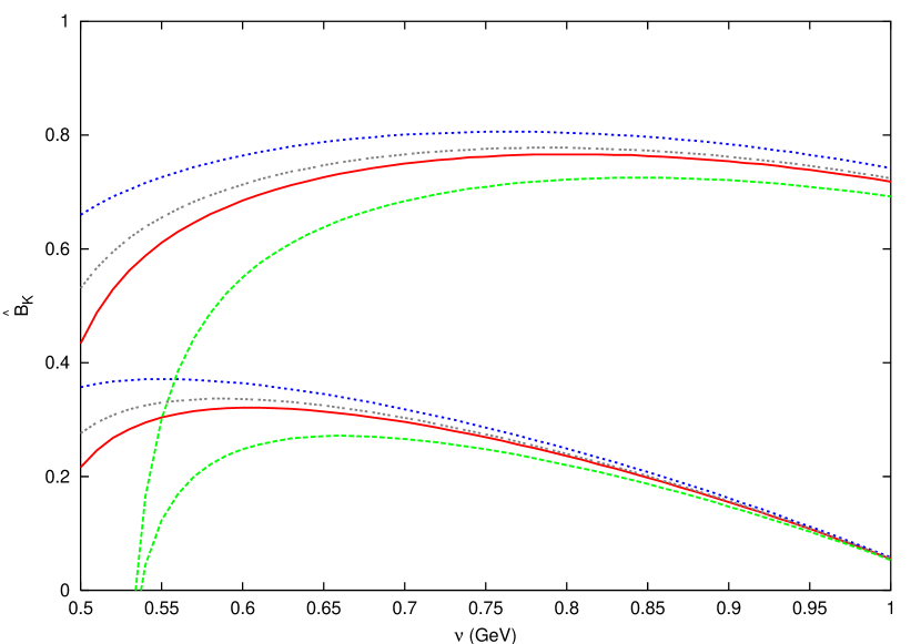
Figure 6: The variation of $\hat{B}_{K}$ with $\alpha_{s}$ as a function of $\nu$. The top set of curves is the massive case, the bottom set is the chiral limit case. Curves are from top to bottom: NDR with $\alpha_{s}(M_{\tau})=0.31$; HV with $\alpha_{s}(M_{\tau})=0.334$; NDR with $\alpha_{s}(M_{\tau})=0.334$; NDR with $\alpha_{s}(M_{\tau})=0.36$.

Finally we want to check the variation with $\mu\neq\nu$. This again provides a check on neglected corrections of order $\alpha_{s}^{2}$. In Figure 7 we plotted the NDR case for $\alpha_{s}(M_{\tau})=0.334$ as a function of $\mu$ for, from top to bottom, $\nu=(1.5,1.2,1,0.8)\mu$. The last curve we did not plot for low values of $\mu$ since this gets very large values for $\alpha_{s}(\nu)$. Again, the variation is rather small.

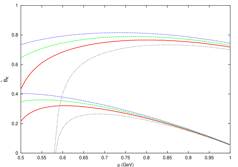
Figure 7: The variation of $\hat{B}_{K}$ in the NDR scheme for, from top to bottom, $\nu=(1.5,1.2,1,0.8)\mu$. The top set of curves shows the massive case, the bottom set the chiral limit.

The uncertainty can be judged from all these variations. We use the variation with $\alpha_{s}(M_{\tau})$ and add a similar error for the remaining model uncertainty to obtain the result given in Eq. (6).

5 Some Remarks on the ENJL Model and Possible Improvements

The model we use has the chiral structure of QCD at large $N_{c}$, i.e. it is a left-right symmetric model which breaks down to the vector subgroup. Quark masses break this symmetry as in QCD.

It provides a picture of build-up of constituent quarks out of massless ones. It has two drawbacks, it doesn’t confine and in some channels it does not reproduce the same high-energy behaviour as QCD. These violations are small at low-energies. It reproduces CHPT to order $p^{4}$ [23], and provides an estimate of all the higher order corrections. It reproduces a large amount of low-energy phenomenology for both the anomalous and the non-anomalous sectors [23] with an accuracy at the level of 20% to 30%.

The drawbacks we think will not affect our numerical results too much because:

1. We do all our integrations in the Euclidean domain. Here the effect of sharp states are smeared out so a model without confinement that reproduces smeared quantities correctly should be all right.

2. We only use the ENJL model at intermediate momenta where CHPT fails and QCD might not work yet. The good matching we obtain is an indication that in the regime where we use it the ENJL model works satisfactorily.

The model works all right but is still the weak link in our approach. Work on some matrix-elements using more direct QCD based arguments has been done[21, 25] and alternatively, we can augment the ENJL model in ways that improve the matching with QCD by requiring matching in as many relevant Green functions as possible.

6 Conclusions

In this paper we have shown how the short-distance large logarithms can be resummed in a consistent fashion while retaining the beauty of the $1/N_{c}$ approach. We have thus shown how to realize Bardeen’s picture of tracking scheme-dependence all the way [4, 5] from the $W$-boson mass to very low scales. The approach is general but we illustrated it in the case of the $B_{K}$ parameter explicitly.

The main assumption is that we know how to hadronize quark currents, once that is done, our approach tells how the four-quark operators should be hadronized. This can be systematically improved by higher order calculations within the perturbative domain. The low-energy hadronic realization of currents of QCD is the only remaining model dependence. At very low energies we know that CHPT describes the QCD behaviour correctly, thus this should be included. In the intermediate domain we can try to use data as much as possible and/or models with various QCD constraints. We have argued that the ENJL model is a good first step beyond CHPT and our final results show this improvement.

By varying $\alpha_{s}$, the matching scales and conditions, i.e. $\mu\neq\nu$ we can get an estimate for the error involved. Our final result for $\hat{B}_{K}$ is:

$$\hat{B}_{K} = 0.77\pm 0.05\;(\alpha_{s})\;\pm 0.05\;(\mbox{model});$$

$$\hat{B}_{K}^{\chi} = 0.32\pm 0.06\;(\alpha_{s})\;\pm 0.12\;(\mbox{model}).$$ (36)

The difference between these results and the ones in [8, 12] is only the short-distance scheme dependence. Our results here are short-distance scheme independent. The main uncertainty are the value of $\alpha_{s}(M_{\tau})$, and a similar error for the remaining model dependence. The small model dependence error we quote is due to the almost cancellation of the $1/N_{c}$ corrections, remember $\hat{B}_{K}=0.75$ at leading order in $1/N_{c}$. Possible systematic errors are of course difficult to estimate. The scale and scheme dependence are consistently matched at order $\alpha_{s}^{2}$ for current $\times$ current operators and are only a small part of the final error, especially for the physically relevant massive case.

The scheme dependence has not been discussed in other non-leptonic weak matrix elements calculations like the $1/N_{c}$ technique in [17] or the chiral quark model in [26].

We will apply the same procedure to the $\Delta S=1$ transitions where first results on the $\Delta I=1/2$ rule were obtained in [12] using $r_{1}^{NDR}$ from [10] and $\tilde{r}_{1}=0$. Work is in progress to perform the remaining calculations also for $\Delta S=1$ transitions and $\varepsilon^{\prime}/\varepsilon$[16].

References

- [1] Proc. of the Workshop on K Physics, Orsay, France, L. Iconomidou-Fayard (ed), Editions Frontières, 1997
- [2] See http://hep.uchicago.edu/kaon99/
- [3] W.A. Bardeen, A.J. Buras, and J.-M. Gérard, Nucl. Phys. B 293 (1987) 787; Phys. Lett. B 192 (1987) 138; Phys. Lett. B 211 (1988) 343; A.J. Buras and J.-M. Gérard, Nucl. Phys. 7A (Proc. Suppl.) (1989) 375; J.-M. Gérard, Acta Phys. Polon. B 21 (1990) 257; A.J. Buras in CP Violation, C. Jarlskog (ed), World Scientific (1989) p. 575
- [4] W.A. Bardeen, Nucl. Phys. 7A (Proc. Suppl.) (1989) 149
- [5] W.A. Bardeen, Weak Matrix Elements in the Large Limit, preprint FERMILAB-Conf-99/255-T, to be published in Proc. of Kaon ’99, Chicago, USA, June 1999
- [6] W.A. Bardeen, J. Bijnens, and J.-M. Gérard, Phys. Rev. Lett. 62 (1989) 1343
- [7] J. Bijnens, G. Klein, and J.-M. Gérard, Phys. Lett. B 257 (1991) 191
- [8] J. Bijnens and J. Prades, Phys. Lett. B 342 (1995) 331; Nucl. Phys. B 444 (1995) 523
- [9] A.J. Buras, Weak Hamiltonian, CP-Violation and Rare Decays, Les Houches lectures, 1998, hep-ph/9806471; G. Buchalla, A.J. Buras, and M. Lautenbacher, Rev. Mod. Phys. 68 (1996) 1125
- [10] G. Altarelli, G. Curci, G. Martinelli, and S. Petrarca, Nucl. Phys. B 187 (1981) 461 A.J. Buras, M. Jamin, M.E. Lautenbacher, and P.H. Weisz, Nucl. Phys. B 370 (1992) 69; addendum ibid. 375 (1992) 501; Nucl. Phys. B 400 (1993) 35; ibid. 400 (1993) 75; A.J. Buras, M. Jamin and M.E. Lautenbacher, Nucl. Phys. B 408 (1993) 209; M. Ciuchini, E. Franco, G. Martinelli, and L. Reina, Nucl. Phys. B 415 (1994) 403; M. Ciuchini, E. Franco, G. Martinelli, L. Reina, and L. Silvestrini, Z. Physik C 68 (1995) 239
- [11] A.J. Buras, M. Jamin, and P.H. Weisz, Nucl. Phys. B 347 (1990) 491; S. Herrlich and U. Nierste, Nucl. Phys. B 419 (1994) 292; Phys. Rev. D 52 (1995) 6505; Nucl. Phys. B 476 (1996) 27; M. Ciuchini, E. Franco, V. Lubicz, G. Martinelli, I. Scimemi, and L. Silvestrini, Nucl. Phys. B 523 (1998) 501
- [12] J. Bijnens and J. Prades, J. High Energy Phys. 01 (1999) 023
- [13] J. Bijnens, hep-ph/9907307; hep-ph/9907514; hep-ph/9910263; hep-ph/9910415; J. Prades, hep-ph/9909245
- [14] G. Altarelli and L. Maiani, Phys. Lett. B 52 (1974) 351; M.K. Gaillard and B.W. Lee, Phys. Rev. Lett. 33 (1974) 108; A.I. Vainshtein, V.I. Zakharov, and M.A. Shifman, Sov. Phys. JETP 45 (1977) 670; F. Gilman and M.B. Wise, Phys. Rev. D 20 (1979) 2392; B. Guberina and R. Peccei, Nucl. Phys. B 163 (1980) 289; J. Bijnens and M.B. Wise, Phys. Lett. B 137 (1984) 245
- [15] M. Ciuchini, E. Franco, L. Giusti, V. Lubicz, and G. Martinelli, hep-ph/9910237
- [16] J. Bijnens, E. Pallante, and J. Prades, work in progress
- [17] T. Hambye and P.H. Soldan, Eur. Phys. J. C 10 (1999) 271; hep-ph/9908232; T. Hambye, G. Köhler, E.A. Paschos, and P.H. Soldan, hep-ph/990634; T. Hambye, G. Köhler, E.A. Paschos, P.H. Soldan, and W.A. Bardeen Phys. Rev. D 58 (1998) 014017
- [18] A.J. Buras and P.H. Weisz, Nucl. Phys. B 333 (1990) 66
- [19] J. Bijnens and J. Prades, Nucl. Phys. B 490 (1997) 239
- [20] J. Bijnens, Phys. Lett. B 306 (1993) 343
- [21] M. Knecht, S. Peris, and E. de Rafael, Phys. Lett. B 443 (1998) 255
- [22] R. Barate et al., ALEPH Coll., Eur. Phys. J. C 4 (1998) 409
- [23] J. Bijnens, C. Bruno, E. de Rafael, Nucl. Phys. B 390 (1993) 501; J. Bijnens, H. Zheng, and E. de Rafael, Z. Physik C 62 (1994) 437; J. Prades, Z. Physik C 63 (1994) 491, Erratum Eur. Phys. J. C, to be published; J. Bijnens and J. Prades, Phys. Lett. B 320 (1994) 130; Z. Physik C 64 (1994) 475; J. Bijnens, Phys. Rept. 265 (1996) 369
- [24] A. Pich, Tau physics in Heavy flavours II, A.J. Buras and M. Lindner (eds.), World Scientific (1998), p. 453, hep-ph/9704453
- [25] S. Peris, M. Perrottet, and E. de Rafael, J. High Energy Phys. 05 (1998) 011; M. Knecht, S. Peris, M. Perrottet, and E. de Rafael, hep-ph/9908283; M. Knecht, S. Peris, and E. de Rafael, hep-ph/9910396
- [26] S. Bertolini, hep-ph/9908268; S. Bertolini, J.O. Eeg, and M. Fabbrichesi, hep-ph/9802405, Nucl. Phys. B 476 (1996) 225; S. Bertolini, J.O. Eeg, M. Fabbrichesi, and E.I. Lashin, Nucl. Phys. B 514 (1998) 63; ibid. 514 (1998) 93; V. Antonelli, S. Bertolini, M. Fabbrichesi, and E.I. Lashin, Nucl. Phys. B 493 (1997) 281, ibid. 469 (1996) 181; V. Antonelli, S. Bertolini, J.O. Eeg, M. Fabbrichesi, and E.I. Lashin, Nucl. Phys. B 469 (1996) 143