Theory of Rare B Meson Decays

Abstract:

I review the NLO QCD calculations of the branching ratio for $B\rightarrow X_{s}\gamma$ in the SM. Including the leading electromagnetic corrections, one obtaines $BR(B\rightarrow X_{s}\gamma)=(3.32\pm 0.30)\times 10^{-4}$. Confronting theory with the newest data, an updated value for $|V_{ts}|$ is obtained: $|V_{ts}|=0.037\pm 0.007$. Theoretical progress on the photon energy spectrum is also discussed. The inclusive FCNC semileptonic decays in the SM are briefly summarized. Furthermore, $B\rightarrow X_{s}\gamma$ is considered in 2HDMs and in different SUSY scenarios. QCD corrections are shown to be crucial.

1 Introduction

In the Standard model (SM), rare $B$ meson decays are induced by one-loop diagrams, where $W$ bosons and up-type quarks are exchanged. In many extensions of the SM, there are additional contributions, where the SM particles in the loop are replaced by nonstandard ones, like charged Higgs bosons, gluinos, charginos etc. Being induced also at the one loop-level, the new physics contributions are not necessarily suppressed relative to the SM one. The resulting sensitivity for nonstandard effects implies the possibility for an indirect observation of new physics, or allows to put limits on the masses and coupling parameters of the new particles. A general overview, where many $B$ physics observables are investigated w.r.t. new physics, was given at this conference by A. Masiero [1]. Concerning the new physics aspects of rare $B$ decays, I concentrate in this article (see sections 3 and 4) on recent calculations of the branching ratio for the process $B\rightarrow X_{s}\gamma$ in a general class of two-Higgs-doublet models (2HMDs) [2, 3] and in supersymmetric scenarios [4, 5, 6], stessing in particular the importance of leading- (LO) and next-to-leading (NLO) QCD corrections.

However, also in the absence of new physics, rare $B$ decays are very important; they can be used for the determination of various CKM matrix elements, occurring in the SM Lagrangian. To extract these parameters from data, it is crucial that the corresponding decay rates are reliably calculable. An important class of such decays are the inclusive rare $B$ decays, like $B\rightarrow X_{s}\gamma$, $B\rightarrow X_{s}\ell^{+}\ell^{-}$, $B\rightarrow X_{s}\nu\bar{\nu}$, $B\rightarrow X_{d}\gamma$, $B\rightarrow X_{d}\ell^{+}\ell^{-}$, $B\rightarrow X_{d}\nu\bar{\nu}$, which are sensitive to the CKM matrix elements $|V_{ts}|$ and $|V_{td}|$, respectively. In contrast to the corresponding exclusive channels, these inclusive decay modes are theoretically cleaner, in the sense that no specific model is needed to describe the final hadronic state. Nonperturbative effects in the inclusive modes are well under control due to heavy quark effective theory. For example, the decay width $\Gamma(B\rightarrow X_{s}\gamma)$ is well approximated by the partonic decay rate $\Gamma(b\rightarrow X_{s}\gamma)$ which can be analyzed in renormalization group improved perturbation theory. The class of non-perturbative effects which scale like $1/m_{b}^{2}$ is expected to be well below $10\%$ [7]. This numerical statement also holds for the non-perturbative contributions which scale like $1/m_{c}^{2}$ [8, 9].

The framework and the NLO theoretical results for the branching ratio of the decay $B\rightarrow X_{s}\gamma$ are discussed in section 2.1; the photon energy spectrum and the partially integrated branching ratio for this process are reviewed in section 2.2; an updated value for the CKM matrix element $|V_{ts}|$, extracted from the most recent measurements of $BR(B\rightarrow X_{s}\gamma)$ and the corresponding calculations, where also the leading electromagnetic corrections are included, is given in section 2.3; the other inclusive rare decays mentioned above, are briefly discussed in section 2.4.

The exclusive analogues, $B\rightarrow K^{*}\gamma$, $B\rightarrow K^{(*)}\ell^{+}\ell^{-}$, $B\rightarrow\rho\gamma$, $B\rightarrow\rho\ell^{+}\ell^{-}$ etc., require the calculation of form factors. As the QCD sum rule calculations and the lattice results for these form factors were summarized by V. Braun [10], I do not discuss these decays in the following.

Finally, there is the class of non-leptonic two-body decays, like $B\rightarrow\pi\pi$, $B\rightarrow K\pi$; the theoretical status of these processes was discussed by L. Silvestrini [11], and new CLEO results were presented by D. Jaffe [12].

2 Inclusive rare $B$ meson decays in the SM

2.1 $BR(B\rightarrow X_{s}\gamma)$ at NLO precision

Short distance QCD effects enhance the partonic decay rate $\Gamma(b\rightarrow s\gamma)$ by more than a factor of two. Analytically, these QCD corrections contain large logarithms of the form $\alpha_{s}^{n}(m_{b})\,\log^{m}(m_{b}/M)$, where $M=m_{t}$ or $M=m_{W}$ and $m\leq n$ (with $n=0,1,2,...$). In order to get a reasonable prediction for the decay rate, it is evident that one has to resum at least the leading-log (LO) series ($m=n$). As the error of the LO result [13] was dominated by a large renormalization scale dependence at the $\pm 25\%$ level, it became clear that even the NLO terms of the form $\alpha_{s}(m_{b})\,\left(\alpha_{s}^{n}(m_{b})\,\ln^{n}(m_{b}/M)\right)$ have to be taken into account systematically.

To achieve the necessary resummations, one usually contructs in a first step an effective low-energy theory and then resums the large logarithms by renomalization group techniques. The low energy theory is obtained by integrating out the heavy particles which in the SM are the top quark and the $W$-boson. The resulting effective Hamiltonian relevant for $b\rightarrow s\gamma$ in the SM and many of its extensions reads

$$H_{eff}^{W}(b\rightarrow s\gamma)=-\frac{4G_{F}}{\sqrt{2}}\,\lambda_{t}\,\sum_{i=1}^{8}C_{i}(\mu)\,O_{i}(\mu)\quad,$$ (1)

where $O_{i}(\mu)$ are local operators consisting of light fields, $C_{i}(\mu)$ are the corresponding Wilson coefficients, which contain the complete top- and $W$- mass dependence, and $\lambda_{t}=V_{tb}V_{ts}^{*}$ with $V_{ij}$ being the CKM matrix elements. The CKM dependence globally factorizes, because we work in the approximation $\lambda_{u}=0$.

Retaining only operators up to dimension 6 and using the equations of motion, one arrives at the following basis

$$O_{1} = \left(\bar{c}_{L\beta}\gamma^{\mu}b_{L\alpha}\right)\,\left(\bar{s}_{L\alpha}\gamma_{\mu}c_{L\beta}\right)\,,$$

$$O_{2} = \left(\bar{c}_{L\alpha}\gamma^{\mu}b_{L\alpha}\right)\,\left(\bar{s}_{L\beta}\gamma_{\mu}c_{L\beta}\right)\,,$$

$$O_{7} = \frac{e}{16\pi^{2}}\,\bar{s}_{\alpha}\,\sigma^{\mu\nu}\,(m_{b}(\mu)R)\,b_{\alpha}\ F_{\mu\nu}\,,$$

$$O_{8} = \frac{g_{s}}{16\pi^{2}}\,\bar{s}_{\alpha}\,\sigma^{\mu\nu}\,(m_{b}(\mu)R)\,\frac{\lambda^{A}_{\alpha\beta}}{2}\,b_{\beta}\ G^{A}_{\mu\nu}\quad.$$ (2)

As the Wilson coefficients of the QCD penguin operators $O_{3},...,O_{6}$ are small, we do not list them here.

It is by now well known that a consistent calculation for $b\rightarrow s\gamma$ at LO (or NLO) precision requires three steps:

• a matching calculation of the full standard model theory with the effective theory at the scale $\mu=\mu_{W}$ to order $\alpha_{s}^{0}$ (or $\alpha_{s}^{1}$) for the Wilson coefficients, where $\mu_{W}$ denotes a scale of order $M_{W}$ or $m_{t}$;

• a renormalization group evolution of the Wilson coefficients from the matching scale $\mu_{W}$ down to the low scale $\mu_{b}=O(m_{b})$, using the anomalous-dimension matrix to order $\alpha_{s}^{1}$ (or $\alpha_{s}^{2}$);

• a calculation of the matrix elements of the operators at the scale $\mu=\mu_{b}$ to order $\alpha_{s}^{0}$ (or $\alpha_{s}^{1}$).

At NLO precision, all three steps are rather involved: The most difficult part in Step 1 is the order $\alpha_{s}$ matching of the dipole operators $O_{7}$ and $O_{8}$. Two-loop diagrams, both in the full- and in the effective theory have to be worked out. This matching calculation was first performed by Adel and Yao [14] and then confirmed by Greub and Hurth [15], using a different method. Later, two further recalculations of this result were presented [3, 16]. The order $\alpha_{s}^{2}$ anomalous matrix (Step 2) has been worked out by Chetyrkin, Misiak and Münz [17]. The extraction of certain elements in this matrix involves the calculation of pole parts of three loop diagrams. Step 3 consists of Bremsstrahlung contributions and virtual corrections. The Brems- strahlung corrections were worked out some time ago by Ali and Greub [18] and have been confirmed and extended by Pott [19]. An analysis of the virtual two loop corrections was presented by Greub, Hurth and Wyler [20].

Combining the NLO calculations of these 3 steps, leads to the following NLO QCD prediction for the branching ratio [2]:

$$BR(B\rightarrow X_{s}\gamma)=\left(3.57\pm^{\,0.01}_{\,0.12}\pm^{\,0.00}_{\,0.08}\pm^{\,0.29}_{\,0.27}\right)\times 10^{-4}\,.$$ (3)

The central value is obtained for $\mu_{b}=4.8\,$GeV, $\mu_{W}=m_{W}$ and the central values of the input parameters listed in [2]. The first error is obtained by varying $\mu_{b}$ in the interval $[2.4,9.6]\,$GeV, the second one by varying the matching scale $\mu_{W}$ between $m_{W}$ and $m_{t}$; the third error reflects the uncertainties in the various input parameters. Similar results were also obtained in refs. [3, 16].

We should mention that in the result (3) also power corrections are included: there are $1/m_{b}^{2}$ corrections [7], whose impact on $BR(B\rightarrow X_{s}\gamma)$ is at the $1\%$ level, as well as nonperturbative contributions from $c\bar{c}$ intermediate states which scale with $1/m_{c}^{2}$. Detailed investigations [8, 9] show that these $1/m_{c}^{2}$ corrections enlarge the branching ratio by $\sim 3\%$.

After the QCD analyses, several papers appeared where different classes of electroweak corrections [21, 22, 23, 24] to $BR(B\rightarrow X_{s}\gamma)$ were considered. In [23], corrections to the Wilson coefficients at the matching scale due to the top quark and the neutral Higgs boson were calculated and found to be negligible. The analysis  [21] concluded that the most appropriate value of $\alpha_{em}^{-1}$ to be used for this problem is the fine structure constant $\alpha^{-1}=137.036$ instead of the value $\alpha_{em}^{-1}=130.3\pm 2.3$ previously used. In [22, 24], the leading logarithmic QED corrections of the form $\alpha\log({\mu_{W}}/{\mu_{b}})\left(\alpha_{s}\log({\mu_{W}}/{\mu_{b}})\right)^{n}$ (with resummation in $n$) were given.

In ref. [25] we updated the result in eq. (3), by including the class of QED corrections presented in [22]; we then obtained

$$BR(B\rightarrow X_{s}\gamma)=\left(3.32\pm^{\,0.00}_{\,0.11}\pm^{\,0.00}_{\,0.08}\pm^{\,0.26}_{\,0.25}\right)\times 10^{-4}\,.$$ (4)

The bulk of the change with respect to the value in eq. (3) is due to the different value of $\alpha_{em}^{-1}$ used.

A remark concerning the error due to the variation of the low scale $\mu_{b}$ in the results (3) and (4) is in order here: As it will be discussed in more detail in section 3, it was realized in [2] that in multi Higgs doublet models the QCD corrections in certain regions of the parameter space are much larger than in the SM. As a consequence, the dependence on the scale $\mu_{b}$ of $BR(B\rightarrow X_{s}\gamma)$ is also larger. Later, Kagan and Neubert pointed out very explicitly in their analysis [22] that the scale dependences in individual contributions to the branching ratio in the SM are larger than their combined effect, due to accidental cancellations. They suggest that one should add the scale uncertainties from the individual contributions in quadrature, in order to get a more reliable estimate of the truncation error. Their estimate for the $\mu_{b}$ dependence of $BR(B\rightarrow X_{s}\gamma)$ is $\pm 6.3\%$, i.e., more than twice the naive estimate. The total error in (4), however, is dominated by parametric uncertainties and therefore gets increased only marginally when using this more conservative estimate of the scale uncertainties.

The measurement of $BR(B\rightarrow X_{s}\gamma)$ by the ALEPH collaboration at LEP [26]

$$BR(B\rightarrow X_{s}\gamma)=(3.11\pm 0.80\pm 0.72)\times 10^{-4}$$ (5)

and by the CLEO collaboration at CESR [27]

$$BR(B\rightarrow X_{s}\gamma)=(3.15\pm 0.35\pm 0.32\pm 0.26)\times 10^{-4}$$ (6)

are in good agreement with the NLO calculation (4), where the most important electromagnetic corrections are included.

2.2 Partially integrated branching ratio in $B\rightarrow X_{s}\gamma$

The photon energy spectrum of the partonic decay $b\rightarrow s\gamma$ is a delta function, concentrated at $\sim(m_{b}/2)$, when the b-quark decays at rest. This delta function gets smeared when considering the inclusive photon energy spectrum from a $B$ meson decay. There is a perturbative contribution to this smearing, induced by the Bremsstrahlung process $b\rightarrow s\gamma g$ [18, 19], as well as a non perturbative one, which is due to the Fermi motion of the decaying $b$ quark in the $B$ meson.

For small photon energies, the $\gamma$-spectrum from $B\rightarrow X_{s}\gamma$ is completely overshadowed by background processes, like $b\rightarrow c\bar{u}d\gamma$ and $b\rightarrow u\bar{u}d\gamma$. This background falls off very rapidly with increasing photon energy, and becomes small for $E_{\gamma}>\sim 2$ GeV [28]. This implies that only the partial branching ratio

$$BR(B\rightarrow X_{s}\gamma)(E_{\gamma}^{min})=\int_{E_{\gamma}^{min}}^{E_{\gamma}^{max}}\frac{dBR}{dE_{\gamma}}dE_{\gamma}$$ (7)

can be directly measured, with $E_{\gamma}^{min}=O(2)$ GeV. Recently, CLEO was able to reduce $E_{\gamma}^{min}$ from 2.2 GeV to 2.1 GeV [27]. To determine from such a measurement the full branching ratio for $B\rightarrow X_{s}\gamma$, one has to know from theory the fraction $R$ of the $B\rightarrow X_{s}\gamma$ events with photon energies above $E_{\gamma}^{min}$. Based on calculations by Ali and Greub [18] of the photon energy spectrum within the Fermi motion model by Altarelli et al. [29], CLEO used the value $R=85\%-94\%$ [27] in order to determine $BR(B\rightarrow X_{s}\gamma)$ from the measured partial branching ratio.

A modern way - based on first principles - implements the Fermi motion in the framework of the heavy-quark expansion. When probing the spectrum closer to the endpoint, the OPE breaks down, and the leading twist non-perturbative corrections must be resummed into the $B$ meson structure function $f(k_{+})$ [30], where $k_{+}$ is the light-cone momentum of the $b$ quark in the $B$ meson. The physical spectrum is then obtained by the convolution

$$\frac{d\Gamma}{dE_{\gamma}}=\int_{2E_{\gamma}-m_{b}}^{\bar{\Lambda}}dk_{+}f(k_{+})\frac{d\Gamma_{part}}{dE_{\gamma}}(m_{b}^{*})\quad,$$ (8)

where $(d\Gamma_{part}/dE_{\gamma})(m_{b}^{*})$ is the partonic differential rate, written as a function of the “effective mass” $m_{b}^{*}=m_{b}+k_{+}$. The function $f(k_{+})$ has support in the range $-\infty<k_{+}<\bar{\Lambda}$, where $\bar{\Lambda}=m_{B}-m_{b}$ in the infinite mass limit. This implies that the addition of the structure function moves the partonic endpoint of the spectrum from $m_{b}/2$ to the physical endpoint $m_{B}/2$. While the shape of the function $f(k_{+})$ is unknown, the first few moments $A_{n}=\int dk_{+}\,k_{+}^{n}f(k_{+})$ are known: $A_{0}=1$, $A_{1}=0$ and $A_{2}=-\lambda_{1}/3$. The values of $\bar{\Lambda}$ and $\lambda_{1}$ are not calculable analytically and have to be extraced from experiments or calculated on the lattice. A recent analysis gives $(\bar{\Lambda},\lambda_{1})=(0.39\pm 0.11\mbox{GeV},-0.19\mp 0.10\mbox{GeV}^{2})$ [31]. As $A_{n}$ ($n>2$) are poorly known, several Ansätze were used for $f(k_{+})$; e.g. Neubert and Kagan [22] used $f(k_{+})=N(1-x)^{a}e^{(1+a)x}$, with $x=k_{+}/\bar{\Lambda}$. Taking into account the constraints from $A_{0}$, $A_{1}$ and $A_{2}$, the independent parameters in this Ansatz can be chosen to be $m_{b}$ and $\lambda_{1}$. As shown in [22], the uncertainty of $m_{b}$ dominates the error of the partial branching ratio.

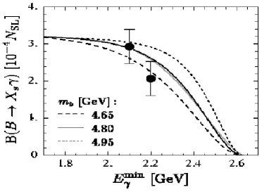
Figure 1: Partially integrated branching ratio as a function of the energy cutoff $E_{\gamma}^{min}$; Figure taken from Neubert and Kagan [22].

In Fig. 1 the partial branching ratio is shown for the relevant range of $m_{b}$ as a function of $E_{\gamma}^{min}$, keeping $\lambda_{1}/\bar{\Lambda}^{2}$ fixed. For comparison, the data point $BR(B\rightarrow X_{s}\gamma)=(2.04\pm 0.47)\times 10^{-4}$, obtained in the original CLEO analysis with a cutoff at 2.2 GeV [32], as well as the new data point $BR(B\rightarrow X_{s}\gamma)=(2.97\pm 0.33\pm 0.30\pm 0.21)\times 10^{-4}$, corresponing to a cutoff at 2.1 GeV [27], are also shown in Fig. 1. We would like to stress that it would be very welcome, if the cutoff could be pushed down to 2.0 GeV, because the theoretical uncertainity drastically becomes smaller, as seen in Fig. 1.

We should add that in the endpoint region also the perturbative contributions, mentioned at the beginning of this section, could become problematic in principle, due to the presence of threshold logs, $\log(1-2E_{\gamma}/m_{b})$. These logarithms have recently been resummed up to next-to-leading logarithmic precision [33]. The authors of this paper conclude that for the present energy cut at 2.1 GeV, these threshold logs do not form a dominant sub-series and therefore their resummation is not necessary for predicting the decay rate. Recently, also the BLM type corrections of the order $\alpha_{s}^{2}\beta_{0}$ to the photon energy spectrum were calculated [34]. The result was used to extract a value for $\bar{\Lambda}$ from the average $\langle 1-2E_{\gamma}/m_{B}\rangle$, and a value for $\lambda_{1}$ from $\langle(1-2E_{\gamma}/m_{B})^{2}\rangle$. According to this analysis, the CLEO data in the region $E_{\gamma}>2.1$ GeV implies the central value $\bar{\Lambda}_{\alpha_{s}}\simeq 390$ MeV and $\bar{\Lambda}_{\alpha_{s}^{2}\beta_{0}}\simeq 270$ MeV at order $\alpha_{s}$ and $\alpha_{s}^{2}\beta_{0}$, respectively. This anlysis was somewhat critisized in ref. [33], by pointing out that other $\alpha_{s}^{2}$ terms could be larger than the BLM terms.

2.3 $|V_{ts}|$ form $B\rightarrow X_{s}\gamma$

Instead of making a prediction for $BR(B\rightarrow X_{s}\gamma)$, one can use the NLO calculation to extract the CKM combination $|V_{tb}V_{ts}^{*}|/|V_{cb}|$ from the measurements; in turn, one can determine $|V_{ts}|$, by making use of the relatively well known CKM matrix elements $V_{cb}$ and $V_{tb}$. Using the CLEO (6) and ALEPH data (5), one obtains [35]

$$\frac{|V_{ts}^{*}V_{tb}|}{|V_{cb}|}=0.93\pm 0.09_{exp.}\pm 0.03_{th}\,.$$ (9)

Using $|V_{tb}|=0.99\pm 0.15$ from the CDF measurement and $|V_{cb}|=0.0393\pm 0.0028$ extracted from semileptonic $B$ decays, one obtains

$$|V_{ts}|=0.037\pm 0.007,$$ (10)

where all the errors were added in quadrature. This is probably the most direct determination of this CKM matrix element, as the measurement of $t\rightarrow sW^{+}$ seems to be difficult. With an improved measurement of $BR(B\rightarrow X_{s}\gamma)$ and $V_{tb}$, one expects to reduce the present error on $|V_{ts}|$ by a factor of 2 or even more.

2.4 $B\rightarrow X_{d}\gamma$, $B\rightarrow(X_{s},X_{d})\ell^{+}\ell^{-}$ and $B\rightarrow(X_{s},X_{d})\nu\bar{\nu}$ in the SM

The decay $B\rightarrow X_{d}\gamma$ can be treated in a similar way as $B\rightarrow X_{s}\gamma$ [36]. The only difference is that $\lambda_{u}$ for $b\rightarrow d\gamma$ is not small relative to $\lambda_{t}$ and $\lambda_{c}$; therefore, also the current-current operators $O_{1}^{u}$ and $O_{2}^{u}$, weighted by $\lambda_{u}$, contribute. Unfortunately, these operators induce long-distance contributions to $B\rightarrow X_{d}\gamma$, which at present only can be estimated using models. In ref. [36], these long-distance effects were absorbed into the theoretical error.

Using $\mu_{b}=2.5$ GeV and the central values of the input parameters, the analysis in ref. [36] yields a difference between the LO and NLO predictions for $BR(B\rightarrow X_{d}\gamma)$ of $\sim 10\%$, increasing the branching ratio in the NLO case. For a fixed value of the CKM-Wolfenstein parameters $\rho$ and $\eta$, the theoretical uncertainty of the average branching ratio $\langle BR(B\rightarrow X_{d}\gamma)\rangle$ of the decay $B\rightarrow X_{d}\gamma$ and its charge conjugate $\overline{B}\rightarrow\overline{X_{d}}\gamma$ is: $\Delta\langle BR(B\rightarrow X_{d}\gamma)\rangle/\langle BR(B\rightarrow X_{d}\gamma)\rangle=\pm(6-10)\%$. Of particular theoretical interest for constraining $\rho$ and $\eta$ is the ratio of the branching ratios, defined as

$$R(d\gamma/s\gamma)\equiv\frac{\langle BR(B\rightarrow X_{d}\gamma)\rangle}{\langle BR(B\rightarrow X_{s}\gamma)\rangle},$$ (11)

in which a good part of the theoretical uncertainties cancels. Varying the CKM-Wolfenstein parameters $\rho$ and $\eta$ in the range $-0.1\leq\rho\leq 0.4$ and $0.2\leq\eta\leq 0.46$ and taking into account other parametric dependences, the results (without electroweak corrections) are

$$6.0\times 10^{-6} \leq BR(B\rightarrow X_{d}\gamma)\leq 2.6\times 10^{-5}~{},$$

$$0.017 \leq R(d\gamma/s\gamma)\leq 0.074~{}.$$

Another observable, which is also sensitive to the CKM parameters $\rho$ and $\eta$, is the CP rate asymmetry $a_{CP}$, defined as

$$a_{CP}=\frac{\Gamma(B\rightarrow X_{d}\gamma)-\Gamma(\overline{B}\rightarrow\overline{X_{d}}\gamma)}{\Gamma(B\rightarrow X_{d}\gamma)+\Gamma(\overline{B}\rightarrow\overline{X_{d}}\gamma)}\,.$$ (12)

Varying $\rho$ and $\eta$ in the range specified above, we obtained $7\%\leq a_{CP}\leq 35\%$ [36]. We would like to point out that $a_{CP}$ is at the moment only available to LO precision and therefore suffers from a relatively large renormalization scale dependence.

A measurement of the semileptonic FCNC decays $B\rightarrow X_{s}\ell^{+}\ell^{-}$ and $B\rightarrow X_{d}\ell^{+}\ell^{-}$, below the $J/\psi$- and above the $\rho,\omega$-resonance regions in the dilepton invariant mass, can also be used to extract $|V_{ts}|$ and $|V_{td}|$, respectively. In this context, these decays and the related ones, $B\rightarrow X_{s}\nu\bar{\nu}$ and $B\rightarrow X_{d}\nu\bar{\nu}$, were discussed some time ago [37]. The decays $B\rightarrow(X_{s},X_{d})\nu\bar{\nu}$ are practically free of long-distance contributions [9] and the renormalization scale dependence of these decay rates has also been brought under control [38]. Hence, these decays are theoretically remarkably clean but, unfortunately, they are difficult to measure. The ALEPH collaboration has searched for the decay $B\rightarrow X_{s}\nu\bar{\nu}$, setting an upper bound $BR(B\rightarrow X_{s}\nu\bar{\nu})<7.7\times 10^{-4}$ (at 90% C.L.) [39], which is a factor 20 away from the SM expectations [38].

In contrast, the prediction of the decay rate $\Gamma(B\rightarrow X_{s}\ell^{+}\ell^{-})$ still suffers from many uncertainties. The most important ones are due to intermediate $c\bar{c}$ states. Because of the non perturbative nature of these states, the differential spectrum can be only roughly estimated when the invariant mass $m_{\ell^{+}\ell^{-}}$ is not sufficiently below $m_{J/\psi}$. However, for low $\hat{s}=m_{\ell^{+}\ell^{-}}^{2}/m_{b}^{2}$, a relatively precise determination of the spectrum is possible using perturbative methods only, up to calculable HQET corrections. The dominant HQET corrections were evaluated and found to be smaller than 6% for $0.05<\hat{s}<0.25$. Therefore, the $B\rightarrow X_{s}\ell^{-}\ell^{+}$ rate integrated over this region of $\hat{s}$ should be perturbatively predictable as precisely as $\Gamma(B\rightarrow X_{s}\gamma)$, i.e. up to about 10% uncertainty. However, the presently available NLO QCD corrections [40, 41] have not yet reached this precision. The formally LO term is suppressed, which makes it as small as some of the NLO contributions. Consequently, some NNLO terms still can be large. The NNLO program for this decay was recently started [43], by calculating the two-loop matching conditions for all the operators relevant for $B\rightarrow X_{s}\ell^{+}\ell^{-}$. The improved matching allows to remove an important ($\sim\pm 16\%$) matching scale uncertainty for $BR(B\rightarrow X_{s}\ell^{+}\ell^{-})$ in the mentioned region of $\hat{s}$, leading to $BR(B\rightarrow X_{s}\ell^{+}\ell^{-})=1.46\times 10^{-6}$. A remaining perturbative uncertainty of about 13%, due to the unknown two-loop matrix elements of the four-quark operators, was also estimated in ref. [43].

3 $B\rightarrow X_{s}\gamma$ in generalized two-Higgs Doublet models

Two Higgs Doublet Models (2HDMs) are conceptually among the simplest extensions of the SM. Studies of $BR(B\rightarrow X_{s}\gamma)$ in these models can already test whether the observed high accuracy of the NLO SM result is a generic feature of NLO calculations [2, 25] or a rather particluar one, valid for the SM only. Such studies can obviously provide also important indirect bounds on the new parameters contained in these models.

The well–known Type I and Type II models are particular examples of 2HDMs, in which the same or the two different Higgs fields couple to up– and down–type quarks. The second one is especially important since it has the same couplings of the charged Higgs $H^{+}$ to fermions that are present in the Minimal Supersymmetric Standard Model (MSSM). The couplings of the neutral Higgs to fermions have important differences from those of the MSSM [44, 45]. However, since beside the $W$, only charged Higgs bosons mediate the decay $B\rightarrow X_{s}\gamma$ when additional Higgs doublets are present, the predictions of $BR(B\rightarrow X_{s}\gamma)$ in a 2HDM of Type II give, at times, a good approximation of the value of this branching ratio in some supersymmetric models [46].

It is implicit in our previous statements that we do not consider scenarios with tree–level flavour changing couplings to neutral Higgs bosons. We do, however, generalize our class of models to accommodate Multi–Higgs Doublet models, provided only one charged Higgs boson remains light enough to be relevant for the process $B\rightarrow X_{s}\gamma$. This generalization allows a simultaneous study of different models, including Type I and Type II, by a continuous variation of the (generally complex) charged Higgs couplings to fermions. It allows also a more complete investigation of the question whether the measurement of $BR(B\rightarrow X_{s}\gamma)$ closes the possibility of a relatively light $H^{\pm}$ not embedded in a supersymmetric model.

We will show that the NLO QCD corrections to the Higgs contributions to $BR(B\rightarrow X_{s}\gamma)$ are much larger than the corresponding corrections to the SM contribution [2], irrespectively of the value of the charged Higgs couplings to fermions. This feature remains undetected in Type II models, where the SM contribution to $BR(B\rightarrow X_{s}\gamma)$ is always larger than, and in phase with, the Higgs contributions. In this case, a comparison between theoretical and experimental results for $BR(B\rightarrow X_{s}\gamma)$ allows to conclude that values of $m_{H^{\pm}}=O(m_{W})$ can be excluded. Such values are, however, still allowed in other 2HDMs.

These issues are illustrated in Sec. 3.3, after defining in Sec. 3.1 the class of 2HDMs considered, and presenting the NLO corrections at the amplitude level in Sec. 3.2.

3.1 Couplings of Higgs bosons to fermions

Models with $n$ Higgs doublets have generically a Yukawa Lagrangian (for the quarks) of the form:

$$-h^{d}_{ij}\,{\overline{q^{\prime}}_{L}}_{i}\,\phi_{1}\,{d^{\prime}_{R}}_{j}-h^{u}_{ij}\,{\overline{q^{\prime}}_{L}}_{i}\,{\widetilde{\phi}}_{2}\,{u^{\prime}_{R}}_{j}+{\rm h.c.}\,,$$ (13)

where $q^{\prime}_{L}$, $\phi_{i}$, ($i=1,2$) are SU(2) doublets (${\widetilde{\phi}_{i}}=i\sigma^{2}\phi_{i}^{*}$); $u^{\prime}_{R}$, $d^{\prime}_{R}$ are SU(2) singlets and $h^{d}$, $h^{u}$ denote $3\times 3$ Yukawa matrices. To avoid flavour changing neutral couplings at the tree–level, it is sufficient to impose that no more than one Higgs doublet couples to the same right–handed field, as in eq. (13).

After a rotation of the quark fields from the current eigenstate to the mass eigenstate basis, and an analogous rotation of the charged Higgs fields through a unitary $n\times n$ matrix $U$, we assume that only one of the $n-1$ charged physical Higgs bosons is light enough to lead to observable effects in low energy processes. The $n$–Higgs doublet model then reduces to a generalized 2HDM, with the following Yukawa interaction for this charged physical Higgs boson denoted by $H^{+}$:

$$\frac{g}{\sqrt{2}}\left\{X\,{\overline{u}_{L}}V\frac{m_{d}}{m_{W}}\,{d_{R}}+Y\,{\overline{u}_{R}}\frac{m_{u}}{m_{W}}V\,d_{L}\right\}H^{+}$$ (14)

In (14), $V$ is the Cabibbo–Kobayashi–Maskawa matrix and the symbols $X$ and $Y$ are defined in terms of elements of the matrix $U$ (see citations in ref. [2]). Notice that $X$ and $Y$ are in general complex numbers and therefore potential sources of CP violating effects. The ordinary Type I and Type II 2HDMs (with $n=2$), are special cases of this generalized class, with $(X,Y)=(-\cot\beta,\cot\beta)$ and $(X,Y)=(\tan\beta,\cot\beta)$, respectively.

3.2 NLO corrections at the amplitude level

It turns out that the charged Higgs contributions do not induce operators in addition to those in the SM Hamiltonian $H_{eff}^{W}$ in eq. (1). More specifically, only step 1) below eq. (2.1), gets modified when adding the charged Higgs boson contributions to the SM one. The new contributions to the matching conditions have been worked out independently by several groups [47, 3, 2], by simultaneously integrating out all heavy particles, $W$, $t$, and $H^{+}$ at the scale $\mu_{W}$. This is a reasonable approximation provided $m_{H^{\pm}}$ is of the same order of magnitude as $m_{W}$ or $m_{t}$.

Indeed, the lower limit on $m_{H^{\pm}}$ coming from LEP I, of $45\,$GeV, guarantees already $m_{H^{\pm}}=O(m_{W})$. There exists a higher lower bound from LEP II of $55\,$GeV for any value of $\tan\beta$ [48] for Type I and Type II models, which has been recently criticized in ref. [45]. This criticism is based on the fact that there is no lower bound on $m_{A}$ and/or $m_{H}$ coming from LEP [44, 49].

After performing steps 1), 2), and 3) listed below eq. (2.1), it is easy to obtain the quark level amplitude $A(b\rightarrow s\gamma)$. As the matrix elements $\langle s\gamma|O_{i}|b\rangle$ are proportional to the tree–level matrix element of the operator $O_{7}$, the amplitude $A$ can be written in the compact form

$$A(b\rightarrow s\gamma)=\frac{4G_{F}}{\sqrt{2}}V_{tb}V_{ts}^{*}\,\overline{D}\,\langle s\gamma|O_{7}|b\rangle_{tree}\quad.$$ (15)

For the following discussion it is useful to decompose the reduced amplitude $\overline{D}$ in such a way that the dependence on the couplings $X$ and $Y$ (see eq. (14)) becomes manifest:

$$\overline{D}=\overline{D}_{\rm SM}+XY^{*}\overline{D}_{\rm XY}+|Y|^{2}\overline{D}_{\rm YY}\quad.$$ (16)

Figure 2: LO (dashed) and NLO (solid) predictions of the various pieces of the reduced amplitude $\overline{D}$ for $m_{H^{\pm}}=100\,$GeV (see text).

In Fig. 2 the individual $\overline{D}$ quantities are shown in LO (dashed) and NLO (solid) order, for $m_{H^{\pm}}=100$ GeV, as a function of $\mu_{b}$; all the other input parameters are taken at their central values, as specified in ref. [2]. To explain the situation, one can concentrate on the curves for $\overline{D}_{\rm XY}$. Starting from the LO curve (dashed), the final NLO prediction is due to the change of the Wilson coefficient $C_{7}$, shown by the dotted curve, and by the inclusion of the virtual QCD corrections to the matrix elements. This results into a further shift from the dotted curve to the solid curve. Both effects contribute with the same sign and with similar magnitude, as it can be seen in Fig. 2. The size of the NLO corrections in the term $\overline{D}_{\rm XY}$ in (16) is

$$\frac{\Delta\overline{D}_{\rm XY}}{\overline{D}_{\rm XY}^{LO}}\equiv\frac{\overline{D}_{\rm XY}^{NLO}-\overline{D}_{\rm XY}^{LO}}{\overline{D}_{\rm XY}^{LO}}\sim-40\%\,!$$ (17)

A similarly large correction is also obtained for $\overline{D}_{\rm YY}$. For the SM contribution $\overline{D}_{\rm SM}$, the situation is different: the corrections to the Wilson coefficient $C_{7}$ and the corrections due to the virtual corrections in the matrix elements are smaller individually, and furthermore tend to cancel when combined, as shown in Fig. 2

The size of the corrections in $\overline{D}$ strongly depends on the couplings $X$ and $Y$ (see eq. (16)): $\Delta\overline{D}/\overline{D}$ is small, if the SM dominates, but it can reach values such as $-50\%$ or even worse, if the SM and the charged Higgs contributions are similar in size but opposite in sign.

3.3 Results

The branching ratio $BR(B\rightarrow X_{s}\gamma)$ can be sche- matically written as

$$BR(B\rightarrow X_{s}\gamma)\propto|\overline{D}|^{2}+\cdots\quad,$$ (18)

where the ellipses stand for Bremsstrahlung contributions, electroweak corrections and nonperturbative effects. As required by perturbation theory, $|\overline{D}|^{2}$ in eq. (18) should be understood as

$$|\overline{D}|^{2}=|\overline{D}^{LO}|^{2}\left[1+2\mbox{Re}\left(\frac{\Delta\overline{D}}{\overline{D}^{LO}}\right)\right]\quad,$$ (19)

i.e., the term $|\Delta\overline{D}/\overline{D}^{LO}|^{2}$ is omitted. If $\mbox{Re}(\Delta\overline{D}/$ $\overline{D}^{LO})$ is larger than $50\%$ in magnitude and negative, the NLO branching ratio becomes negative, i.e. the truncation of the perturbative series at the NLO level is not adequate for the corresponding couplings $X$ and $Y$. As shown in ref. [2], this can happen even for modest values of $X$ and $Y$.

However, theoretical predictions for the branching ratio in Type II models stand, in general, on a rather solid ground. Fig. 3 shows the low–scale dependence of $BR(B\rightarrow X_{s}\gamma)$ for matching scale $\mu_{W}=m_{H^{\pm}}$, for $m_{H^{\pm}}>100\,$GeV. It is less than $\pm 10\%$ for any value of $m_{H^{\pm}}$ above the LEP I lower bound of $45\,$GeV.

Figure 3: $BR(B\rightarrow X_{s}\gamma)$ in a Type II model with $\tan\beta=2$, for various values of $\mu_{b}$. The leading QED corrections are included (see text).

Such a small scale uncertainty is a generic feature of Type II models and remains true for values of $\tan\beta$ as small as $0.5$. In this, as in the following figures where reliable NLO predictions are presented, the recently calculated leading QED corrections are included in the way discussed in the addendum [25] of ref. [2]. They are not contained in the result shown in Fig. 2, which has an illustrative aim only.

In Type II models, the theoretical estimate of $BR(B\rightarrow X_{s}\gamma)$ can be well above the experimental upper bound of $4.5\times 10^{-4}$ ( $95\%$ C.L.) [27], leading to constraints in the $(\tan\beta,m_{H^{\pm}})$ plane. The region excluded by the CLEO bound, as well as by other hypothetical experimental bounds, is given in Fig. 4.

Figure 4: Contour plot in $(\tan\beta,m_{H^{\pm}})$ in Type II models, obtained by using the NLO expression for $BR(B\rightarrow X_{s}\gamma)$ and possible experimental upper bounds. The leading QED corrections are included. The allowed region is above the corresponding curves.

For $\tan\beta=0.5$,1,5, we exclude respectively $m_{H^{\pm}}\leq 280$, 200, 170 GeV, using the present upper bound from CLEO.

Also in the case of complex couplings, the results for $BR(B\rightarrow X_{s}\gamma)$ range from ill–defined, to uncertain, up to reliable. One particularly interesting case in which the perturbative expansion can be safely truncated at the NLO level, is identified by: $Y=1/2$, $X=2\exp(i\phi)$, and $m_{H^{\pm}}=100\,$GeV. The corresponding branching ratios, shown in Fig. 5, are consistent with the CLEO measurement, even for a relatively small value of $m_{H^{\pm}}$ in a large range of $\phi$. Such a light charged Higgs can contribute to the decays of the $t$–quark, through the mode $t\rightarrow H^{+}b$.

Figure 5: $BR(B\rightarrow X_{s}\gamma)$ as a function of $\phi$, where $\phi$ parametrizes $X=2\exp(i\phi)$, for $Y=1/2$, $m_{H^{\pm}}=100$ GeV. Solid, dashed and dash–dotted lines correspond to $\mu_{b}=4.8,2.4,9.6$ GeV. The leading QED corrections are included (see text). Superimposed is the range of values allowed by the CLEO measurement.

The imaginary parts in the $X$ and $Y$ couplings induce –together with the absorptive parts of the NLO loop-functions– CP rate asymmetries in $B\rightarrow X_{s}\gamma$. A priori, these can be expected to be large. We find, however, that choices of the couplings $X$ and $Y$ which render the branching ratio stable, induce in general small asymmetries, not much larger than the modest value of $1\%$ obtained in the SM [36].

4 $B\rightarrow X_{s}\gamma$ in SUSY models

Rare decays also provide guidelines for supersymmetry model building. Their observation, or the upper limits set on them, yields stringent constraints on the many parameters in the soft supersymmetry-breaking terms. The processes involving transitions between first and second generation quarks, namely FCNC processes in the $K$ system, are considered to be most efficient in shaping viable supersymmetric flavour models.

The severe experimental constraints on flavour violations have no direct explanation in the structure of the MSSM. This is the essence of the well-known supersymmetric flavour problem. There exist several supersymmetric models (within the MSSM) with specific solutions to this problem. Most popular are the ones in which the dynamics of flavour sets in above the supersymmetry breaking scale and the flavour problem is killed by the mechanisms of communicating supersymmetry breaking to the experimentally accessible sector: In the constrained minimal supersymmetric standard model (mSUGRA), supergravity is the mediator between the supersymmetry breaking and the visible sector [50]. In gauge mediated supersymmetry breaking models (GMSBs), the communication between the two sectors is realized by gauge interactions [51]. More recently, the anomaly mediated supersymmetry breaking models (AMSBs) were proposed, in which the two sectors are linked by interactions suppressed by the Planck mass [52]. Furthermore, there are other classes of models in which the flavour problem is solved by particular flavour symmetries.

Neutral flavour transitions involving the b quark, do not pose yet serious threats to these models. Nevertheless, the decay $B\rightarrow X_{s}\gamma$ has already carved out some regions in the space of free parameters of most of the models in the above classes (see [53] and references therein). In particular, it dangerously constrains several somewhat tuned realizations of these models [54]. Once the experimental precision is increased, this decay will undoubtedly help selecting the viable regions of the parameter space in the above class of models and/or discriminate among these or other possible models. It is therefore important to calculate the rate of this decay as precisely as possible, for generic supersymmetric models.

As we saw in section 2, $BR(B\rightarrow X_{s}\gamma)$ is known up to NLO precision in the SM. The calculation of this branching ratio within general supersymmetric models is still far from this level of sophistication. There are several contributions to the decay amplitude: Besides the SM- and the charged Higgs one, there are also chargino-, gluino- and neutralino contributions. All these were calculated in [55] within the mSUGRA model. The inclusion of LO QCD corrections was assumed to follow the SM pattern. A calculation taking into account solely the gluino contribution has been performed in [56] for a generic supersymmetric model, but no QCD corrections were included.

An interesting NLO analysis of $B\rightarrow X_{s}\gamma$ was recently performed [4] in a specific class of models where the only source of flavour violation at the electroweak scale is encoded in the CKM matrix. The calculations were done in the limit

$$\mu_{\tilde{g}} \equiv {\cal O}(m_{\tilde{g}},m_{\tilde{q}},m_{\tilde{t}_{1}})\gg\mu_{W}$$ (20)

$$\equiv {\cal O}(m_{W},m_{H^{\pm}},m_{\chi^{\pm}},m_{\tilde{t}_{2}}),$$

and terms of order $(\mu_{W}/\mu_{\tilde{g}})^{p}$ ($p\geq 2$) were discarded. At the scale $\mu_{W}$ the new contributions can be matched onto the same operators as in the SM (see also ref. [5]). It is shown in the analysis [4] that much lower values for $m_{H^{\pm}}$ are allowed than in the type-II 2HDM, discussed in section 2, due to the possiblity of destructive interference between the charged Higgs and the chargino contributions. It is illustrated in Fig. 6 that in such a cancellation scenario the NLO QCD corrections are important: The uppermost curve is the LO result for the type-II 2HDM with $m_{H^{\pm}}=100$ GeV; switching on also the chargino contribution at LO (using the parameters mentioned in the caption), leads to the second curve (from the bottom).

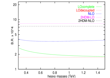
Figure 6: $BR(B\rightarrow X_{s}\gamma)$ as a function of $\mu_{\tilde{g}}$ for the parameters: $\tan\beta=1$, $m_{H^{\pm}}=m_{\tilde{t}_{2}}=m_{\chi_{2}}=100$ GeV, $m_{\chi_{1}}=300$ GeV, $\theta_{\tilde{t}}=-\pi/10$, $A_{b}=A_{t}$; all heavy particle masses equal to $\mu_{\tilde{g}}$; the lighter chargino is predominantly higgsino. Figure taken from M. Ciuchini et al. [4]

The NLO result for the combination of the charged-Higgs and the chargino contribution is represented by the middle curve.

This calculation, however, cannot be used in particular directions of the parameter space of the above listed models in which quantum effects induce a gluino contribution as large as the chargino or the SM contributions. Nor it can be used as a model-discriminator tool, able to constrain the potentially large sources of flavour violation typical of generic supersymmetric models.

The flavour non diagonal vertex gluino-quark-squark induced by the flavour violating scalar mass term and trilinear terms is particularly interesting. This is generically assumed to induce the dominant contribution to quark flavour transitions, as this vertex is weighted by the strong coupling constant $g_{s}$. Therefore, it is often taken as the only contribution to these transitions and in particular to the $B\rightarrow X_{s}\gamma$ decay, when extracting order of magnitude upper bounds on flavour violating terms in the scalar potential [56, 57]. Once the constraints coming from the experimental measurements are imposed, however, the gluino contribution is reduced to values such that the SM and the other supersymmetric contributions cannot be neglected anymore. Any LO and NLO calculation of the $B\rightarrow X_{s}\gamma$ rate in generic supersymmetric models, therefore, should then include all possible contributions.

The gluino contribution, however, presents some peculiar features related to the implementation of the QCD corrections. In ref. [6] this contribution to the decay $b\rightarrow s\gamma$ is therefore investigated in great detail for supersymmetric models with generic soft terms. It is shown that the relavant operator basis of the SM effective Hamiltonian gets enlarged to contain magnetic and chromomagnetic operators with an extra factor of $\alpha_{s}$ and weighted by a quark mass $m_{b}$ or $m_{c}$, and also magnetic and chromomagnetic operators of lower dimensionality, as well as additional scalar and tensorial four-quark operators. A few results of the analysis in ref. [6] are given in the following, showing the effect of the LO QCD corrections on constraints on supersymmetric sources of flavour violation.

To understand the sources of flavour violation which may be present in supersymmetric models in addition to those enclosed in the CKM matrix, one has to consider the contributions to the squark mass matrices

$${\cal M}_{f}^{2}=\left(\begin{array}[]{cc}m^{2}_{f,LL}&m^{2}_{f,LR}\\ m^{2}_{f,RL}&m^{2}_{f,RR}\end{array}\right)+$$

$$\left(\begin{array}[]{cc}F_{f,LL}+D_{f,LL}&F_{f,LR}\\ F_{f,RL}&F_{f,RR}+D_{f,RR}\end{array}\right)\quad,$$

where $f$ stands for up- or down-type squarks. In the super CKM basis where the quark mass matrices are diagonal and the squarks are rotated in parallel to their superpartners, the $F$ terms from the superpotential and the $D$ terms turn out to be diagonal $3\times 3$ submatrices of the $6\times 6$ mass matrices ${\cal M}^{2}_{f}$. This is in general not true for the additional terms (4), originating from the soft supersymmetry breaking potential. As a consequence, gluino contributions to the decay $b\rightarrow s\gamma$ are induced by the off-diagonal elements of the soft terms $m^{2}_{f,LL}$, $m^{2}_{f,RR}$, $m^{2}_{f,LR}$ and $m^{2}_{f,RL}$.

It is convenient to select one possible source of flavour violation in the squark sector at a time and assume that all the remaining ones are vanishing. Following ref. [56], all diagonal entries in $m^{2}_{\,d,\,LL}$, $m^{2}_{\,d,\,RR}$, and $m^{2}_{\,u,\,RR}$ are set to be equal and their common value is denoted by $m_{\tilde{q}}^{2}$. The branching ratio can then be studied as a function of

$$\delta_{LL,ij}=\frac{(m^{2}_{\,d,\,LL})_{ij}}{m^{2}_{\tilde{q}}}\,,\hskip 2.84544pt\delta_{RR,ij}=\frac{(m^{2}_{\,d,\,RR})_{ij}}{m^{2}_{\tilde{q}}}\,,\hskip 2.84544pt$$ (21)

$$\delta_{LR,ij}=\frac{(m^{2}_{\,d,\,LR})_{ij}}{m^{2}_{\tilde{q}}}\,,\,(i\neq j).$$ (22)

The remaining crucial parameter needed to determine the branching ratio is $x=m^{2}_{\tilde{g}}/m^{2}_{\tilde{q}}$, where $m_{\tilde{g}}$ is the gluino mass. In the following, we concentrate on the LO QCD corrections to the gluino contribution.

Figure 7: Gluino-induced branching ratio $BR(B\rightarrow X_{s}\gamma)$ as a function of $x=m^{2}_{\tilde{g}}/m^{2}_{\tilde{q}}$, obtained when the only source of flavour violation is $\delta_{LR,23}$ (see text).

Figure 8: Same as in Fig. 7 when only $\delta_{LL,23}$ is non-vanishing.

In Figs. 7 and 8, the solid lines show the QCD corrected branching ratio, when only $\delta_{LR,23}$ or $\delta_{LL,23}$ are non vanishing. The branching ratio is plotted as a function of $x$, using $m_{\tilde{q}}=500\,$GeV. The dotted lines show the range of variation of the branching ratio, when the renormalization scale $\mu_{b}$ varies in the interval $2.4$–$9.6\,$GeV. Numerically, the scale uncertaintly in $BR(B\rightarrow X_{s}\gamma)$ is about $\pm 25\%$. An extraction of bounds on the $\delta$ quantities more precise than just an order of magnitude, therefore, would require the inclusion of NLO QCD corrections. It should be noticed, however, that the inclusion of the LO QCD corrections has already removed the large ambiguity on the value to be assigned to the factor $\alpha_{s}(\mu)$ in the gluino-induced operators. Before adding QCD corrections, the scale in this factor can assume all values from $O(m_{b})$ to $O(m_{W})$: the difference between $BR(B\rightarrow X_{s}\gamma)$ obtained when $\alpha_{s}(m_{b})$ or when $\alpha_{s}(m_{W})$ is used, is of the same order as the LO QCD corrections. The corresponding values for $BR(B\rightarrow X_{s}\gamma)$ for the two extreme choices of $\mu$ are indicated in Figs. 7 and 8 by the dot-dashed lines ($\mu=m_{W}$) and the dashed lines ($\mu=m_{b}$). The choice $\mu=m_{W}$ gives values for the non-QCD corrected $BR(B\rightarrow X_{s}\gamma)$ relatively close to the band obtained when the LO QCD corrections are included, if only $\delta_{LL,23}$ is non-vanishing. Finding a corresponding value of $\mu$ that minimizes the QCD corrections in the case studied in Fig. 7, when only $\delta_{LR,23}$ is different from zero, depends strongly on the value of $x$. In the context of the full LO result, it is important to stress that the explicit $\alpha_{s}$ factor has to be evaluated - like the Wilson coefficients - at a scale $\mu=O(m_{b})$.

In spite of the large uncertainties which the branching ratio $BR(B\rightarrow X_{s}\gamma)$ still has at LO in QCD, it is possible to extract indications on the size that the $\delta$-quantities may maximally acquire without inducing conflicts with the experimental measurements (see [6]).

5 Summary

Significant progress in the theoretical description of rare B decays has been achieved during the last few years. NLO QCD corrections are available for radiative inclusive decays in the SM. Power correction ($1/m_{b}^{2}$, $1/m_{c}^{2}$) are also under control. The description of the Fermi motion of the $b$ quark in the $B$ meson has been refined. Important NNLO QCD improvement of the matching conditions of the operators relevant for $B\rightarrow X_{s}\ell^{+}\ell^{-}$ was made, which removes the $\pm 16\%$ matching scale uncertainty in the invariant mass distribution of the lepton pair. In some regions of the parameter space, NLO QCD corrections to $BR(B\rightarrow X_{s}\gamma)$ in 2HDMS are huge. They are, however, under control in the type-II model and are important to derive reliable bounds on $\tan\beta$ and $m_{H^{\pm}}$. NLO QCD corrections to $BR(B\rightarrow X_{s}\gamma)$ are available also in particular SUSY scenarios. Calculations for more general situations are in progress.

- [1] A. Masiero, talk at this meeting.
- [2] F. Borzumati and C. Greub, Phys. Rev. D 58 (1998) 074004.
- [3] M. Ciuchini, G. Degrassi, P. Gambino and G.F. Giudice, Nucl. Phys. B 527 (1998) 21.
- [4] M. Ciuchini, G. Degrassi, P. Gambino and G.F. Giudice, Nucl. Phys. B 534 (1998) 3.
- [5] C. Bobeth, M. Misiak and J. Urban, hep–ph/9904413.
- [6] F. Borzumati, C. Greub, T. Hurth and D. Wyler, hep–ph/9911245.
- [7] A.F. Falk, M. Luke and M. Savage, Phys. Rev. D 49 (1994) 3367.
- [8] M.B. Voloshin, Phys. Lett. B 397 (1997) 295; A. Khodjamirian, R. Rückl, G. Stoll and D. Wyler, Phys. Lett. B 402 (1997) 167; Z. Ligeti, L. Randall and M.B. Wise, Phys. Lett. B 402 (1997) 178; A.K. Grant, A.G. Morgan, S. Nussinov and R.D. Peccei, Phys. Rev. D 56 (1997) 3151;
- [9] G. Buchalla, G. Isidori and S.J. Rey, Nucl. Phys. B 511 (1998) 594.
- [10] V. Braun, talk at this meeting; hep–ph/9911206.
- [11] L. Silvestrini, talk at this meeting; hep–ph/9911269.
- [12] D.E. Jaffe, talk at this meeting; hep–ex/9910055.
- [13] M. Ciuchini, E. Franco, G. Martinelli, L. Reina and L. Sivestrini, Phys. Lett. B 316 (1993) 127; Nucl. Phys. B 415 (1994) 403; G. Cella, G. Curci, G. Ricciardi and A. Vicere, Phys. Lett. B 325 (1994) 227.
- [14] K. Adel and. Y.-P. Yao, Phys. Rev. D 49 (1994) 4945.
- [15] C. Greub and T. Hurth,Phys. Rev. D 56 (1997) 2934.
- [16] A.J. Buras, A. Kwiatkowski and N. Pott, Nucl. Phys. B 517 (1998) 353; Phys. Lett. B 414 (1997) 157, E:ibid. 434 (1998) 459.
- [17] K. Chetyrkin, M. Misiak and M. Münz, Phys. Lett. B 400 (1997) 206.
- [18] A. Ali and C. Greub, Z. Physik C 49 (1991) 431; Phys. Lett. B 259 (1991) 182; Z. Physik C 60 (1993) 433; Phys. Lett. B 361 (1995) 146.
- [19] N. Pott, Phys. Rev. D 54 (1996) 938.
- [20] C. Greub, T. Hurth and D. Wyler, Phys. Lett. B 380 (1996) 385; Phys. Rev. D 54 (1996) 3350.
- [21] A. Czarnecki and W.J. Marciano, Phys. Rev. Lett. 81 (1998) 277.
- [22] A.L. Kagan and M. Neubert, Eur. Phys. J.C7 (1999) 5.
- [23] A. Strumia, Nucl. Phys. B 532 (1998) 28.
- [24] K. Baranowski and M. Misiak, hep-ph/9907427.
- [25] F. Borzumati and C. Greub, Phys. Rev. D 59 (1999) 057501 and hep–ph/9810240.
- [26] R. Barate et al. (ALEPH Collab.), Phys. Lett. B 429 (1998) 169.
- [27] S. Ahmed et al. (CLEO Collab.) CLEO CONF 99-10, hep-ex/9908022.
- [28] A. Ali and C. Greub, Phys. Lett. B 293 (1992) 226.
- [29] G. Altarelli et al., Nucl. Phys. B 208 (1982) 365; A. Ali and E. Pietarinen, Nucl. Phys. B 154 (1979) 519.
- [30] M. Neubert, Phys. Rev. D 49 (1994) 3392 and 4623; I.I. Bigi, M.A. Shifman, N.G. Uraltsev and A.I. Vainshtein, Int. J. Mod. Phys. A 9 (1994) 2467; R. D. Dikeman, M. Shifman and N.G. Uraltsev, Int. J. Mod. Phys. A 11 (1996) 571; T. Mannel and M. Neubert, Phys. Rev. D 50 (1994) 2037.
- [31] M. Gremm, A. Kapustin, Z. Ligeti and M.B. Wise, Phys. Rev. Lett. 77 (1996) 20.
- [32] M.S. Alam et al. (CLEO Collab.), Phys. Rev. Lett. 74 (1995) 2885.
- [33] A.K. Leibovich and I.Z. Rothstein, hep–ph/9907391.
- [34] Z. Ligeti, M. Luke, A.V. Manohar, and M.B. Wise, Phys. Rev. D 60 (1999) 034019.
- [35] C. Greub and T. Hurth, Nucl. Phys. B74 (Proc. Suppl.) (1999) 247.
- [36] A. Ali, A. Asatrian and C. Greub, Phys. Lett. B 429 (1998) 87.
- [37] A. Ali, C. Greub and T. Mannel, report DESY 93-016, published in the Proc. of the ECFA Workshop on a European B Meson Factory, Eds. R. Aleksan and A. Ali, Hamburg 1993.
- [38] G. Buchalla and A.J. Buras, Nucl. Phys. B 400 (1993) 225.
- [39] ALEPH Collaboration, Contributed paper (PA10-019) to the 28th. International Conference on High Energy Physics, Warsaw, 1996.
- [40] M. Misiak, Nucl. Phys. B 393 (1993) 23; [E: ibid. 439 (1995) 461].
- [41] A.J. Buras and M. Münz, Phys. Rev. D 52 (1995) 186.
- [42] A. Ali and G. Hiller, Eur. Phys. J.C8 (1999) 619.
- [43] C. Bobeth, M. Misiak and J. Urban, hep–ph/9910220.
- [44] M. Krawczyk and J. Zochowski, Phys. Rev. D 55 (1997) 6968.
- [45] F. Borzumati and A. Djouadi, hep–ph/9806301.
- [46] see for example: F. Borzumati, hep–ph/9702307.
- [47] P. Ciafaloni, A. Romanino, and A. Strumia, Nucl. Phys. B 524 (1998) 361.
- [48] P. Janot, in “International Europhysics Conference on HEP 1997”, Jerusalem (Israel), August 1997.
- [49] M. Krawczyk, P. Mättig, and J. Zochowski, Eur. Phys. J.C8 (1999) 495.
- [50] A.H. Chamseddine, R. Arnowitt and P. Nath, Phys. Rev. Lett. 49 (1982) 970; R. Barbieri, S. Ferrara, and C.A. Savoy, Phys. Lett. B 119 (1982) 343; L.J. Hall, J. Lykken, and S. Weinberg, Phys. Rev. D 27 (1983) 2359.
- [51] M. Dine, W. Fischler, and M. Srednicki, Nucl. Phys. B 189 (1981) 575; S. Dimopoulos and S. Raby, Nucl. Phys. B 192 (1981) 353; M. Dine and A.E. Nelson, Phys. Rev. D 49 (1993) 1277; M. Dine, A.E. Nelson, and Y. Shirman, Phys. Rev. D 51 (1995) 1362; M. Dine, A.E. Nelson, Y. Nir and Y. Shirman, Phys. Rev. D 53 (1996) 2658.
- [52] M. Leurer, Y. Nir, and N. Seiberg, Nucl. Phys. B 398 (1993) 319; ibid. 420 (1994) 468.
- [53] T. Goto, Y. Okada and Y. Shimizu, Phys. Rev. D 58 (1998) 094006.
- [54] F.M. Borzumati, M. Olechowski and S. Pokorski, Phys. Lett. B 349 (1995) 311; F.M. Borzumati, hep-ph/9702307.
- [55] S. Bertolini, F. Borzumati, A. Masiero, and G. Ridolfi, Nucl. Phys. B 353 (1991) 591.
- [56] F. Gabbiani, E. Gabrielli, A. Masiero, and L. Silvestrini, Nucl. Phys. B 477 (1996) 321.
- [57] J.S. Hagelin, S. Kelley, and T. Tanaka, Nucl. Phys. B 415 (1994) 293.