Flavour Physics: the questions, the clues and the challenges

Abstract

Flavour physics addresses some of the questions for which the Standard Model does not provide a satisfactory and complete answer: the origin of the replication of the fundamental constituents and of their mass hierarchy. This paper reviews some of the theoretical approaches and the experimental strategies that can lead us to a more complete picture. Results included in this review are $|V_{cb}|=0.0382\pm 0.0032$, $|V_{ub}/V_{cb}|=0.085\pm 0.023$ and a preliminary measurement of the branching fraction of $B\rightarrow\pi^{+}\pi^{-}=(0.47^{+0.18}_{-0.15}\pm 0.06)\times 10^{-5}$.

1 Introduction

The subject of flavour physics is a vast one and I am not going to review the entire body of present knowledge. Instead, I would like to use a few examples to define the problems that we are struggling with and the strategies that we can use to reach a deeper understanding of this elusive subject.

Our main puzzle was concisely and effectively put by I.I. Rabi upon the discovery of the $\mu$: “Who ordered that?” was his remark. This question has three distinctive facets. We can start by asking the reason why there are so many particles: this can be defined as the “replication problem.” Once we organize the particles in the Standard Model families we have a triplication problem: “Why are there three families?” Finally, the hierarchy in the mass spectrum of quarks and leptons spans several orders of magnitudes and may provide the most distinct clue towards an answer to Rabi’s puzzling question. Even if lepton masses and mixing parameters have recently attracted a lot of attention, because of the evidence for $\nu$ oscillations from the Super-Kamiokande experiment, the quark sector will be the focus of my discussion. Masses and mixing in the lepton sector are reviewed in other excellent contributions to these proceedings [1].

In the Standard Model masses are produced via the Higgs mechanism through the Yukawa couplings. The Yukawa Lagrangian is given by:

$$\begin{array}[]{ll}{\cal L}_{Yukawa}=&-G_{1}[(\overline{L}_{u}\overline{\Phi})u_{R}+\overline{u}_{R}(\overline{\Phi}^{\dagger}L_{u})]\\ {}{}&-G_{2}[(\overline{L}_{u}\overline{\Phi})d_{R}+\overline{d}_{R}(\overline{\Phi}^{\dagger}L_{u})]\\ {}{}&-G_{3}[(\overline{L}_{u}\overline{\Phi})s_{R}+\overline{s}_{R}(\overline{\Phi}^{\dagger}L_{u})]\\ {}{}&-G_{4}[(\overline{L}_{c}\overline{\Phi})c_{R}+\overline{c}_{R}(\overline{\Phi}^{\dagger}L_{c})]\\ {}{}&-G_{5}[(\overline{L}_{c}\overline{\Phi})d_{R}+\overline{d}_{R}(\overline{\Phi}^{\dagger}L_{c})]\\ {}{}&-G_{6}[(\overline{L}_{c}\overline{\Phi})s_{R}+\overline{s}_{R}(\overline{\Phi}^{\dagger}L_{c})],\\ \end{array}$$ (1)

where $L$ identifies a left-handed SU(2) doublet and the subscript $R$ identifies a right-handed fermion. These 6 complex Yukawa couplings are related to 10 independent physical quantities, the six quark masses and four quark mixing parameters. The latter can be described by three Euler-like angles and an imaginary phase. These parameters are not predicted by the Standard Model, but are fundamental constants of nature that need to be extracted from experimental data.

Many theoretical models have tried to uncover a more fundamental explanation for flavour. For example, some of the many variations of Supersymmetry [2] incorporate the known hierarchy of quark masses and mixing parameters. In addition, the replication problem has been addressed by postulating a new deeper level of matter [3]. In this approach, the multitude of quarks can be understood as a sort of periodic table of the composite structures that are indeed bound states of more fundamental particles. In addition, a geometrical origin [4] of flavor has been proposed.

An additional feature of the fundamental interactions explored in flavour physics is $CP$ violation. The only experimental evidence has been obtained studying neutral $K$ decays. On the other hand, $CP$ violation is crucial to our understanding of the history of the universe. In particular, it is a necessary ingredient of our understanding of the origin of the matter dominated universe [5]. A $CP$ violating phase is naturally incorporated in the Standard Model within the Cabibbo- Kobayashi-Maskawa matrix. Thus several models attempt to explain the baryon asymmetry of the universe as due to a $CP$ violating process occurring at the scale of the electroweak symmetry breaking. A rough order of magnitude estimate of the expected effect of the CKM induced $CP$ violation on the baryon asymmetry can be obtained by constructing a variable $d_{CP}$ that incorporates all the features of the expected CKM phase: it vanishes when any pair of quarks is degenerate in mass and when any CKM angle vanishes because of the so called “GIM” (Glashow, Iliopoulos, Maiani) cancellation. $d_{CP}$ is defined as:

$$\begin{array}[]{ll}d_{CP}=&\sin{\theta_{12}}\sin{\theta_{23}}\sin{\theta_{13}}\sin{\delta_{CP}}\\ {}{}&(m_{t}^{2}-m_{c}^{2})(m_{t}^{2}-m_{u}^{2})(m_{c}^{2}-m_{u}^{2})\\ {}{}&(m_{b}^{2}-m_{s}^{2})(m_{b}^{2}-m_{d}^{2})(m_{s}^{2}-m_{d}^{2}),\\ \end{array}$$ (2)

where $\theta_{ij}$ are three real “Euler-like” angles defining the CKM matrix together with the imaginary phase $\delta_{CP}$.

The $d_{CP}$ parameter that we have just defined is a dimensional quantity, it is conceivable [6] that the natural normalization parameter to transform it into a pure number is the temperature at which the electroweak symmetry breaking occurred. Thus the figure of merit of the strength of the CKM induced CP violating effect is given by:

$$d_{CP}^{T}=d_{CP}/kT_{ew}^{12}\approx 10^{-18},$$ (3)

where $T_{ew}$ represents the temperature at the time the electroweak symmetry breaking occurred and $k$ is the Boltzmann constant. This suggests that CKM CP violation is an effect too small to account for the known baryon asymmetry of the universe,

$$\left|\frac{N_{B}-N_{\overline{B}}}{N_{B}+N_{\overline{B}}}\right|_{t\approx 10^{-6}s}\approx\left|\frac{N_{B}}{N_{\gamma}}\right|_{now}\approx 10^{-10}.$$ (4)

This discrepancy is very qualitative in nature and may have a number of explanations. However a very tantalizing hypothesis is the presence of additional $CP$ violating phases produced by mechanisms beyond the Standard Model. Thus, the experimental exploration of $CP$ violation observables has a good chance to uncover evidence for new physics.

2 Quark Masses

The hierarchy of the quark masses is very puzzling. The mass interval between the lightest and the heaviest quark spans the huge interval between a few MeV and hundreds of GeV. The determination of these masses has many challenges and a good illustration of the different roles played by QCD in different hadronic processes. The parameter that defines how QCD affects our ability of measuring fundamental properties is the mass scale $\Lambda_{QCD}\approx 500$ MeV. Thus, for very heavy mass scales QCD corrections are not very important and can be evaluated using perturbative methods. As the mass decreases, non-perturbative effects become more important and the extrapolation process becomes more uncertain. This interplay will be illustrated below.

2.1 The top quark mass

The top quark is the heaviest and thus the least affected by the strong interaction. In fact, it is so heavy that it has the unique property of decaying before hadronizing in a top-flavored hadron. It was discovered at Fermilab [7], at the Tevatron proton-antiproton collider. Its properties have been studied by CDF and D0. In particular, one of the finest achievements by these groups is a very accurate determination of the quark mass $m_{t}$. Several different techniques are used. Recently, these two experiments have formed a working group to obtain a world average for $m_{t}$, considering the correlations in their measurements.

The top quark decays into a $b$ quark and a $W$ boson with a probability close to one. In some cases this $b$ quark undergoes semileptonic decays. In both CDF and D0 the dominant contribution to the $m_{t}$ measurement comes from samples containing one high $p_{t}$ lepton and one jet. CDF also uses a sample including only hadrons in the final state, whereas D0 has a secondary data set containing two leptons.

The value of the measured top quark mass is $(174.3\pm 3.2\pm 4.0)$ GeV. This is the heaviest measured mass of a fundamental particle. The interest in studying the properties of the top quark is largely motivated by the unique closeness of $m_{t}$ to the mass defining the scale of the electroweak symmetry breaking. The mass $m_{t}$ is related to the vacuum expectation value of the Higgs field through the relationship:

$$m_{t}=\lambda_{t}v/\sqrt{2},$$ (5)

where $\lambda_{t}$ is the Yukawa coupling and $v$ is the vacuum expectation value of the Higgs field. Note that the Yukawa coupling is of order one. This property can be accomodated in a natural way in some supersymmetric theories that encompass a very heavy top quark at the GUT scale [8].

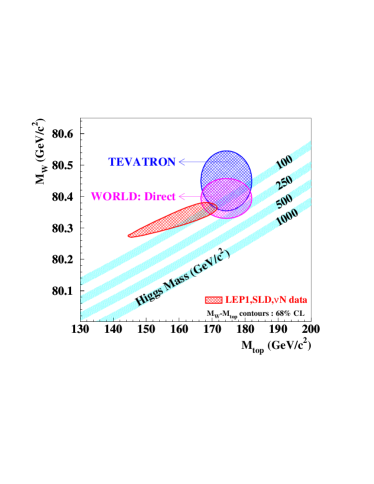
Figure 1: Relation between the W and top masses for some values of the Higgs mass [9]. The cross hatched area to the left represents the allowed region from an overall Standard Model fit. The other two regions are obtained from direct measurements of M_W and M_top.

The measured $W$ and top masses can give some constraint on the mass scale for the last particle in the Standard Model to elude our discovery, the Higgs scalar. Fig. 1 shows a summary of the constraints on the Higgs mass from the $W$ mass measurements at LEP II and the combined $m_{W}$ and $m_{t}$ at the Tevatron. These data favor a light Higgs, leading to the hope that we are on the verge of learning more about the mechanism of electroweak symmetry breaking.

2.2 The $b$ quark mass

The interest in an accurate measurement of the $b$ quark mass has a two-fold motivation. On the one hand its measurement helps to pin down the quark mass hierarchy as discussed before. On the other hand, renewed attention to $m_{b}$ has been motivated by the suggestion that the CKM matrix elements $|V_{cb}|$ and $|V_{ub}|$ can now be obtained from inclusive measurements with great accuracy using the so called “Heavy Quark Expansion” [10]. A precise determination of $m_{b}$ is a “sine qua non” for most inclusive methods to study $B$ decays. Since the mass of the beauty quark is about 5 GeV, thus its derivation from experimental observables is affected by the strong interaction to a much higher degree that in the $t$ quark case. In fact, before we discuss any theoretical estimate or experimental determination of the $b$ quark mass we need to define its meaning carefully. The widely used “pole mass,” namely the parameter appearing in the quark propagator, has been demonstrated to be inadequate [11] for an accurate description of $b$ quark phenomenology. These authors point out the existence of an infrared renormalon generating a factorial divergence in the high-order cofficients in the $\alpha_{S}$ series producing an intrinsic uncertainty of the order $\Lambda_{QCD}/m_{Q}$.

An alternative, that appears to be quite a good candidate to describe $b$ quark properties in a regime where perturbative effects are important, is the $\overline{MS}$ mass $\overline{m}_{b}(\mu)$. This is a short distance mass, and therefore does not contain ambiguities of the order of $\Lambda_{QCD}$ like the pole mass. This definition is adequate for observables where perturbative effects are dominant, such as recent measurements of the $b$ quark mass at the $Z^{0}$ energy. As this quantity is not defined for scales $\mu$ below $m_{b}$, alternative definitions of the running mass have been proposed that can be normalized at a scale $\mu$ smaller than $m_{b}$. Most of the authors refer to the mass defined with this procedure as “kinetic mass.”

Table 1 summarizes the most recent theoretical evaluations of $m_{b}$. The calculations using the $m_{kin}$ prescription or an equivalent subtraction scheme are in closer agreement. However other evaluations of the pole mass and the $\overline{MS}$ mass have shown frequent disagreement in the methodology of assessing errors. In addition, recent lattice data [13] seem to imply an even lighter $m_{b}$. It is clear that there is still work to be done before quantities sensitive to $m_{b}$ can be determined accurately.

Table 1: Theoretical estimates of $m_{b}$ (GeV/c²). The first column gives the theoretical predictions for the pole mass $m_{b}$, the second column the predicted value of the $\overline{MS}$ mass $\overline{m}_{b}(m_{b})$ at the scale of the $b$ meson mass and the third column corresponds to the prediction for the kinetic or potential subtracted mass defined at a scale $\mu\approx 1$ GeV.

$m_{b}$	$\overline{m}_{b}$	$m_{kin}$	Ref.
QCD sum rule evaluations
–	$4.20\pm 0.1$	$4.56\pm 0.06$	[14]
–	$4.20\pm 0.06$	$4.71\pm 0.06$	[15]
$4.97\pm 0.17$	$4.26\pm 0.12$	$4.60\pm 0.18$	[16]
$4.75\pm 0.04$	–	–	[17]
$\Upsilon$ sum rule evaluations
$4.604\pm 0.014$	$4.13\pm 0.06$	–	[18]
$5.015^{+0.110}_{-0.070}$	$4.453^{+0.050}_{-0.032}$	–	[19]
Lattice QCD evaluations
$5.0\pm 0.2$	$4.0\pm 0.1$	–	[20]
–	$4.41\pm 0.15$	–	[21]

3 Quark Mixing

In the framework of the Standard Model the gauge bosons, $W^{\pm}$, $\gamma$ and $Z^{o}$ couple to mixtures of the physical $d,~{}s$ and $b$ states. This mixing is described by the Cabibbo-Kobayashi-Maskawa (CKM) matrix:

$$V_{CKM}=\left(\begin{array}[]{ccc}V_{ud}&V_{us}&V_{ub}\\ V_{cd}&V_{cs}&V_{cb}\\ V_{td}&V_{ts}&V_{tb}\end{array}\right).$$ (6)

A commonly used approximate parameterization was originally proposed by Wolfenstein [22]. It reflects the hierarchy between the magnitude of matrix elements belonging to different diagonals. It is:

$$\scriptsize{\begin{array}[]{ccc}1-\lambda^{2}/2&\lambda&A\lambda^{3}(\rho-i\eta(1-\lambda^{2}/2))\\ -\lambda&1-\lambda^{2}/2-i\eta A^{2}\lambda^{4}&A\lambda^{2}(1+i\eta\lambda^{2})\\ A\lambda^{3}(1-\rho-i\eta)&-A\lambda^{2}&1\end{array}}$$ (7)

The CKM matrix must be unitary and the relation between elements of different rows dictated by this property can be graphically represented as so called ‘unitarity triangles’. Fig. 2 shows the 6 unitarity triangles that can be constructed to check this property. The expected lengths of the sides are suggested. The bottom two triangles give a hint on the optimal strategy to test the CKM sector of the Standard Model. The three sides are of comparable length and thus all the angles and sides are more amenable to experimental measurement. The CKM matrix is characterized by four independent parameters. Aleksan, Kayser and London [23] pointed out that we can express the CKM matrix as a function of four phases that can be determined by $CP$ observables. These phases are:

$$\beta=arg\left(-\frac{V_{tb}V_{ts}^{\star}}{V_{cb}V_{cd}^{\star}}\right)$$ (8)

$$\gamma=arg\left(-\frac{V_{ub}^{\star}V_{ud}}{V_{cb}^{\star}V_{cd}}\right)$$ (9)

$$\chi=arg\left(-\frac{V_{cs}^{\star}V_{cb}}{V_{ts}^{\star}V_{tb}}\right)$$ (10)

$$\chi^{\prime}=arg\left(-\frac{V_{ud}^{\star}V_{us}}{V_{cd}^{\star}V_{cs}}\right)$$ (11)

Silva and Wolfenstein [24] emphasized that we can use these phases to identify new physics effects in $B$ decays. The details of an experimental program capable of making these measurements with the needed accuracy will be discussed below.

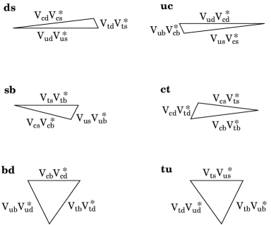
Figure 2: The six CKM triangles. The bold labels, i.e ds refer to the rows or columns used in the unitarity relationship.

The experimental information presently available consists of $CP$ violation observables in the $K$ system, discussed by G. Buchalla [25] in these proceedings, and by a variety of constraints on the sides of the unitarity triangles. Very often the dominant uncertainty in the extraction of the magnitude of the CKM parameters from the data is the relationship between experimental observables and the quark mixing parameter to be measured. This relationship is governed by a matrix element involving strong interaction effects. The challenges and possible pitfalls in the evaluation of the relevant matrix elements are discussed below.

3.1 The determination of $V_{cb}$ from the decay $B\rightarrow D^{\star}\ell\overline{\nu}$.

Heavy Quark Effective Theory (HQET) [26] has been a very important breakthrough in our understanding of $B$ meson decays. It is an effective theory that gives very definite predictions in the limit of infinite quark masses. In addition, corrections for finite quark masses can be accounted for with a systematic study of non-perturbative effects using a 1/$m_{Q}$ expansion, where $m_{Q}$ represents the mass of the heavy quarks involved in the process. One of the first implication of the theory [27] has been the advantage offered by the decay $B\rightarrow D^{\star}\ell\nu$. The differential decay width $\Gamma(B\rightarrow D^{\star}\ell\overline{\nu})$ is a function of the invariant 4-velocity transfer $w=\vec{v}\cdot\vec{v^{\prime}}$, where $\vec{v}$ and $\vec{v^{\prime}}$ are the 4-velocities of the incoming and outgoing heavy hadron respectively. It is given by:

$$\frac{d\Gamma}{dw}={\cal K}(w){\cal F}^{2}(w)|V_{cb}|^{2},$$ (12)

$${\cal F}(w)={\cal F}_{D^{\star}}(1){\cal G}(w)$$ (13)

where ${\cal K}(w)$ is a known phase space factor, ${\cal G}(w)$ is the shape of the Isgur-Wise function and ${\cal F}_{D^{\star}}(1)$ is a normalization factor that is predicted from this effective theory. It is generally expressed as:

$${\cal F}(1)=\eta_{A}(1+const\times\frac{\Lambda_{QCD}^{2}}{m_{Q}^{2}}+\cdots)$$ (14)

$$\equiv\eta_{A}(1+\delta_{1/m_{Q}^{2}})$$

Note, the $1/m_{Q}$ term vanishes. The parameter $\eta_{A}$ is the short distance correction arising from the finite renormalization of the flavour changing axial current at zero recoil and $\delta_{1/m_{Q}^{2}}$ parametrizes the second order term (and higher) order corrections in the $1/m_{Q}$ expansion including the effects of finite heavy quark masses. There has been a lot of theoretical activity on both $\eta_{A}$ and $1/m_{Q}^{2}$ corrections. The $\eta_{A}$ factor has been calculated by Czarnecki at two loop order [28] to be $0.960\pm 0.007$. The $1/m_{Q}^{2}$ correction has been evaluated in different approaches and is more subjected to the author bias because it involves non-perturbative effects [29], [30], [31], [32], [33]. These different estimates have been combined into [34]:

$${\cal F}(1)=0.913\pm 0.007\pm 0.024\pm 0.011,$$ (15)

where the first error accounts for the remaining perturbative uncertainty, the second one reflects the uncertainty in the calculation of the $1/m_{Q}^{2}$ corrections and the third one gives an estimate of the higher-order power corrections. A very interesting recent development is that Lattice Gauge theory has produced a preliminary result on ${\cal F}(1)$. They obtain [35], [36] :

$${\cal F}(1)=0.935\pm 0.022^{+0.008}_{-0.011}\pm 0.008\pm 0.020,$$ (16)

where the first error is statistical, the second is due to the uncertainty in the quark masses, the third is the uncertainty in radiative corrections beyond 1 loop and the last represent $1/m_{Q}^{3}$ effects. Errors not yet estimated include the sensitivity to the lattice spacing adopted and to the quenching approximation. The calculation is in its initial stage, but this is a promising hint that an accurate value for ${\cal F}(1)$ will be available soon.

The present status of the experimental determination of the product ${\cal F}(1)V_{cb}$ is summarized in Table 2.

Table 2: Determination of $|V_{cb}|$ from $B\rightarrow D^{\star}\ell\overline{\nu}$. The first error in the $|V_{cb}|$ estimate is the experimental error, obtained adding in quadrature statistical and systematic errors. The last error is due to theoretical uncertainties in ${\cal F}(1)$.

Experiment	${\cal F}(1)V_{cb}\times 10^{-3}$	$V_{cb}\times 10^{-3}$
ALEPH [37]	$31.9\pm 1.8\pm 1.9$	$34.9\pm 2.9\pm 1.6$
DELPHI[38]	$37.7\pm 1.7\pm 1.7$	$41.3\pm 2.6\pm 1.9$
OPAL[39]	$32.8\pm 1.9\pm 2.2$	$35.9\pm 3.2\pm 1.5$
CLEO $\dagger$	$36.1\pm 1.9\pm 1.9$	$39.5\pm 2.9\pm 1.8$
AVERAGE	$34.8\pm 0.91\pm 0.95$	$38.2\pm 1.4\pm 1.8$

$\dagger$ The published CLEO result [40] has been scaled up by 3% according to the calculation performed by Stone [41] to account for the curvature of the form factor.

If we average these results, we obtain $V_{cb}=(38.2\pm 1.40_{exp}+1.8_{th})\times 10^{-3}$. The experimental error is obtained by adding in quadrature the statistical and systematic errors. The theoretical error is based on Eq. 16.

3.2 The determination of $|V_{cb}|$ from inclusive semileptonic decays.

An alternative determination of $V_{cb}$ has been obtained using the inclusive semileptonic branching fraction. This quantity has been studied both at the $\Upsilon({\rm 4S})$ from CLEO and ARGUS and at LEP. The most accurate measurement at the $\Upsilon({\rm 4S})$ has been reported by CLEO from a small subset of their full data sample [42] using a lepton tagged sample. This method of extracting the branching fraction is less model dependent as it can measure a larger portion of the electron spectrum as shown in Fig.  3.

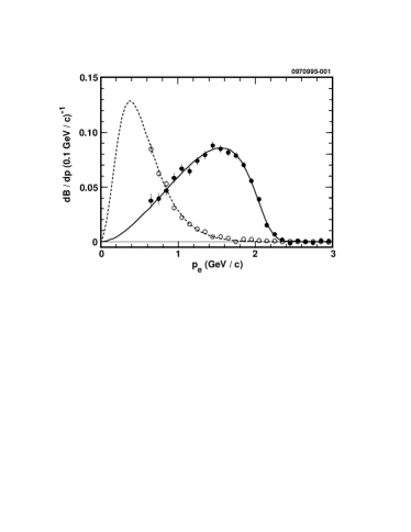
Figure 3: Spectra of electrons from $B\rightarrow Xe\overline{\nu}$ (filled circles) and $b\rightarrow c\rightarrow yl\overline{\nu}$ (open circles) identified with lepton tags. The curves show the best fit to the modified ISGW model, with 23% $B\rightarrow D^{\star\star}\ell\overline{\nu}$.

All the four LEP experiments reported measurements of the semileptonic branching fractions. The experimental information is summarized in Table 3. The measured semileptonic widths, obtained using the most recent average values for the $b$ quark and the $B$ meson lifetimes, are shown also. Note that the partial width measurements from LEP and the $\Upsilon({\rm 4S})$ are still mildly inconsistent. In addition, the systematic errors in different LEP experiments are evaluated using different methods and assumptions. A working group has been established to address this issue [43], but their work is still in progress. As the dominant error in these analyses is systematic, until these issues are settled it appears premature to use a weighted average of these results.

Table 3: Summary on semileptonic width data from CLEO and LEP. The lifetimes $\tau_{B}=1.605\pm 0.021$ ps and $\tau_{b}=1.564\pm 0.014$ ps are used to obtain $\Gamma_{SL}$ for CLEO and LEP respectively.

Exp.	${\cal B}_{SL}$(%)	$\Gamma_{SL}$
		$\times 10^{10}{\rm s}^{-1}$
ALPH [44]	$11.01\pm 0.10\pm 0.30$	$7.04{\scriptsize\pm 0.21}$
DPHI [45]	$10.65\pm 0.11\pm 0.23^{+0.43}_{-0.27}$	$6.81^{+0.32}_{-0.23}$
L3[46]	$10.16\pm 0.13\pm 0.29$	$6.50{\scriptsize\pm 0.20}$
OPAL[47]	$10.83\pm 0.10\pm 0.20^{+0.20}_{-0.13}$	$6.92^{+0.19}_{-0.17}$
CLEO[42]	$10.49\pm 0.17\pm 0.43$	$6.54{\scriptsize\pm 0.29}$

Recently proponents of the heavy quark expansion (HQE) [48] have suggested that inclusive quantities are the most promising avenue to perform a precise determination of the CKM parameters. The semileptonic width is related to $|V_{cb}|$ and to the matrix element calculated by HQE through:

$$\begin{array}[]{ll}|V_{cb}|=&0.0411\sqrt{{\cal B}(B\rightarrow X_{c}\ell\overline{\nu})/0.105}\\ {}{}&\times\sqrt{1.55/\tau_{B}({\rm ps})}\\ {}{}&\left[1-0.024\left(\frac{\mu_{\pi}^{2}-0.5}{0.1}\right)\right]\times\\ {}{}&(1\pm 0.01(pert.)\pm 0.01(m_{b})\\ {}{}&\pm 0.015(1/m_{b}^{3}))\end{array}$$ (17)

where $\mu_{\pi}^{2}$ is a kinetic energy contribution which is a gauge-covariant extension of the square of the $b$ quark momentum inside the heavy hadron, $\mu_{G}$ is the chromomagnetic matrix element defined to a given order in perturbative theory. Alternative formulations of this relationship have been proposed, either using slightly different parameterizations of the correction terms [49], or relating the semileptonic width to the $\Upsilon$ mass in order to reduce the uncertainties associated with quark masses [50]. If, for illustration purpose, we use the CLEO semileptonic width to extract $|V_{cb}|$ with this method, we obtain $|V_{cb}|=0.041\pm 0.001_{exp}\pm 0.0025_{th}$.

One very important concern is the dependence upon the quark masses. Bigi [51] assumes an uncertainty of 10%. Recent theoretical estimates of $m^{kin}_{b}$ seem to support this view, but more experimental data confirming this picture is needed. The semileptonic width in the heavy quark expansion is dependent upon $m_{c}$ and $m_{b}$ though the relationship:

$$\Gamma(B\rightarrow X_{c}\ell\overline{\nu})\propto G_{F}^{2}(m_{b}-m_{c})^{2}m_{b}^{3}$$ (18)

The difference $m_{b}-m_{c}$ can be inferred according to several authors [52] through the relationship:

$$\begin{array}[]{ll}m_{b}-m_{c}=&<M_{B}>-<M_{D}>+\\ {}{}&\mu^{2}_{\pi}\left(\frac{1}{2m_{c}}-\frac{1}{2m_{b}}\right)+\\ {}{}&{\cal O}(1/m_{b,c}^{2}),\end{array}$$ (19)

where $<M_{B}>$ and $<M_{D}>$ represent the spin averaged beauty and charm meson masses. This formula gives $m_{b}-m_{c}\approx 3.5$ GeV, corresponding to an uncomfortably low value of the $c$ quark mass [51].

Finally it is hard to give a reliable estimate of the possible quark hadron duality violation in inclusive decays. In fact there are some arguments that suggest a potential for significant violations of this assumption [53]. Until these issues are resolved, an average value of $|V_{cb}|$ based on the $D^{\star}\ell\overline{\nu}$ method and the inclusive semileptonic widths does not seem appropriate.

Additional experimental constraints are crucial to achieve a better understanding of these sources of errors. The study of the moments of the lepton spectrum and of the hadronic mass spectrum provides in principle an additional constraint that allows the extraction of some of the theoretical parameters described above from data. The moments of the hadronic mass spectrum are defined as:

$$<(s_{H}-\overline{m}_{D}^{2})^{n})>\equiv\frac{1}{\Gamma_{SL}}\int ds\frac{d\Gamma}{ds}(s-\overline{m}_{D}^{2})^{n},$$ (20)

where $s$ represent the hadronic mass recoiling against the lepton-neutrino pair and $\overline{m}_{D}$ represents the spin averaged mass of the $D$ meson. If we use the heavy quark expansion result for $\Gamma_{SL}$, we obtain for the first moment [49] :

$$\begin{array}[]{ll}<(s_{H}-\overline{m}_{D}^{2})>=&m_{B}^{2}[0.051\frac{\alpha_{S}}{\pi}+\\ {}{}&0.23\frac{\overline{\Lambda}}{m_{B}}(1+0.43\frac{\alpha_{S}}{\pi})\\ {}{}&+0.26\frac{\overline{\Lambda}^{2}}{m_{B}^{2}}+1.01\frac{\lambda_{1}}{m_{B}^{2}}\\ {}{}&-0.31\frac{\lambda_{2}}{m_{B}^{2}}]\end{array}$$ (21)

where the two matrix elements $\lambda_{1}$ and $\lambda_{2}$, characterizing the corrections of order $\Lambda_{QCD}/m_{b}^{2}$ are given by:

$$\lambda_{1}=-\frac{1}{2m_{B}}<B|\overline{h}_{\nu}(i\vec{D})^{2}h_{\nu}|B>,$$ (22)

$$\lambda_{2}=\frac{1}{3}<B|\overline{h}_{\nu}\frac{g}{2}\sigma_{\mu\nu}G^{\mu\nu}h_{\nu}|B>,$$ (23)

where $h_{\nu}$ is the heavy quark field in the effective theory with velocity $\vec{v}$. The parameter $\overline{\Lambda}$ is related to the $b$ quark mass through the relationship:

$$m_{B}=m_{b}+\overline{\Lambda}-\frac{\lambda_{1}+3\lambda_{2}}{2m_{b}}.$$ (24)

The $B^{\star}-B$ mass splitting determines $\lambda_{2}=0.12\ {\rm GeV}^{2}$. The parameters $\overline{\Lambda}$ and $\lambda_{1}$ can be extracted from the measured moments. Each measured moment corresponds to a band in the $\lambda_{1}-\overline{\Lambda}$ plane. The CLEO collaboration [54] measured first and second moments of the hadronic mass have a region of intersection that implies:

$$\overline{\Lambda}=0.33\pm 0.02\pm 0.08{\rm GeV}$$ (25)

$$\lambda_{1}=-0.13\pm 0.01\pm 0.06(\rm(GeV/c)^{2}.$$ (26)

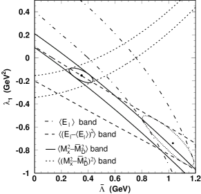
Figure 4: Bands in $\overline{\Lambda}-\lambda_{1}$ space found by CLEO in analyzing first and second moments of hadronic mass squared and lepton energy. The intersections of the two moments for each set determines the two parameters. The one standard deviation error ellipses are shown.

The two curves are shown in Fig. 4, that shows also the constraints derived from a similar analysis of the experimental moments of the lepton spectrum. It can be seen that the two sets of constraints do not intersect at a common point as they should. These data are still preliminary and we cannot draw definite conclusions from them. However until this discrepancy is resolved, this is yet another reason not to use an average value for $V_{cb}$ based on the inclusive and exclusive determinations.

3.3 The determination of $|V_{ub}|$ from exclusive charmless semileptonic decays

Unfortunately, in the case of $|V_{ub}|$ HQET does not help to normalize the relevant form factors. A variety of calculations of such form factors exist, based on lattice gauge theory [55], light cone sum rules (LCSR) [56], and quark models [57]. The CLEO collaboration has reported the first convincing evidence for the decays $B\rightarrow\rho\ell\overline{\nu}$ and $B\rightarrow\pi\ell\overline{\nu}$ [58]. CLEO has recently reported a measurement of the decay $B\rightarrow\rho\ell\overline{\nu}$ with a different technique and a bigger data sample [59]. They have used several different models to extract the value of $|V_{ub}|$. Their results are summarized in Table 4.

Table 4: Values of $|V_{ub}|$ using $B\rightarrow\rho\ell\overline{\nu}$ and some theoretical models. The $|V_{ub}|$ data include the results of a recent CLEO analysis [59] and a previous CLEO result on exclusive charmless semileptonic decays [60]. The average $|V_{ub}|$ includes an additional contribution representative of the theoretical uncertainty in the measurement.

Model	$|V_{ub}|$ ($\times 10^{-3}$)
UKQCD [55]	$3.32\pm 0.14^{+0.21}_{-0.26}$
LCSR [56]	$3.45\pm 0.15^{+0.22}_{-0.31}$
ISGW2 [57]	$3.24\pm 0.14^{+0.22}_{-0.29}$
Beyer-Melikhov [61]	$3.32\pm 0.15^{+0.21}_{-0.30}$
Wise/Ligeti [63]	$2.92\pm 0.13^{+0.19}_{-0.26}$
Average	$3.25\pm 0.14^{+0.21}_{-0.29}\pm 0.55$

The first three calculations are based on quark models and their uncertainties are guessed to be in the 25-50% range in the rate, corresponding to a 12.5-25% uncertainty for $|V_{ub}|$. The other approaches, light cone sum rules and lattice QCD, estimate their errors in the range of 30%, leading to a 15% error in $|V_{ub}|$. We can conclude that the average value of $|V_{ub}|$ extracted with this method is $|V_{ub}|=(3.25\pm 0.14^{+0.21}_{-0.31}\pm 0.5)\times 10^{-3}$. This corresponds to a value of $|V_{ub}/V_{cb}|=0.085\pm 0.023$. The statistical and systematic errors have been added in quadrature and the theoretical error has been added linearly to be conservative. Note that the theoretical error is somewhat arbitrary, as the spread between the models considered does not necessarily represent the uncertainty in $\Gamma_{u}^{th}$ nor may it properly reflect the effect of the lepton momentum cut of $>2.3$ GeV/c used in the analysis.

An alternative approach used by CLEO has been the investigation of the inclusive lepton spectrum beyond the kinematic endpoint of $B\rightarrow X_{c}\ell\overline{\nu}$ decays [64]. This method gave the first unambiguous evidence for charmless semileptonic decays, however its use to extract $|V_{ub}|$ is plagued by several theoretical uncertainties. In addition to the errors discussed above, there is the additional problem that very few models can be used to relate $\Gamma_{u}({\rm endpoint})$ with $\Gamma_{u}$. In fact, most of the models discussed above study only final states like $\rho\ell\overline{\nu}$ and $\pi\ell\overline{\nu}$, whereas it is likely that $\Gamma_{u}$ is composed of several different hadronic final states. The Operator Product Expansion (OPE) cannot give reliable predictions either, because when the momentum region considered is of the order of $\Lambda_{QCD}$ an infinite series of terms in this expansion may be relevant. Nonetheless the model dependent value extracted from these data has a central value of $|V_{ub}/V_{cb}|$=0.079 [65], very close to the exclusive result.

Recently, interest has been stirred by a new approach [66] to the extraction of $|V_{ub}|$ based on the OPE approach. The idea is that if the semileptonic width $\Gamma_{u}$ is extracted by integrating over the hadronic mass $X_{u}$ recoiling against the lepton neutrino pair in a sufficiently large region of phase space, the relationship between $|V_{ub}|$ and the measured value of the charmless semileptonic branching fraction can be reliably predicted. All the LEP experiments but OPAL attempted to use this technique to determine $|V_{ub}|$. An example of the lepton spectrum obtained by cutting on the measured $X_{u}<1.5$ GeV is shown in Fig. 5. Note that the claimed $|V_{ub}|$ signal is accompanied by a dominant $b\rightarrow c$ background. The three experiments combine their analyses and quote $|V_{ub}|=(4.05^{+0.39}_{-0.46}(stat+det)^{+0.43}_{-0.51}(b\rightarrow c)^{+0.23}_{-0.27}(b\rightarrow u)\pm 0.02(\tau_{b})\pm 0.16(HQE)\times 10^{-3}$ [67]. These results raise several concerns. First of all the small error on the $b\rightarrow c$ background component is not adequately justified. It implies a knowledge of the $b\rightarrow c$ background to better than 1%. Moreover the validity of the theoretical input applies only if the full phase space for the $b\rightarrow u\ell\overline{\nu}$ is measured. Even if the mass cut $M_{X}<1.5$ GeV should include most of the $\Gamma_{u}$ width, the complex set of event selection criteria applied may bias the phase space and make the errors in the $|V_{ub}|$ determination bigger than expected [68].

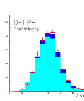
Figure 5: The lepton energy distribution in the $B$ rest frame from DELPHI. The data have been enriched in $b\to u$ events, and the mass of the recoiling hadronic system is required to be below 1.6 GeV. The points indicate data, the light shaded region, the fitted background and the dark shaded region, the fitted $b\to u\ell\nu$ signal.

Much work needs to be done to achieve a precise measurement of $|V_{ub}|$. This is a quite important element of our strategy to pin down the CKM sector of the Standard Model. On the theoretical side, large efforts are put in developing more reliable methods to determine the heavy to light form factors. A combination of several methods [69], all with a limited range of applicability, seem to be the strategy more likely to succeed. For instance, lattice QCD can provide reliable estimates of the form factors at large momentum transfer [78], where the discretization errors are under control. HQET predicts a relationship between semileptonic $D$ decays and semileptonic $B$ decays. To check these predictions and apply them to $|V_{ub}|$ estimates, large data sample with reconstructed neutrino momentum are necessary. For now, I use the $\rho\ell\overline{\nu}$ result as the best estimate of $|V_{ub}/V_{cb}|$. I take $|V_{ub}/V_{cb}|=0.085\pm 0.023$.

3.4 The present knowledge of the CKM parameters

In addition to the measurement of $|V_{ub}/V_{cb}|$, other experimental constraints can be used to check the $bd$ unitarity triangle.

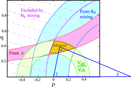
Figure 6: The CKM triangle shown in the $\rho-\eta$ plane. The shaded regions show $\pm 1\sigma$ contours given by $|V_{ub}/V_{cb}|$, neutral $B$ mixing, and CP violation in $K_{L}^{o}$ decay ($\epsilon$) [79]. The dashed region is excluded by $B_{s}$ mixing limits. The allowed region is defined by the overlap of the 3 permitted areas, and is where the apex of the CKM triangle sits.

An important input is the $\epsilon$ parameter describing $CP$ violation effects in $K$ decays [70]. Note that the $\epsilon$ parameter is the only constraint that forces $\eta$ to be positive. It is related to $\eta$ and $\rho$ through the relationship:

$$\eta\left[(1-\rho)A^{2}(1.4\pm 0.2)+0.35\right]A^{2}{B_{K}\over 0.75}=\\ (0.30\pm 0.06),$$

where the errors arise mostly from uncertainties on $|V_{cb}|$ and $B_{K}$. Recall that $A$ is one of the Wolfenstein parameters:

$$A=V_{cb}/\lambda^{2},\\ |\lambda|=|V_{us}|=0.220\pm 0.002.$$ (27)

$B_{K}$ is taken as 0.75$\pm$0.15 according to Buras [71]. Also the parameter $Re(\epsilon^{\prime}/\epsilon)$, recently measured with increased accuracy by KTeV [72] and NA48 [73] can be used. Several phenomenological calculations give $\eta$ as positive [74]. Note that a recent lattice calculation [75], using a novel algorithm involving domain wall fermions (DWF), obtains for the parameter $Re(\epsilon^{\prime}_{DWF}/\epsilon_{exp})$, a negative value of $-(3.3\pm 0.3_{stat}\pm 1.6_{sys})\times 10^{-2}\eta$, where $\eta$ is the CP violation parameter in the Wolfenstein parameterization of the CKM matrix. This result is quite recent and needs further studies [76], but it may imply a constraint in the $\rho-\eta$ plane not overlapping with the others and implies a violation of the Standard Model.

Finally neutral $B$ meson oscillations provide additional constraints, semicircles in the $\rho-\eta$ plane centered at $(\rho,\eta)=(1,0)$. The neutral $B_{d}$ oscillations are measured rather well [77]. The world average, including data from LEP, CDF, and SLD, gives $\Delta M_{d}=0.481\pm 0.017{\rm ps}^{-1}$. Only lower limits exist for $\Delta M_{s}$. The LEP average is 9.6 ps^-1, dominated by the 1998 ALEPH inclusive lepton analysis corresponding to a 95% C.L. lower limit of 9.5 ps^-1. The world average presented at Tampere is 12.4 ps^-1, whereas the most recent preliminary world average is 14.3 ps^-1. I will take as the world average the value of 12.4 ps^-1, because I believe that a preliminary value that is so much bigger than any individual measurement needs further scrutiny.

The constraints on $\rho$ versus $\eta$ from the $|V_{ub}/V_{cb}|$ determination, $\epsilon$ and $B$ mixing are shown in Fig. 6. The bands represent $\pm 1\sigma$ errors, for the measurements and a 95% confidence level upper limit on $B_{s}$ mixing. The width of the $B_{d}$ mixing band is caused mainly by the uncertainty on $f_{B}$, taken here as $240>f_{B}>160$ MeV.

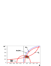
Figure 7: The allowed region for $\overline{\rho}$ and $\overline{\eta}$ according to Ref. [80]. The contours at 68 $\%$ and 95 $\%$ are shown. The full lines correspond to the central values of the constraints given by the measurements of $\frac{\left|V_{ub}\right|}{\left|V_{cb}\right|}$, $\epsilon$ and $\Delta m_{d}$. The dotted curve corresponds to the 95 $\%$ C.L. upper limit obtained from the experimental limit on $\Delta m_{s}$. The variables $\overline{\rho}$ and $\overline{\eta}$ are defined as $\overline{\rho}\equiv\rho(1-\lambda^{2})$ and $\overline{\eta}\equiv\eta(1-\lambda^{2})$.

Some authors have taken the data discussed above as the input of a global fit that is supposed to generate confidence level contours defined the Standard Model allowed region in the $\rho-\eta$ plane. Fig. 7 shows a recent example of such an analysis [80]. The big problem in works of this nature is how to combine in a reliable fashion results often dominated by theoretical uncertainties. Theoretical errors are often educated guesses [51] and thus not easily amenable to a rigorous statistical analysis. The relevance of the small contour that defines the Standard Model allowed region in this plot is questionable. For example, it will be very hard to attribute to a Standard Model failure any discrepancy between these results and new data coming from the next generation $b$ experiments that will be discussed later.

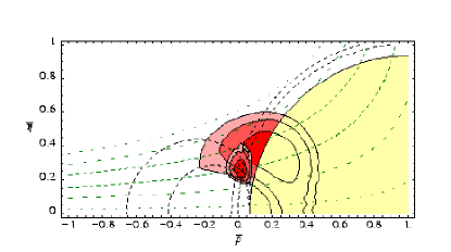
Figure 8: Fit 1 (smaller region) from Ref. [81]: prediction for $\rho$ and $\eta$ using the quark mass constraints from Eq. 29 and  29. Fit. 2 (larger region) corresponds to a SM fit using $|V_{ub}/V_{cb}|$, $\Delta m_{s}$, $\Delta m_{d}$ but not $\epsilon$. For both fits the countours are 68, 95 and 99 % C.L. respectively. The variables $\overline{\rho}$ and $\overline{\eta}$ are defined as $\overline{\rho}\equiv\rho(1-\lambda^{2})$ and $\overline{\eta}\equiv\eta(1-\lambda^{2})$.

There is one interesting idea that was proposed originally by H. Fritzsch [82] and is explored in several recent papers. Its starting point is the observation that both the quark masses and the quark mixing follow specific hierarchies. Perhaps these patterns contain a clue that can lead us to the more complete theory that we are so eagerly pursuing. In particular quark mass textures, i.e. specific patterns of zeros in quark mass matrices, that are motivated by attempts to understand the origing of flavour assuming a spontaneously broken symmetry, predict relationship between quark masses and quark mixing parameters. For example, Barbieri, Hall and Romanino [81] explored the constraints in the $\rho-\eta$ plane produced by the relationships:

$$\left|\frac{V_{ub}}{V_{cb}}\right|=\left(\frac{m_{u}}{m_{c}}\right)^{1/2}$$ (28)

$$\left|\frac{V_{td}}{V_{ts}}\right|=\left(\frac{m_{d}}{m_{s}}\right)^{1/2}$$ (29)

Fig. 8 shows the results from their analysis. Also in this case the contour plots should be taken with some reservations. It should be noted that their results are consistent with a Standard Model fit performed with the same technique as Roudeau et al.. The consistency is modest. This analysis illustrates another handle that we may use in the future more effectively to reach a more complete understanding of the mystery of flavour.

4 Rare $b$ Decays

“Rare” $b$ decays encompass a large class of decay modes, with branching fractions not necessarily exceedingly small, where a suppression mechanism reduces the rate compared to the dominant “tree diagram.” Fig. 9 shows the Feynman diagrams for the various decay processes considered. Fig 9 (a) shows a tree amplitude that is associated with $b\rightarrow u$ CKM suppressed decays.

$B^{0}-\bar{B^{0}}$ mixing occurs via a “box” diagram with virtual $W$ bosons and $t$ quarks inside the box [Figure 9(b)]. The box diagram gives rise to large fractions of mixed events: 17% for $B^{0}$ and 50% for $B_{s}$ mesons.

Flavor-changing neutral currents lead to the transitions $b\to s$ and $b\to d$. These can be described in the Standard Model by one-loop diagrams, known as “penguin” diagrams, where a $W^{-}$ is emitted and reabsorbed. The first such process to be observed was $b\to s\gamma$, described by the diagram in Figure 9(c), where the $\gamma$ can be radiated from any charged particle line. Another process which is important in rare $b$ decays is $b\to sg$, where $g$ designates a gluon radiated from a quark line [Figure 9(d)]. A third example of such processes is the transition $b\to s\ell^{+}\ell^{-}$ which can occur through the diagrams shown in Figures 9(e) and 9(f). We consider the loop processes shown in Figures 9 (c)-(f) to be among the most interesting and important rare $b$ decays.

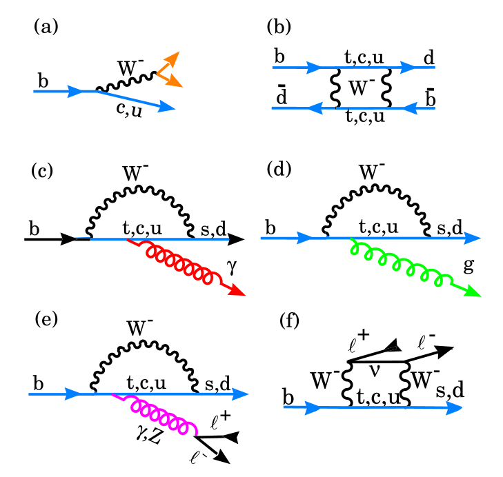
Figure 9: Feynman Diagrams for $b$ Decays

4.1 The decays $b\rightarrow s\gamma$ and $b\rightarrow s\ell^{+}\ell^{-}$

There are several reasons why the study of rare $b$ decays is very important. First of all, the suppression involved in loop diagrams makes it possible for these Standard Model processes to interfere with decay diagrams mediated by exotic mechanisms due to ‘beyond Standard Model’ interactions. In addition, loop diagrams and CKM suppression can affect our ability of measuring CP violation asymmetries.

CLEO has recently reported an updated value of this branching fraction, ${\cal B}(b\rightarrow s\gamma)=(3.15\pm 0.35\pm 0.32\pm 0.26)\times 10^{-4}$ [83], where the first uncertainty is statistical, the second is systematic and the third accounts for model dependence. ALEPH measured ${\cal B}(b\rightarrow s\gamma)=(3.11\pm 0.8\pm 0.72\pm 0.26)\times 10^{-4}$ [84], where the first error is statistical and the second is systematic, providing a nice confirmation of the CLEO result. In parallel a new theoretical estimate of the Standard Model prediction with a full next-to-leading-order-log calculation [85] has been performed, giving a predicted ${\cal B}(b\rightarrow s\gamma)=(3.28\pm 0.33)\times 10^{-4}$, in excellent agreement with the measured values.

The decay $b\rightarrow s\gamma$ was the first inclusive rare $b$ decay to be measured [86] and stirred a lot of theretical interest. It is a powerful constraint of theories “beyond the Standard Model.” For example, Masiero [87] identifies this process as “the most relevant place in flavor changing neutral current $B$ physics to constrain SUSY, at least before the advent of $B$ factories.”

The Standard Model predicts no CP asymmetry in $b\rightarrow s\gamma$. However recent theoretical work [62] suggested that non-Standard Model physics may induce a significant CP aysmmetry. Thus a search for CP asymmetry has been performed by CLEO. A preliminary results of ${\cal A}=(0.16\pm 0.14\pm 0.05)\times(1.0\pm 0.04)$ has been reported by CLEO [83]. The first number is the central value, followed by the statistical error and an additive systematic error. The multiplicative error is related to the uncertainty in the mistagging rate correction. From this result a 90% C.L. limit on the CP asymmetry ${\cal A}$ of $-0.09<{\cal A}<0.42$ is derived. These results are based on $\approx 3.1\ {\rm fb}^{-1}$ of data.

Another related decay mode that is quite important in constraining new physics is the decay $b\rightarrow s\ell^{+}\ell^{-}$ and the related exclusive channels $B\rightarrow K^{(\star)}\ell^{+}\ell^{-}$. These processes have been studied both at CLEO and at CDF and D0. Table 5 summarizes the searches for these decays.

Table 5: Searches for $b\rightarrow\ell^{+}\ell^{-}$ decays compared with Standard Model theoretical predictions [88].

$b$ decay	90% C.L.	Group	Prediction
mode	$\times 10^{-5}$		$(\times 10^{-6})$
$s\mu^{+}\mu^{-}$	$32$	D0 [89]	$(8\pm 2)$
	5.7	CLEO [90]
$K^{\star o}\mu^{+}\mu^{-}$	0.4	CDF [91]	$2.9$
	$1.1$	CLEO [92]
$K^{\star o}e^{+}e^{-}$	$1.3$	CLEO [92]	$5.6$
$K^{-}\mu^{+}\mu^{-}$	$0.83$	CLEO [92]	$0.6$
	$0.52$	CDF [91]
$K^{-}e^{+}e^{-}$	$1.1$	CLEO [92]	$0.6$

4.2 Rare Hadronic $b$ Decays

Fig. 9 includes the dominant diagrams mediating rare $B$ hadronic decays. The interplay between penguin and loop diagrams may affect our ability of measuring CP asymmetries in two different ways. On one hand, loops and CKM suppressed diagrams can lead to final states accessible to both $B$ and $\overline{B}$ decays, making it possible to measure interference effects without neutral $B$ mixing. On the other hand, the interplay between these two processes can cloud the relationship between measured $CP$ asymmetries and the CKM phase when mixing induced CP violation is looked for. A classical example of this effect is the decay $B^{o}\rightarrow\pi^{+}\pi^{-}$. The main Standard Model diagrams contributing to this decay process are shown in Fig. 9 (a) and (d). If the $b\rightarrow u$ diagram is dominant, the angle $\alpha$ can be extracted from the measurement of the asymmetry in the decay $B^{o}\rightarrow\pi^{+}\pi^{-}$. On the other hand, if these two diagrams have comparable amplitude, the extraction of $\alpha$ from this decay channel is going to be a much more difficult task.

CLEO has studied several decays that can lead to a more precise understanding of the interplay between penguin diagrams and $b\rightarrow u$ diagrams in $B$ meson decays. The analysis technique used has been extensively refined in order to make the best use of the limited statistics presently available. In most of the decay channels of interest, the dominant source of background are continuum events; the fundamental difference between $e^{+}e^{-}\rightarrow q\overline{q}$ and $B$ decays is the shape of the underlying event. The latter decays tend to produce a more ‘spherical’ distribution of particles whereas continuum events tend to be more ‘jet-like’, with most of the particle emitted into two narrow back to back ‘jets’. This property can be translated into several different shape variables. CLEO constructs a Fisher discriminant ${\cal F}=\Sigma_{i}\alpha_{i}y_{i}$, a linear combination of several variables $y_{i}$. The variables used are $|\cos{\theta_{cand}}|$, the cosine of the angle between the candidate $B$ sphericity axis and the beam axis, the ratio of Fox-Wolfram moments $R_{2}=H_{2}/H_{0}$, and nine variables that measure the scalar sum of the momenta of the tracks and showers from the rest of the event in 9 angular bins, each of 10^∘, around the candidate sphericity axis. The coefficients $\alpha_{i}$ have been chosen to optimize the separation between signal and background Monte Carlo samples [93]. In addition, several kinematical constraints allow a more precise determination of the final state. First of all they consider the energy difference $\Delta E=E_{cand}-E_{B}$, where $E_{cand}$ is the reconstructed candidate mass and $E_{B}$ is the known beam energy ($\Delta E=0$ for signal events) and the beam constrained mass $M_{B}$ calculated from $M_{B}^{2}=E_{beam}^{2}-\left(\Sigma_{i}\vec{p}_{i}\right)^{2}$. In addition, the $B$ decay angle with respect to the beam axis has a $\sin^{2}(\theta_{B})$ angular distribution. Finally, to improve the separation between the final states $K\pi$ and $\pi\pi$ the specific energy loss in the drift chamber, $dE/dx$ is used.

CLEO uses a sophisticated unbinned maximum likelihood (ML) fit to optimize the precision of the signal yield obtained in the analysis, using $\Delta E$, $M_{B}$, ${\cal F}$, $|\cos{\theta_{B}}|$, and $dE/dx$ wherever applicable. In each of these fits the likelihood of the event is parameterized by the sum of probabilities for all the relevant signal and background hypotheses, with relevant weights determined by maximizing the likelihood function (${\cal L}$). The probability of a particular hypothesis is calculated as the product of the probability density functions for each of the input variables determined with high statistics Monte Carlo samples. The likelihood function is defined as:

$${\cal L}=\Pi_{k}\Sigma_{i}P^{i}_{k}(\Delta E,M_{B},{\cal F},dE/dx,\cos{\theta_{B}})\times f_{i}$$ (30)

where the index $k$ runs over the number of events, the index $i$ over the hypotheses considered, $P^{i}_{k}$ are the probabilities for different hypotheses obtained from Monte Carlo simulations of the signal and background channels considered and independent data samples, and $f_{i}$ are the fractional yields for hypothesis $i$, with the constraint:

$$\Sigma_{i}f_{i}=1$$ (31)

Further details about the likelihood fit can be found elsewhere [93]. The fits include all the decay channels having a similar topology. For example, in the final state including two charged hadrons, the final states considered were $K^{\pm}\pi^{\mp}$, $\pi^{+}\pi^{-}$ and $K^{+}K^{-}$.

Figure 10: Contours of the $-2\ln{\cal L}$ for the ML fit to $N_{K^{\pm}\pi^{\mp}}$ and $N_{\pi^{+}\pi^{-}}$, the $K^{\pm}\pi^{\mp}$ and $\pi^{+}\pi^{-}$ yields respectively.

Figure 11: Projections of $K\pi$ and $\pi\pi$ events onto $M$ and $\Delta E$ with cuts. Upper left: $M$ distribution of $K\pi$-like events; upper right: $M$ distribution of $\pi\pi$-like events. Lower left: $\Delta E$ distribution of events prior to $\pi\pi$ vs $K\pi$ vs $KK$ selection according to dE/dx; Lower right: $\Delta E$ distribution of events that are more likely to be $\pi\pi$ than $K\pi$ or $KK$ based on dE/dx. Overlays in the lower plots are the results of the likelihood fit scaled by the efficiency of the cuts used to project into these plots. Solid line: total fit; dashed: $K\pi$; dotted: $\pi\pi$; dot-dash: continuum background.

Fig. 10 shows contour plots of the ML fits for the signal yields in the $K^{\pm}\pi^{\mp}$ and $\pi^{+}\pi^{-}$ final states. The other channels included in the likelihood function have $f_{i}$ fixed to their most probable value extracted from the fit. It can be seen that there is a well defined signal for both the final states $K^{\pm}\pi^{\mp}$ and $\pi^{+}\pi^{-}$. The ratio between the most probable yields in the two channels shows that the $b\rightarrow u$ diagram is suppressed with respect to the penguin diagram in $B$ decays to two pseudoscalar mesons. Fig. 11 shows distributions in $M_{B}$ and $\Delta E$ for events after cuts on the Fisher discriminant and whichever of $M$ and $\Delta E$ is not being plotted, plus an exclusive classification into $K\pi$-like and $\pi\pi$-like candidates based on the most probable assignment with $dE/dx$ information. The likelihood fit, suitably scaled to account for the efficiencies of the additional cuts, is overlaid in the $\Delta E$ distributions to illustrate the separation between $K\pi$ and $\pi\pi$ events.

Table 6 summarizes the CLEO results for the $B\rightarrow K\pi,~{}\pi\pi,~{}KK$ final states. Unless explicitly stated, the preliminary results are based on 9.66 million $B\overline{B}$ pairs collected with the CLEO detector.

There is a consistent pattern of penguin dominance in $B$ decays into two charmless pseudoscalar mesons that makes the prospects of extracting the angle $\alpha$ from the study of the CP asymmetry in the $B\rightarrow\pi^{+}\pi^{-}$ mode less favorable than originally expected.

Table 6: Experimental results. Branching fractions (${\cal B}$) and 90% C.L. upper limits are given in units of $10^{-6}$.

Mode	${\cal B}$($10^{-6}$)	Signif.($\sigma$)
$\pi^{+}\pi^{-}$	$4.7^{+1.8}_{-1.5}\pm 0.6$	4.2
$\pi^{+}\pi^{0}$	$<12$	3.2
$K^{+}\pi^{-}$	$18.8^{+2.8}_{-2.6}\pm 1.3$	11.7
$K^{+}\pi^{0}$	$12.1^{+3.0+2.1}_{-2.8-1.4}$	6.1
$K^{0}\pi^{+}$	$18.2^{+4.6}_{-4.0}\pm 1.6$	7.6
$K^{0}\pi^{0}$	$14.8^{+5.9+2.4}_{-5.1-3.3}$	4.7
$K^{+}K^{-}$	$<2.0$	–
$K^{+}\overline{K}^{0}$	$<5.1$	1.1

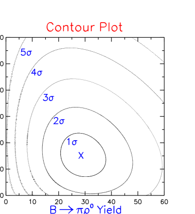
Figure 12: $n\sigma$ contours for the decays $B^{+}\rightarrow\rho^{0}\pi^{+}$ and $B^{+}\rightarrow\rho^{0}K^{+}$. The cross identifies the most probable values of the yields for these two channels.

Recent CLEO data suggest that final states involving a vector and a pseudoscalar meson offer a different picture. In fact, $B^{+}\rightarrow\pi^{+}\rho^{o}$ and $B\rightarrow\rho^{\pm}\pi^{\mp}$ [94] have been observed, while the penguin dominated final states $B^{+}\rightarrow K\rho$ and $B\rightarrow K^{\star}\pi$ have not. The analysis procedure is similar to the one adopted for the charmless pseudoscalar-pseudoscalar exclusive decays. In this quasi two-body case, there are three particles in the final state and some additional constraints are provided by the vector particle decay kinematics. The invariant mass of its decay products must be consistent with the vector meson mass. In addition, the vector meson is polarized, thus its helicity angle $\theta_{h}$ has a $\cos^{2}{\theta_{h}}$ distribution. The maximum likelihood fit includes $\pi\rho^{0}$ and $K\rho^{0}$ signal channels and continuum samples. The $n\sigma$ contour plot for this analysis is shown in Fig. 12 and gives solid evidence for a $B^{+}\rightarrow\pi^{+}\rho^{o}$ signal, while the $B^{+}\rightarrow K^{+}\rho^{o}$ channel appears to be suppressed. Table 7 shows the results for each decay mode investigated. For observations the final result is reported as a branching fraction central value, while for modes where the yield is not sufficiently significant the 90% confidence level upper limit is quoted. Also listed in the Table are theoretical estimates.

Table 7: Summary of CLEO results on charmless hadronic decays to a final state including a vector and a pseudoscalar meson compared with expectations from theoretical models.

Decay mode	$\mbox{${\cal B}$}(10^{-6})$	Theory ${\cal B}$ ($10^{-6}$)	References
$B^{+}\rightarrow\omega\pi^{+}$	$11.3^{+3.3}_{-2.9}\pm{1.5}$	$0.6-11$	[95, 96, 102, 97, 98, 99, 100, 101]
$B^{0}\rightarrow\omega\pi^{0}$	$<5.8$	$0.01-12$	[95, 96, 97, 98, 99, 100, 101]
$B^{+}\rightarrow\omega K^{+}$	$<8.0$	$0.2-13$	[95, 96, 102, 97, 98, 99, 100, 101]
$B^{0}\rightarrow\omega K^{0}$	$<21$	$0.02-10$	[95, 96, 97, 98, 99, 100, 101]
$B^{+}\rightarrow\omega h^{+}$	$14.3^{+3.6}_{-3.2}\pm 2.1$
$B^{+}\rightarrow\omega\rho^{+}$	$<47$	$7-28$	[95, 96, 103, 99, 100, 101]
$B^{0}\rightarrow\omega\rho^{0}$	$<11$	$0.005-0.4$	[95, 99, 100, 101]
$B^{+}\rightarrow\omega K^{*+}$	$<52$	$0.9-15$	[95, 96, 103, 99, 100, 101]
$B^{0}\rightarrow\omega K^{*0}$	$<19$	$0.3-12$	[95, 96, 99, 100, 101]
$B^{+}\rightarrow\rho^{0}\pi^{+}$	$15^{+5}_{-5}\pm 4$	$0.4-8$	[95, 104, 96, 102, 97, 98, 99, 100, 101]
$B^{0}\rightarrow\rho^{-}\pi^{+}$	$35^{+11}_{-10}\pm 5$	$26-52$	[95, 104, 96, 97, 98, 99, 100, 101]
$B^{0}\rightarrow\rho^{0}\pi^{0}$	$<5.1$	$0.9-2.3$	[95, 104, 97, 98, 99, 100, 101]
$B^{+}\rightarrow\rho^{0}K^{+}$	$<22$	$0.1-1.7$	[105, 95, 96, 102, 97, 98, 99, 100, 101]
$B^{0}\rightarrow\rho^{-}K^{+}$	$<25$	$0.2-2.5$	[105, 95, 96, 97, 98, 99, 100, 101]
$B^{0}\rightarrow\rho^{0}K^{0}$	$<27$	$0.04-1.7$	[105, 95, 96, 97, 98, 99, 100, 101]
$B^{+}\rightarrow K^{*0}\pi^{+}$	$<27$	$4-12$	[105, 95, 107, 97, 98, 99, 100, 101]
$B^{0}\rightarrow K^{*+}\pi^{-}$	$22^{+8\;+4}_{-6\;-5}$	$1.2-19$	[105, 95, 96, 97, 98, 99, 100, 101]
$B^{0}\rightarrow K^{*0}\pi^{0}$	$<4.2$	$1.1-5$	[105, 95, 96, 97, 98, 99, 100, 101]
$B^{0}\rightarrow K^{*+}K^{-}$	$<6$
$B^{+}\rightarrow K^{*0}K^{+}$	$<12$	$0.2-1$	[95, 102, 97, 98, 100, 101]
$B^{+}\rightarrow\phi\pi^{+}$	$<4.0$	$0.001-0.4$	[106, 96, 107, 102, 97, 98, 99, 100, 101]
$B^{0}\rightarrow\phi\pi^{0}$	$<5.4$	$0.0004-0.2$	[106, 96, 107, 97, 98, 99, 100, 101]
$B^{+}\rightarrow\phi K^{+}$	$<5.9$	$0.3-18$	[105, 95, 96, 107, 108, 102, 97, 98, 99, 100, 101]
$B^{0}\rightarrow\phi K^{0}$	$<28$	$0.3-18$	[105, 95, 96, 107, 108, 97, 98, 99, 100, 101]

The stronger $b\rightarrow u$ component in vector to pseudoscalar final states suggests that an approach, proposed by Snyder and Quinn [109] can lead to a precise measurement of the angle $\alpha$. The interference between Tree and Penguin diagrams can be measured through the time dependent CP violating effects in the decays $B^{o}\to\rho\pi\to\pi^{+}\pi^{-}\pi^{o}$. Since the $\rho$ is spin-1, the $\pi$ spin-0 and the initial $B$ also spinless, the $\rho$ is fully polarized in the (1,0) configuration, so the helicity angle has a $\cos^{2}{\theta}$ distribution. This causes the periphery of the Dalitz plot to be heavily populated, especially the corners. A sample Dalitz plot is shown in Fig. 13.

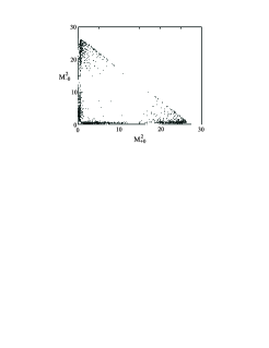
Figure 13: The Dalitz plot for $B^{o}\to\rho\pi\to\pi^{+}\pi^{-}\pi^{o}$ from Snyder and Quinn.

Snyder and Quinn performed an idealized analysis that showed that a background free 1000 or 2000 flavor tagged event samples is sufficient to measure $\alpha$.

These charmless hadronic decays can, in principle, provide also some information on the phase $\gamma$, conventionally defined as the argument of $V_{ub}$. This phase can cause asymmetries in decay rates to charge conjugate pairs. CLEO has taken a first look at possible evidence for these rate asymmetries. No positive signal has been seen and the present sensitivity is shown in Table 8 summarizing their preliminary results.

Table 8: ${{\cal A}_{\rm CP}}$ measurements in five charmless $B$ decay modes. CLEO 1999 Preliminary.

Mode	${\cal S}$	${\overline{\mbox{${\cal S}$}}}$	${{\cal A}_{\rm CP}}$	90% CL
$K\pi^{0}$	$16.8\pm 7.5$	$28.9\pm 7.5$	$-0.27\pm 0.23\pm 0.05$	$[-0.70,0.16]$
$K^{0}_{S}\pi$	$14.5\pm 4.4$	$10.2\pm 4.0$	$0.17\pm 0.24\pm 0.05$	$[-0.27,0.61]$
$K\pi$	$38.6_{-8.1}^{+9.0}$	$41.6_{-8.0}^{+8.9}$	$-0.04\pm 0.16\pm 0.05$	$[-0.35,0.27]$
$\mbox{$\eta^{\prime}$}K$	$51.7\pm 9.2$	$48.7\pm 8.9$	$0.03\pm 0.12\pm 0.05$	$[-0.22,0.28]$
$\omega\pi$	${{9.4}^{+4.9}_{-4.0}}$	${{19.1}^{+6.8}_{-5.9}}$	$-0.34\pm 0.25\pm 0.05$	$[-0.80,0.12]$

Table 9: Summary of CLEO results for $B$ branching fractions to charmless final states involving an $\eta$ or $\eta^{\prime}$ mesons. The second column gives recent preliminary result [110], unless otherwise stated. The central value followed by statistical and systematic error is given if significantly above zero, otherwise as a 90% confidence level upper limit is quoted. Estimates from various theoretical sources are shown for comparison.

Decay mode	$\mbox{${\cal B}$}(10^{-6})$	Signif. ($\sigma$)	Theory ${\cal B}$($10^{-6}$)
$B^{+}\rightarrow\mbox{$\mbox{$\eta^{\prime}$}K^{+}$}$	$80^{+10}_{-9}\pm 8$	16.8	7 – 65 [95, 97]
$B^{0}\rightarrow\mbox{$\mbox{$\eta^{\prime}$}K^{0}$}$	$88^{+18}_{-16}\pm 9$	11.7	9 – 59 [95, 97]
$B^{+}\rightarrow\mbox{$\mbox{$\eta^{\prime}$}\pi^{+}$}$	$<11$	$0.2$	1 – 23 [95, 97]
$B^{0}\rightarrow\mbox{$\mbox{$\eta^{\prime}$}\mbox{$\pi^{0}$}$}$[111]	$<11$	–	0.1 – 14 [95, 97]
$B^{+}\rightarrow\mbox{$\mbox{$\eta^{\prime}$}K^{*+}$}$[112]	$<87$	1.2	0.1 – 3.7 [95, 97]
$B^{0}\rightarrow\mbox{$\mbox{$\eta^{\prime}$}K^{*0}$}$[112]	$<20$	1.0	0.1 – 8.0 [95, 97]
$B^{+}\rightarrow\mbox{$\mbox{$\eta^{\prime}$}\rho^{+}$}$ [111]	$<47$	–	3 – 24 [95, 97]
$B^{0}\rightarrow\mbox{$\mbox{$\eta^{\prime}$}\rho^{0}$}$ [111]	$<23$	–	0.1 – 11 [95, 97]
$B^{+}\rightarrow\mbox{$\eta K^{+}$}$	$<7.1$	1.0	0.2 – 5.0 [95, 97]
$B^{0}\rightarrow\mbox{$\eta K^{0}$}$	$<9.5$	–	0.1 – 3.0 [95, 96, 97]
$B^{+}\rightarrow\mbox{$\eta\pi^{+}$}$	$<6.0$	0.6	1.9 – 7.4 [95, 96, 97]
$B^{0}\rightarrow\mbox{$\eta\mbox{$\pi^{0}$}$}$	$<3.1$	–	0.2 – 4.3 [95, 97]
$B^{+}\rightarrow\mbox{$\eta K^{*+}$}$	$27.3^{+9.6}_{-8.2}\pm 5.0$	4.8	0.2 – 8.2 [95, 97]
$B^{0}\rightarrow\mbox{$\eta K^{*0}$}$	$13.8^{+5.5}_{-4.4}\pm 1.7$	5.1	0.1 – 8.9 [95, 96, 97]
$B^{+}\rightarrow\mbox{$\eta\rho^{+}$}$	$<16$	1.3	4 – 17 [95, 96, 97]
$B^{0}\rightarrow\mbox{$\eta\rho^{0}$}$	$<11$	1.3	0.1 – 6.5 [95, 96, 97]

The branching fractions themselves can be used to constraint the angle $\gamma$. Several approaches have been pursued and they are more or less model dependent [113]. Atwood and Soni performed a general analysis of $B$ decays involving 10 $B$ decay modes to pseudoscalar final states [114] for the charged and neutral $B$ mesons respectively. Their analysis has been recently updated to include the results discussed in this paper. Conjugate pairs have been taken together since the experimental data are not yet sensitive to CP violation effects. Rescattering effects are attributed to a single complex parameter $\kappa$. This analysis determines 8 parameters, tree amplitude $t$, color suppressed amplitude $\hat{t}$, penguin amplitude $p$, electroweak penguin amplitude $e$, real $\kappa=\kappa_{R}$, imaginary $\kappa=\kappa_{I}$, and the CKM parameters $\rho$ and $\eta$. A self-consistent solution is sought for using a $\chi^{2}$ minimization. Several fits are performed using different simplifying assumptions. The best fits are obtained assuming that electroweak penguin and rescattering effects are negligible. In this case the authors obtain a value of $\gamma=92\pm 20$ degrees.

Recently Hou, Smith and Wüerthwein [115] have performed a similar analysis, including final states composed by two pseudoscalar mesons and a vector and a pseudoscalar meson. They perform a fit with the same procedure as one of the fits by Atwood and Soni, with the restrictive assumption of factorization. They obtain $\gamma=114^{+25}_{-21}$ degrees. The $VP$ final states have been studied with flavor SU(3) by Gronau and Rosner [116] and they found that several processes are consistent with $\cos{\gamma}<0$. These results are preliminary. These studies illustrate the increasing interest in these decays to measure fundamental Standard Model parameters. However to reach definite conclusion, a deeper understanding of hadronic physics must be achieved.

The CLEO study of $B$ decays to final states including two charmless hadrons has presented some other interesting surprises. A large branching ratio has been discovered for final states including a $\eta^{\prime}$ meson. The analysis technique in this case is essentially the same as the one discussed above. The $\eta^{\prime}$ is reconstructed both in its $\eta\pi^{+}\pi^{-}$ and $\rho\gamma$ decay channels. The results for different decay modes including $\eta$ and $\eta^{\prime}$ are summarized in Table 9. The most notable feature is the astonishing large rate for the $\eta^{\prime}K$ final state. While several theoretical interpretations have been proposed to explain this enhancement [117], a very plausible explanation still points to a dominance of penguin effects.

5 The lesson from charm

Charm is a unique probe of the Standard Model in the up quark sector, thus providing a window of opportunity to discover new physics complementary to that attainable from the down-quark sector. Due to the effectiveness of the GIM mechanism, short distance contribution to rare charm processes are extremely small. Thus very often long range effects, for which reliable calculations are rarely available, dominate the rates. On the other hand the fact that the Standard Model predictions are so small for flavor changing neutral currents in the charm sector provides a unique opportunity to discover new physics in charm rare decays, $D^{o}\bar{D}^{o}$ mixing and CP violation in the decays of charmed mesons.

5.1 Rare and Forbidden decays of charmed mesons

Flavor changing neutral current (FCNC) decays of the $D$ meson include the processes $D^{o}\rightarrow\ell^{+}\ell^{-},\ \gamma\gamma$, and $D\rightarrow X_{u}\gamma,\ X_{u}\nu\overline{\nu},\ X_{u}\ell^{+}\ell^{-}$. They proceed via electromagnetic or weak penguin diagrams, with contributions from box diagrams in some cases. Calculations of short distance contributions to these decays are quite reliable [118], however the long range contribution estimates are plagued with hadronic uncertainties and are mentioned here to give an approximate upper limit of the size of these effects.

Table 10 summarizes some theoretical predictions together with the experimental upper limits coming from fixed target charm experiments, most notably E791 [119], and CLEO. Soon another fixed target experiment at Fermilab, FOCUS, should provide an improvement of about a factor of 10 [120]. These decays are usually classified into three categories:

• Flavor changing neutral current (FCNC) decays, such as $D^{o}\rightarrow\ell^{+}\ell^{-}$ and $D^{o}\rightarrow X\ell^{+}\ell^{-}$,

• Lepton family number violating (LFNV) such as $D^{+}\rightarrow h^{-}\mu^{\pm}e^{\mp})$,

• Lepton number violating (LNV) decays such as $D^{+}\rightarrow h^{-}\mu^{+}\mu^{+}$.

The first decays (FCNC) are rare, namely they are processes that can proceed via an internal quark loop in the Standard Model. The other two categories are strictly forbidden within the Standard Model. However they are are allowed in some of its extensions, such as extended technicolor [118]. The expected rates for class (1) decays are several orders of magnitude below the experimental sensitivity. However this may represent a window of opportunity to discover new physics.

Table 10: Measured experimental limits for various rare $D$ meson decays together with the Standard Model predictions for the branching fractions due to short (${\cal B}_{SD}$) and long distance contributions ((${\cal B}_{LD}$).

Decay Mode	Experimental limit (90 % C.L.)	${\cal B}_{SD}$)	(${\cal B}_{LD}$)
$D^{o}\rightarrow\mu^{+}\mu^{-}$	$4.1\times 10^{-6}$ [121]	$(1-20)\times 10^{-19}$	$<3\times 10^{-15}$
$D^{o}\rightarrow e^{+}e^{-}$	$6.2\times 10^{-6}$ [119] $(2.3-4.7)\times 10^{-24}$	–
$D^{o}\rightarrow\mu^{\pm}e^{\mp}$	$8.1\times 10^{-6}$ [119]	$0$	$0$
$D^{o}\rightarrow\gamma\gamma$	–	$10^{-16}$	$<10^{-9}$
$D\rightarrow X_{u}\gamma$		$1.4\times 10^{-7}$	–
$D^{o}\rightarrow\rho^{o}\gamma$	$2.4\times 10^{-4}$ [121]	–	$<2\times 10^{-5}$
$D^{o}\rightarrow\phi\gamma$	$1.9\times 10^{-4}$ [121]	–	$<10^{-4}$
$D^{+}\rightarrow\rho^{+}\gamma$			$2\times 10^{-4}$
$D^{o}\rightarrow X_{u}\ell^{+}\ell^{-}$		$4\times 10^{-9}$
$D^{o}\rightarrow\pi^{o}ee/\mu\mu$	$(4.5/2.6)\times 10^{-5}$ [121]
$D^{o}\rightarrow\overline{K}^{o}ee/\mu\mu$	$(1.1/2.6)\times 10^{-4}$ [121]		$<2\times 10^{-15}$
$D^{o}\rightarrow\rho^{o}ee/\mu\mu$	$1.0/2.3\times 10^{-4}$ [121]
$D^{+}\rightarrow\pi^{+}ee/\mu\mu$	$(5.2/1.5)\times 10^{-5}$ [119]	few$\times 10^{-10}$	$<10^{-8}$
$D^{+}\rightarrow K^{+}ee/\mu\mu$	$(20/4.4)\times 10^{-5}$ [119]	few$\times 10^{-10}$	$<10^{-8}$

5.2 CP Violation and $D^{o}\overline{D}^{o}$ Mixing

Another window of opportunity towards new physics discoveries is provided by the study of CP violation and flavour oscillations in charm decays. Both effects are expected to be highly suppressed. CP violation asymmetries are expected to be around $10^{-3}$ [122] in Cabibbo suppressed decay such as $D^{+}\rightarrow K^{-}K^{+}\pi^{+}$ and $D^{o}\rightarrow K^{-}K^{+}$. Recent preliminary results from Focus [120] based on 59% of their data have given ${\cal A}_{CP}=-0.004\pm 0.017$ for the decay mode $D^{+}\rightarrow K^{-}K^{+}\pi^{+}$ and ${\cal A}_{CP}=0.003\pm 0.039$ for $D^{o}\rightarrow K^{-}K^{+}$.

In the case of the $D^{o}$ the asymmetry may be a combination of direct CP asymmetry and indirect CP asymmetry mediated by mixing. The $D^{o}\overline{D}^{o}$ mixing parameter $\Delta M_{D}$ is affected by small distance contributions described by box diagrams via internal $d,\ s,\ b$ quarks and long distance contributions that are more difficult to evaluate. At any rate, the Standard Model expectations for $\Delta M_{D}$ are between $10^{-18}$ and $10^{-16}$ [118].

The probability that a $D^{o}$ oscillates into a $\overline{D}^{o}$ is generally expressed as:

$$I(t)\propto\left|\frac{q}{p}\right|^{2}e^{-\Gamma_{1}t}\left[1+e^{\Delta\Gamma t}+2e^{0.5\Delta\Gamma t}\cos{\Delta mt}\right]$$ (32)

where $\Delta m\equiv m_{1}-m_{2}$, $\Delta\Gamma=\Gamma_{1}-\Gamma_{2}$ and the subscripts 1 and 2 identify the two neutral $D$ meson mass eigenstates and the complex parameters $p$ and $q$ account for CP violation effects.

The parameter $r_{WS}$ for the decay $D^{o}\rightarrow K^{+}\pi^{-}$ can be expressed as:

$$r_{ws}\approx e^{-\Gamma t}\begin{array}[]{l}[r_{D}+r_{mix}\times\frac{\Gamma^{2}t^{2}}{2}+\\ \sqrt{2r_{mix}r_{D}}\cos{\Phi}\times\Gamma t]\end{array}$$ (33)

where the first term is the $DCSD$ contribution parameterized by the quantity $r_{D}$, the second is the one due to mixing and the last one is an interference term between mixing and $DCSD$. The latter term is set to zero for simplicity in some of the experimental estimates of $r_{mix}$, but this is not a legitimate assumption. Alternatively, we can parameterize $r_{ws}$ as:

$$r_{ws}=e^{-t}\begin{array}[]{l}[R_{D}+\sqrt{R_{D}}y^{\prime}t+\\ +\frac{1}{4}({x^{\prime}}^{2}+{y^{\prime}}^{2})t^{2}]\end{array}$$ (34)

where $R_{D}$ is the rate of the direct doubly-Cabibbo-suppressed decay $\overline{D}^{o}\rightarrow K^{+}\pi^{-}$, $x^{\prime}=x\cos{\delta}+y\sin{\delta}$ and $y^{\prime}=y\cos{\delta}-x\sin{\delta}$ and $x=\Delta M/\overline{\Gamma}$, $y=\Delta\Gamma/\overline{\Gamma}$. $\overline{\Gamma}$ represents the average lifetime and $\delta$ represents a strong phase between the doubly-Cabibbo-suppressed decay and the Cabibbo favored one. CLEO [123] has recently used the formulation in Eq. 34 to obtain a very precise measurement of the parameter $R_{D}=0.50^{+0.11}_{-0.12}\pm 0.08$. Their limit at 95 % C.L. are $(1/2){x^{\prime}}^{2}<0.05\%$ and $-5.9\%<y^{\prime}<0.3\%$. E791 has extracted the mixing parameter $r_{mix}$ [124] also from the semileptonic decay $D^{o}\rightarrow K\ell\nu$. This leads to a more straightforward determination because the $DCSD$ contribution is absent, obtaining $r_{mix}<0.50\%$ at 90% C.L. Thus the amplitudes that describe $D^{o}\overline{D}^{o}$ are still consistent with 0. Soon CLEO and FOCUS results based on semileptonic data will be available [120].

6 Outlook

The selected sample of flavour physics topics that I have discussed shows that there are several predictions of the Standard Model that we have yet to test thoroughly. In particular we must explore the phenomenology of CP violation in $b$ and $c$ decays, flavour oscillations in the $B_{s}$ system and study rare decays of beauty and charm. Our ability to challenge the Standard Model and to discover new physics will rely on two different areas where progress is needed. On one hand, we need to reach a new level of sophistication in our experimental study of these decays. On the other hand, we need to refine the theoretical inputs, to develop less model dependent predictions for a larger class of branching fractions and CP asymmetries.

Table 11: Required Measurements for $b$’s

Physics	Decay Mode	Hadron	$K\pi$	$\gamma$	Decay
Quantity		Trigger	sep	det	time $\sigma$
$\sin(2\alpha)$	$B^{o}\to\rho\pi\to\pi^{+}\pi^{-}\pi^{o}$	$\surd$	$\surd$	$\surd$
$\cos(2\alpha)$	$B^{o}\to\rho\pi\to\pi^{+}\pi^{-}\pi^{o}$	$\surd$	$\surd$	$\surd$
sign$(\sin(2\alpha))$	$B^{o}\to\rho\pi$ & $B^{o}\to\pi^{+}\pi^{-}$	$\surd$	$\surd$	$\surd$
$\sin(\gamma)$	$B_{s}\to D_{s}^{\pm}K^{\mp}$	$\surd$	$\surd$		$\surd$
$\sin(\gamma)$	$B^{-}\to\overline{D}^{0}K^{-}$	$\surd$	$\surd$
$\sin(\gamma)$	$B^{o}\to\pi^{+}\pi^{-}$ & $B_{s}\to K^{+}K^{-}$	$\surd$	$\surd$		$\surd$
$\sin(2\chi)$	$B_{s}\to J/\psi\eta^{\prime},$ $J/\psi\eta$			$\surd$	$\surd$
$\sin(2\beta)$	$B^{o}\to J/\psi K_{s}$
$\cos(2\beta)$	$B^{o}\to J/\psi K^{o}$, $K^{o}\to\pi\ell\nu$
$\cos(2\beta)$	$B^{o}\to J/\psi K^{*o}$ & $B_{s}\to J/\psi\phi$				$\surd$
$x_{s}$	$B_{s}\to D_{s}^{+}\pi^{-}$	$\surd$			$\surd$
$\Delta\Gamma$ for $B_{s}$	$B_{s}\to J/\psi\eta^{\prime}$, $D_{s}^{+}\pi^{-}$, $K^{+}K^{-}$	$\surd$	$\surd$	$\surd$	$\surd$

I will focus my discussion on the experimental techniques most suitable for a thorough investigation of beauty and charm decays. Table 11 summarizes the measurements that need to be done in beauty physics in order to overconstrain the CKM matrix. The first measurements of some of these quantities will be performed by the several new or upgraded experiments pursuing $b$ physics in the next few years. In particular the $e^{+}e^{-}$ experiments, CLEO, BaBar and Belle should see CP violation in 2000. CLEO is sensitive to direct CP violation in rare decays. BaBar and Belle should also see CP violation in $B\rightarrow\psi K_{s}$, where CDF has already seen a hint [125] . CDF and D0 are scheduled to turn on in 2001 and are both planning to pursue some of these measurements. HERA-B should also turn on in this time scale. Moreover ATLAS and CMS are planning to study CP violation in $B\rightarrow\psi K_{s}$ when LHC turns on.

None of these experiments is capable of completing the physics program summarized in Table 11. The $e^{+}e^{-}$ facilities are limited in statistical accuracy for several measurements due to the low cross section for $B\overline{B}$ production. Furthermore, they cannot address $B_{s}$ physics. On the other hand, the current, upgraded high $p_{t}$ hadron collider experiments have a rudimentary particle identification system and do not have calorimeters suitable for the study of final states involving $\gamma$’s and $\pi^{o}$’s with high resolution and efficiency. Furthermore they have limited triggers. Thus the need to design dedicated experiments to address beauty and charm at hadronic machines has emerged as a crucial need to complete this physics program.

It is often customary to characterize heavy quark production in hadron collisions with the two variables $p_{t}$ and $\eta$. The latter variable is defined as:

$$\eta=-ln\left(\tan\left({\theta/2}\right)\right),$$ (35)

where $\theta$ is the angle of the particle with respect to the beam direction. According to QCD based calculations of $b$ quark production, the $b$’s are produced “uniformly” in $\eta$ and have a truncated transverse momentum, $p_{t}$, spectrum, characterized by a mean value approximately equal to the $B$ mass [126].

Figure 14: The $\beta\gamma$ of the $B$ versus $\eta$ for the Tevatron.

There is a strong correlation between the $B$ momentum and $\eta$. Shown in Fig. 14 is the $\beta\gamma$ of the $B$ hadron versus $\eta$. It can clearly be seen that near $\eta=0$, $\beta\gamma\approx 1$, while at larger values of $|\eta|$, $\beta\gamma$ can easily reach values of  6. This is important because the higher boost in the forward direction makes it easier to use vertices displaced from the primary interaction points as $b$ decay selection criteria.

Fig. 15 shows another key feature of the $b\overline{b}$ production at hadron colliders that favors the forward geometry: the production angles of the hadron containing the $b$ quark is plotted versus the production angle of the hadron containing the $\bar{b}$ quark according to the Pythia generator (for the Tevatron). There is a very strong correlation in the forward (and backward) direction: when the $B$ is forward the $\overline{B}$ is also forward. This correlation is not present in the central region (near zero degrees). By instrumenting a relative small region of angular phase space, a large number of $b\bar{b}$ pairs can be detected. Furthermore the $B$’s populating the forward and backward regions have large values of $\beta\gamma$.

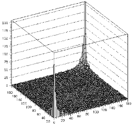
Figure 15: The production angle (in degrees) for the hadron containing a $b$ quark plotted versus the production angle for a hadron containing $\bar{b}$ quark. (For the Tevatron.)

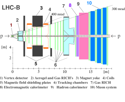
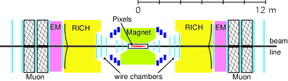
Figure 16: Schematic view of the LHCb (a) and BTeV (b) detectors

The conclusions that we can draw from these data is that dedicated $B$ experiments at hadron colliders are specially suited to pursue this physics with the highest prospects of success. Two such experiments have been proposed, LHCb at the LHC and BTeV at Fermilab. These detectors are shown in Fig. 16 a) and b) respectively. LHCb has been approved, while BTeV is an approved R&D project; they have been invited to submit a proposal in the summer of 2000. Both these experiments exploit the high cross section for beauty production at hadronic machines and the advantages of the forward geometry to achieve optimal performance. LHCb exploits the $\approx$ 5 times higher cross section at LHC compared to the Tevatron, due to the higher CM energy.

Both experiments feature excellent hadron identification. However, they differ in their implementation of some key detector components. BTeV is planning to build a state of the art vertex detector based on high granularity pixel sensors that are used in the first level trigger. LHCb is considering microstrip silicon trackers whose information is used only at a higher trigger level. Furthermore BTeV has proposed an excellent crystal calorimeter based on PbWO₄, whereas LHCb will use a much more modest Shaslik calorimeter. The difference in the quality of the electromagnetic calorimeter is reflected by the difference in the projected sensitivities for the decay $B^{o}\rightarrow\rho^{\pm}\pi^{\mp}$, where LHCb claims an efficiency of $1.7\times 10^{-4}$ [127], whereas BTeV projects and efficiency of $(1.0\pm 0.2)$% [128]. Taking into account the difference in production cross section, the ratio between the projected yields per year in the two experiments favor BTeV with a ratio 12:1 with respect to LHCb [128].

Table 12: Sensitivies for BTeV running for one year and ${\cal L}=2\times 10^{32}\ cm^{-2}s^{-1}$ and LHCb. The LHCb sensitivity numbers have been taken from their Technical Design Report [127] and the BTeV numbers from their Preliminary Technical Design Report [128].

Measurement	BTeV	LHCb
$x_{s}$	$>80$	$>74$
CP asy ($B^{o}\rightarrow\pi^{+}\pi^{-}$)	$\pm 0.032$	$\pm 0.034$
$\gamma(D_{s}K)\dagger$	$\pm 11^{\circ}$	$\pm 6.1^{\circ}-\pm 13^{\circ}$
$\gamma(D^{o}K)$	$\pm 13^{\circ}$
$\gamma(D^{o}K^{\star})$		$\pm 10^{\circ}$

$\dagger$ Both simulations assume $x_{s}=20$. The range of LHCb sensitivity corresponds to different assumptions on the strong and weak phases between the amplitudes $<f|\overline{B}>$ and $<f|B>$.

Table 12 summarizes the expected physics reach of BTeV and LHCb for some key measurements in a year of running. Their competitive effort will insure a detailed and precise exploration of $b$ and $c$ decays and one of the most thorough tests of the Standard Model in a sector where there is a stronger motivation for new physics.

7 Conclusions

The examples discussed in this paper show that much progress has been made in the field of flavour physics. However, we have not accomplished our main goals. The new experiments being planned to do high precision studies of beauty and charm, BTeV and LHCb, have the opportunity of providing crucial information to address the puzzle of flavour and CP violation. In parallel, the study of rare $K$ decays can uncover complementary information on CP violation and ATLAS and CMS will explore the mechanism of electroweak symmetry breaking and maybe find some evidence for supersymmetry. In parallel, the experimental progress will be undoubtely matched by a refinement of theoretical tools. Thus the mystery of flavour may be finally uncovered.

8 Acknowledgements

I would like to thank the organizers of this conference for a very enjoyable and interesting conference. While preparing this manuscript, I have benefited from several interesting discussions with Sheldon Stone, Tomasz Skwarnicki, Zoltan Ligeti, Ikaros Bigi, Matthias Neubert and Amarjit Soni.

References

- [1] Jung C K 1999 These proceedings
- [2] Fayet P and Ferrara S 1977 Phys. Rep. 32c 249; Haber H E amd Kane K L 1987 Phys. Rep. 117C 1
- [3] Kaplan D B, Lepeintre F and Schmaltz M 1997 Phys. Rev. D 56 7193
- [4] Ringwald, Scherempp and Wetterich C 1991 Nucl. Phys. B 365 3
- [5] Sakharov A D 1991 Sov.Phys.Usp. 34417
- [6] Farrar G 1995 Nucl. Phys. Proc. Suppl. 43 312
- [7] Abe F et al. 1995 Phys. Rev. Lett. 74 2626; Abachi S et al. 1995 Phys. Rev. Lett. 74 2632
- [8] Dawson S 1996 in Lectures given at NATO Advanced Study Institute on Techniques and Concepts of High-energy Physics, St. Croix, U.S. Virgin Islands
- [9] Barbaro Galtieri A 1999 FERMILAB-CONF-99/246
- [10] Bigi I I et al. in B Decays, 2nd ed. (Singapore: World Scientific)
- [11] Bigi I I et al. 1994 Phys. Rev. D 50 2234
- [12] Beneke M and Braun V M 1994 Nucl. Phys. B 426 301
- [13] Hashimoto S 1999 Invited talk at Lattice99, Pisa, Italy
- [14] Melnikov K and Yelkhovsky 1999 Phys. Rev. D 59 114009
- [15] Hoang H 1999 Phys. Rev. D 59 014039
- [16] Beneke M, Signer A and Smirnov V A 1999 CERN-TH/98399; hep-ph 9906476
- [17] Kühn J H, Penin A A and Pivovarov A A 1998 TTP98-01; hep-ph/9801356
- [18] Jamin M and Pich A 1997 Nucl. Phys. B 507 334
- [19] Pineda A and Yndurain F J 1998 CERN-TH/98-402; hep-ph/9812371
- [20] Davies et al. 1994 Phys. Rev. Lett. 73 2654
- [21] Martinelli G and Sachrajda C T ROME1-1234/98; hep-lat/9812001
- [22] Wolfenstein L 1983 Phys. Rev. Lett. 51 1945
- [23] Aleksan R, Kayser B and London D 1994 Phys. Rev. Lett. 73 18
- [24] Silva J P and Wolfenstein L 1997 Phys. Rev. D 55 5331
- [25] Buchalla G These proceedings
- [26] Isgur N and Wise M B 1994 in B decays, 2nd Edition (Singapore:World Scientific)
- [27] Neubert M 1991 Phys. Lett. B 341 367
- [28] Czarnecki A 1996 Phys. Rev. Lett. 76 4124
- [29] Falk A F and Neubert M 1003 Phys. Rev. D 47 2965 and 2982
- [30] Mannel T 1995 Phys. Rev. D 50 428
- [31] Shifman M, Uraltsev N G and Vainshtein A 1995 Phys. Rev. D 51 2217
- [32] Neubert M 1994 Phys. Lett. B 338 84
- [33] Boyd C G and Rothstein I Z 1997 Phys. Lett. B 395 96
- [34] Harrison P F and Quinn H R, editors The BaBar Physics Book
- [35] Simone J et al. 1999 FERMILAB-Conf-99/291-T; hep-lat/9910026
- [36] Hashimoto S et al. 1999 FERMILAB-Pub-99/001-T; hep-lat/9906376
- [37] Buskulic D et al. 1997 Phys. Lett. B 395 373
- [38] DELPHI coll 1999 DELPHI 99-107
- [39] Akerstaff et al. 1997 Phys. Lett. B 395 128
- [40] Barish B et al. 1995 Phys. Rev. D 51 1014
- [41] Stone S 1994 Proceedings of DPF Meeting, Albuquerque, NM
- [42] Barish B et al. 1996 Phys. Rev. Lett. 76 1570
- [43] http://home.cern.ch/LEPHFS
- [44] Buskulic D et al. 1995 Phys. Lett. B 359 236
- [45] Abreu P et al. 1996 Z. Phys. C 71 539
- [46] The L3 Collaboration (1999) CERN-EP/99-121
- [47] Abbiendi G et al. 1999 CERN-EP/99-078
- [48] Bigi I I, Shifman M and Uraltsev N G 1997 Annu. Rev. Nucl. Part. Sci. 47 591; Uraltsev N G 1998 in Proc. of the International School of Physics “Enrico Fermi”, Varenna, Italy
- [49] Falk A, Luke M and Savage M J 1996 Phys. Rev. D 53 6316
- [50] Hoang A H et al. 1999 Phys. Rev. Lett. 82 277
- [51] Bigi I I 1999 Contributed Paper to Workshop on the Derivation of and , CERN; hep-ph/9903258
- [52] Voloshin M B 1995 Phys. Rev. D 51 4934
- [53] Isgur N 1998 Jlab-Thy-98-03; hep-ph/9809279
- [54] Bartelt J et al. 1998 CLEO CONF 98-21
- [55] Del Rebbio L et al. 1998 Phys. Lett. B 436 392
- [56] Ball P and Braun V M 1998 Phys. Rev. D 58 094016
- [57] Isgur N and Scora D 1995 Phys. Rev. D 52 2783
- [58] Fulton R et al. 1990 Phys. Rev. Lett. 64 16; Albrecht H et al. 1990 Phys. Lett. B 234 409; ALbrecht H et al. 1991 Phys. Lett. B 255 297; Bartelt J et al. 1993 Phys. Rev. Lett. 71 4111
- [59] Behrens B H et al. 1999 CLNS 99/1611
- [60] Alexander J P et al. 1996 Phys. Rev. Lett. 77 5000
- [61] Beyer M and Melikhov D 1998 Phys. Lett. B 436 344
- [62] Kagan A L and Neubert M 1998 Phys. Rev. D 58 094012; Aoki M, Cho G and Oshimo N 1999 Phys. Rev. D 60 035004, 1998 Phys. Lett. B 436 344
- [63] Ligeti Z and Wise M 1996 Phys. Rev. D 53 4937
- [64] Fulton R et al. 1990 Phys. Rev. Lett. 64 16; Bartelt J et al. 1993 Phys. Rev. Lett. 71 4111
- [65] Artuso M 1996 Nucl. Instr. Meth. 384 39
- [66] Bigi I, Dikeman R D and Uraltsev N 1998 Eur. Phys. J. C 4 453
- [67] LEPVUB/99-01 1999, accessible through www.cern.ch/LEPHFS/
- [68] Ligeti Z 1999 Invited Talk at DPF99, Los Angeles, CA; hep-ph/9904460
- [69] Neubert M 1997 in Heavy Flavours II (Singapore: World Scientific)
- [70] Hamzaoui C et al. 1987 in Proceedings of the Workshop on High Sensitivity Beauty Physics at Fermilab
- [71] Buras A Private Communication
- [72] Alavi-Harati A et al. 199 Phys. Rev. Lett. 83 2128
- [73] The NA48 Collaboration 1999 CERN-ep-99-114
- [74] Buras A J 1999 Invited Talk at KAon 99, Chicago, IL hep-ph/9908395
- [75] Blum T et al. 1999 BNL-66731; hep-lat/9908025
- [76] Ciuchini M et al. Invited Talk at Kaon 99, Chicago, IL; hep-ph/9910237
- [77] http://www.cern.ch/LEPBOSC/
- [78] Sachrajda C T and Flynn J M 1997 in Heavy Flavours II (Singapore: World Scientific). Ryan S 1999 Nucl. Phys. Proc. Suppl. 73 390; hep-lat/9910010.
- [79] Stone S 1999 Invited talk at the 8th International Symposium on Heavy Flavour Physics; hep-ph/9910417
- [80] Stocchi A and Roudeau P 1999 LAL-99-03, hep-ex/9903063
- [81] Barbieri R, Hall L J and Romanino A, 1999 Nucl. Phys. B 551 93
- [82] Fritzsch H and Xing Z 1997 Phys. Lett. B 413 396
- [83] Ahmed S et al. 1999 it CLEO CONF 99-10; hep-ex/9908022
- [84] The ALEPH Collaboration 1998 Phys. Lett. B 429 169
- [85] Chetyrkin K et al. 1997 Phys. Lett. B 400 206;1998 Phys. Lett. B 425 414; Kagan A and Neubert M 1999 Eur. Phys. J. C75
- [86] Alam M S et al. 1995 Phys. Rev. Lett. 74 2885
- [87] Masiero A and Silvestrini L 1996 Nucl. Instr. Meth. 384 34
- [88] Ali A, Hiller G, Handoko L T and Morozumi T 1997 Phys. Rev. D 55 4105
- [89] Abbott B et al. 1998 Phys. Lett. B 423 419
- [90] Glenn S et al. 1998 Phys. Rev. Lett. 80 2289
- [91] Abe F et al. 1999 Phys. Rev. Lett. 76 4675
- [92] Godang R et al. 1998 CLEO CONF 98-22
- [93] Asner D M et al. 1996 Phys. Rev. D 53 1039
- [94] Bishai M et al. 1999 CLEO CONF 99-13; hep-ex/9908018
- [95] Chau L L et al. 1991 Phys. Rev. D 43 2176
- [96] Deandrea A et al. 1993 Phys. Lett. B 318 549; 1994 Phys. Lett. B 320 170
- [97] Du D and Guo L 1997 Z. Phys. C 75 9 75, 9 (1997).
- [98] Deshpande N G, Dutta B and Oh S 1998 Phys. Rev. D 57 5723
- [99] Ciuchini M et al. 1998 Nucl. Phys. B 512 3
- [100] Ali A, Kramer G and Lu C D 1999 Phys. Rev. D 59 014005
- [101] Chen Y T et al. 1999 Phys. Rev. D 60 094014
- [102] Kramer G, Palmer W F, and Simma H, 1995 Z. Phys. C 66 429
- [103] Kramer G, Palmer W F and Simma H, 1994 Nucl. Phys. B 428 429
- [104] Ebert D, Faustov R N and Galkin V O 1997 Phys. Rev. D 56 312
- [105] Deshpande N G and Trampetic J 1990 Phys. Rev. D 41 895
- [106] Du D and Xing Z 1993 Phys. Lett. B 312 199
- [107] Fleischer R 1993 Z. Phys. C 58 483; 1994 Phys. Lett. B 332 419
- [108] Davies A J et al. 1994 Phys. Rev. D 49 5882
- [109] Snyder A E and Quinn H R 1993 Phys. Rev. D 48 2139
- [110] Richichi S J et al. 1999 CLEO CONF 99-12; hep-ex/9908019
- [111] Beherens B H et al. 1998 Phys. Rev. Lett. 80 3710
- [112] Gao Y, Sun W and Würthwein F 1999 talks presented at DPF99 and APS99; hep-ex/9904008v2
- [113] Neubert M 1999 invited talk presented at the 8th International Symposium on Heavy Flavour Physics; hep-ph/9911253 and references therein.
- [114] Atwood D and Soni A 1998 BNL-HET 98-47; hep-ph/9812444, revised in 1999 to include new experimental information
- [115] Hou W S, Smith J G and Würthwein F 1999 COLO-HEP-438; hep-ex/9910014
- [116] Gronau M and Rosner J L TECHNION-PH-99-33; hep-ph/9909478
- [117] A sample of the various theories proposed can be found in: Halperin I and Zhitnitsky T 1997 Phys. Rev. D56 7247 ; Yuan F Chao K T 1997 Phys. Rev. D 56 2495; Atwood D and Soni A 1997 Phys. Lett. B 405 150
- [118] Hewett J L, Takeuchi T and Thomas S 1996 in Electroweak Symmetry Breaking and Beyond the Standard Model
- [119] Aitala E M et al.(E791)1999 Phys. Lett. B 462 401
- [120] Pedrini D 1999 Invited talk at Kaon’99, Chicago, IL
- [121] Caso C et al.1998 The European Physical Journal C 3 1
- [122] Buccella F 1995 Phys. Rev. D 51 3478
- [123] Artuso M et al. 1999 CLEO CONF 99-17; hep-ex/9908040
- [124] Aitala E M et al. 1996 Phys. Rev. Lett. 77 2384
- [125] T. Affolder et al. 1999 FERMILAB-PUB-99/225-E; hep-ex/9909003
- [126] Artuso M 1994 in B decays, 2nd Edition (Singapore: World Scientific)
- [127] Harnew N 1999 invited talk presented at the 8th International Symposium on Heavy Flavour Physics; http://lhcb.cern.ch/
- [128] http://www-btev.fnal.gov/btev.html