What Will the First Year of SNO Show?

Abstract

The ratio of the measured to the predicted standard model CC event rates in SNO will be 0.47 if no oscillations occur. The best-fit active oscillation predictions for the CC ratio are: $0.35-39$ (MSW) and $0.38-42$ (vacuum) (all for a $5$ MeV energy threshold), typically about $20$% less than the no-oscillation expectation. We calculate the predicted ratios for six active and sterile neutrino oscillation solutions allowed at 99% CL and determine the dependence of the ratios on energy threshold. If the high-energy anomaly observed by SuperKamiokande is due to an enhanced $hep$ flux, MSW active solutions predict that out of a total of $5000$ CC events above $5$ MeV in SNO between $49$ and $54$ events will be observed above $13$ MeV whereas only $19$ events are expected for no-oscillations and a nominal standard $hep$ flux.

1 Introduction

The Sudbury Neutrino Observatory (SNO) has been designed to provide definitive answers regarding neutrino properties that are manifested in solar neutrino experiments [1].

What will the first year of SNO show? We answer this question assuming that SNO will detect [1] $\sim 3000$ to $5000$ neutrino absorption (CC) events in the first year and that one of the currently-favored neutrino oscillation solutions is correct.

We focus on CC rate measurements that can be completed in the first year of operation of SNO. Accurate measurements of the energy spectrum, of time-dependences, and of the neutral current will require more time. We begin by determining in Sec. 2 the currently allowed MSW and vacuum oscillation solutions and by showing that the no-oscillation hypothesis is rejected at a high CL even if solar neutrino fluxes are treated as free parameters. In Sec. 3 we show that a “smoking gun” indication of neutrino oscillations may be obtained by measuring the total CC rate (neutrino absorption) in conjunction with the SuperKamiokande measurement [2] of the $\nu-e$ scattering rate. This idea has been discussed previously (see, e. g., refs. [1, 2, 3]). What is new here is the calculation of the expected range of the CC rate for each of the currently favored oscillation solutions. Figure 2 summarizes our most important results. In Sec. 4 we calculate the number of high energy ($>13$ MeV) CC events that are expected if the high-energy anomaly observed by SuperKamiokande [2] is due to an enhanced $hep$ flux. The discussions in refs. [1, 2, 3, 4, 5, 6] describe other things that can be learned by comparing in detail the results of the SuperKamiokande and SNO measurements.

Table 1: Best-fit global oscillation parameters and confidence limits. The active neutrino solutions are from Fig. 1. The differences of the squared masses are given in ${\rm eV^{2}}$.

Scenario	$\Delta m^{2}$	$\sin^{2}(2\theta)$	C.L.
LMA	$2.7\times 10^{-5}$	$7.9\times 10^{-1}$	$68$%
SMA	$5.0\times 10^{-6}$	$7.2\times 10^{-3}$	$64$%
LOW	$1.0\times 10^{-7}$	$9.1\times 10^{-1}$	$83$%
${\rm VAC_{S}}$	$6.5\times 10^{-11}$	$7.2\times 10^{-1}$	$90$%
${\rm VAC_{L}}$	$4.4\times 10^{-10}$	$9.0\times 10^{-1}$	$95$%
${\rm Sterile}$	$4.0\times 10^{-6}$	$6.6\times 10^{-3}$	$73$%

2 Allowed solutions

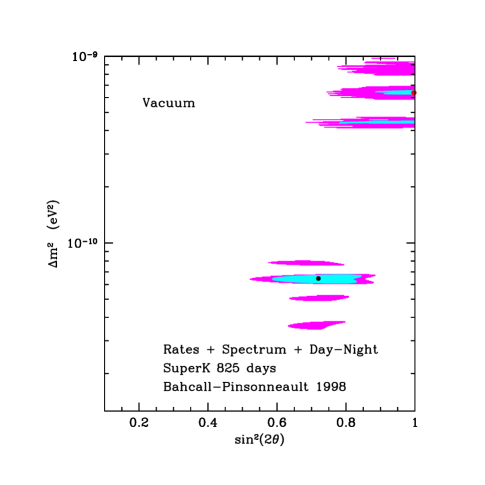
Figure 1 shows the allowed global solutions for MSW [7] and vacuum [8] two-neutrino oscillations. Table 1 gives the best-fit parameters and confidence limits (C.L.) for the different neutrino scenarios, including sterile neutrinos (not shown in Fig. 1 since the allowed region is similar to the SMA region,[9]). The experimental data include the total rates for the Homestake (chlorine) experiment [10], the SAGE [11] and GALLEX [12] (gallium) experiments, and the SuperKamiokande (water Cherenkov) [2] experiment. We also include the SuperKamiokande [2] electron recoil energy spectrum and the difference between the average day and night event rates. We follow the procedures described in our earlier work on global solar neutrino solutions [9]. The vacuum solutions that correspond to a mass smaller than $10^{-10}{\rm eV^{2}}$,${\rm VAC_{S}}$ , fit somewhat better to the total rates (ignoring the spectrum measurement) than the larger-mass solutions, ${\rm VAC_{L}}$. The spectrum is better fit by the larger-mass solutions. The ${\rm VAC_{L}}$ solutions, but not the ${\rm VAC_{S}}$ solutions, predict large seasonal variations for the ⁷Be and pp neutrinos. The predicted seasonal and day-night effects for the ⁸B neutrinos are small for all of the oscillation scenarios.

Figure 1: Global oscillation solutions. The input data include the total rates in the Homestake, Sage, Gallex, and SuperKamiokande experiments, as well as the electron recoil energy spectrum and the Day-Night effect measured by SuperKamiokande in 825 days of data taking. Figure 1a shows the global solutions for the allowed MSW oscillation regions, known, respectively, as the SMA, LMA, and LOW solutions [9]. Figure 1b shows the global solution for the allowed vacuum oscillation regions. The CL contours correspond, for both panels, to $\chi^{2}=\chi^{2}_{\rm min}+4.61(9.21)$, representing 90% ( 99% CL) relative to each of the best-fit solutions (marked by dark circles) given in Table 1. The best vacuum fit to the SuperKamiokande electron recoil energy spectrum is marked in Fig. 1b at $\Delta m^{2}=6.3\times 10^{-10}$ eV² and $\sin^{2}2\theta=1$.

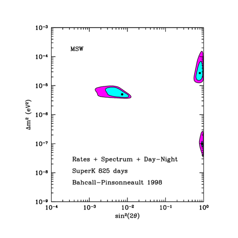
Is there any way, even very artificial, of avoiding the conclusion that some new physics is required to explain the solar neutrino experimental results? We adopt the maximally skeptical attitude and ignore everything we have learned about the sun and about solar models over the past four decades. We allow [9, 13] the $pp$, ${\rm{}^{7}Be}$, ${\rm{}^{8}B}$, and CNO fluxes to take on any non-negative values, requiring only that the shape of the continuum spectra be unchanged (as demanded by standard electroweak theory). The sole constraint on the fluxes is the requirement that the luminosity of the sun be supplied by nuclear fusion reactions among light elements (see section 4 of Ref. [14]); we use the standard value for the essentially model-independent ratio of $pep$ to $pp$ neutrino fluxes.

The search for the best fit fluxes yields: ${\rm{}^{7}Be/(^{7}Be)}_{\rm SM}=0.0$, ${\rm{}^{8}B/(^{8}B)}_{\rm SM}=0.47$, $pp/(pp)_{\rm SM}=1.10$, and CNO/${\rm CNO_{\rm SM}=0.0}$, where SM stands for the combined standard solar [15] and electroweak model. These values were found by an extensive computer search with four free parameters and the luminosity constraint. The minimum value of $\chi^{2}$ is, for 3 d.o.f.,

$$\chi^{2}_{\rm min}\hbox{( {\rm five rates + D-N effect}; ~{}arbitrary $pp$, ${\rm{}^{7}Be}$, ${\rm{}^{8}B}$; CNO)}=13.8\ .$$ (1)

There are no acceptable solutions at the $99.7$% C. L. ($3\sigma$). We carried out searches using a variety of other prescriptions: ab initio setting the CNO fluxes equal to zero, combining the two gallium experiments, and including or excluding the Homestake [10] or Kamiokande [16] experiments. The poor fit is robust. In all cases, there are no acceptable solutions at a CL of about $3\sigma$ or higher. If new physics is required to describe solar neutrino propagation, then this result can be strengthened in the future by adding new results from SNO.

3 SNO versus SuperKamiokande

Let

$$R~{}\equiv~{}\frac{{\rm Observed~{}Rate}}{{\rm Standard~{}Model~{}Rate}}$$ (2)

be the dimensionless ratio of the observed rate (in any experiment) divided by the rate expected from the combined standard solar and electroweak model(SM). The experimental result for SuperKamiokande after 825 days of data taking with a 6.5 MeV energy threshold is [2]

$$R_{\rm SK}=0.475\pm 0.015.$$ (3)

The neutrino-electron scattering experiments, Kamiokande and SuperKamiokande, contain contributions from both charged current and neutral current interactions. Hence, for SuperKamiokande the ratio of observed to standard rates can be written

$$\!\!\!\!\!\!\!\!\!\!\!R_{\rm SK}\!\!=\!\!\frac{f_{B}\int dE_{e}\epsilon(E_{e})\int dE\phi_{\rm SM}(E)\left[\sigma_{\nu_{e}-e}(E,E_{e})P(E)\!+\!\sigma_{\nu_{\mu}-e}(E,E_{e})(1\!\!-\!\!P(E))\right]}{\int dE_{e}\epsilon(E_{e})\int dE\phi_{\rm SM}(E)\sigma_{\nu_{e}-e}(E,E_{e})},\!\!\!\!\!$$

(4)

where $\phi_{\rm SM}(E)$ is the standard model ⁸B neutrino flux, $P(E)=P(E,\nu_{e}\rightarrow\nu_{e})$, $\sigma_{\nu_{e}-e}$ and $\sigma_{\nu_{\mu}-e}$ are the scattering cross sections [17], $E_{e}$ is the electron energy, and $\epsilon(E_{e})$ is the integrated resolution and efficiency function, and $f_{B}$ is defined by

$$f_{B}~{}=~{}{{\phi(^{8}B)_{\rm true}}\over{\phi(^{8}B)_{\rm SM}}}.$$ (5)

Neutrino absorption in SNO is a pure charged-current reaction. Therefore,

$$R_{\rm CC,SNO}=\frac{f_{B}\int dE_{e}\epsilon(E_{e})\int dE\phi_{\rm SM}(E)\left[\sigma_{{\rm abs}}(E,E_{e})P(E)\right]}{\int dE_{e}\epsilon(E_{e})\int dE\phi_{\rm SM}(E)\sigma_{{\rm abs}}(E,E_{e})},$$ (6)

where $\sigma_{\rm abs}$ is the absorption cross section. Equation (4) and Eq. (6) are independent of the total flux $\phi_{\rm SM}$. In intermediate calculations, we use the Bahcall-Pinsonneault 1998 value for the standard model ⁸B flux: $5.15\times 10^{6}{\rm cm^{-2}s^{-1}}$ [15]. For the no-oscillation hypothesis, $f_{B}$ is determined by SuperKamiokande measurements, $f_{B,\rm no~{}oscillation}=0.475$.

The standard electroweak model, which embodies the no neutrino oscillation hypothesis, predicts that

$$R_{\rm SK}~{}=~{}R_{\rm CC,SNO},$$ (7)

independent of the SuperKamiokande and SNO energy thresholds. Equation (7) is valid because, in the absence of new electroweak physics like oscillations, the only theoretical reason for $R_{\rm SK}$ or $R_{\rm CC,SNO}$ being different from unity is that the standard solar model neutrino flux is wrong, i. e., $f_{B}\not=1$. Since $R_{\rm SK}$ and $R_{\rm CC,SNO}$ are both proportional to $f_{B}$, Eq. (7) is correct independent of the calculated standard model flux.

Table 2 gives the calculated values of $R_{\rm CC,SNO}$ that are predicted by all of the allowed neutrino oscillation regions shown in Fig. 1 as well as the sterile neutrino solution (see Sec. 2). At each allowed point, the best-fit ratio, $f_{B}$, of observed to SM neutrino flux was determined by minimizing the $\chi^{2}$ fit of the calculated $\nu-e$ electron recoil energy spectrum with respect to the measured SuperKamiokande recoil energy spectrum . The survival probabilities $P(E)$ are determined by the neutrino oscillation parameters. The neutrino absorption cross sections were evaluated using the computer routine (with speed-up modifications) provided by Bahcall and Lisi. We used all three cross section evaluations in the Bahcall-Lisi subroutines [4]; the theoretical uncertainty in $R_{\rm CC,SNO}$ due to the cross section calculations is $\pm 3$% , much smaller than the spread due to the uncertainty in neutrino parameters. We use the preliminary SNO collaboration estimates for the energy resolution, absolute energy scale, and detection efficiencies [4]. Detailed calculations show that uncertainties in these quantities affect the rates by $\sim$ $1$% or $2$%, which is small compared to the total range of the oscillation predictions. Systematic uncertainties ($\sim 3$% for SuperKamiokande) and precise values for the SNO detector characteristics must be determined by measurements with SNO and by detailed Monte Carlo simulations.

Table 2: Predicted charged current rate in the SNO detector. The table shows the predicted ratio, $R_{\rm CC,SNO}$, of the measured $\nu_{e}$ absorption rate to the combined standard model rate for the different neutrino scenarios shown in Fig. 1 and for sterile neutrinos (similar to the global SMA solutions). For no oscillations, $R_{\rm CC,SNO}=R_{\rm SK}=0.47$. The uncertainties indicated result from the variation of the neutrino parameters within the 90% CL (and the 99% CL) globally-allowed regions of Fig. 1. The second, third, and fourth columns were evaluated using a threshold of 5 MeV, 7 MeV, or 8 MeV, respectively, for the total electron energy. The last column gives the range of $f_{B}$ found at $90$% and $99$% CL by fitting to the measured SuperKamiokande recoil energy spectrum at each globally-allowed set of oscillation parameters.

Scenario	$R_{\rm CC,SNO}$	$R_{\rm CC,SNO}$	$R_{\rm CC,SNO}$	$f_{B}$
Threshold	5 MeV	7 MeV	8 MeV
No osc.	$0.475\pm 0.015$	$0.475\pm 0.015$	$0.475\pm 0.015$	$0.475\pm 0.015$
LMA	$0.35_{-0.05(-0.06)}^{+0.01(+0.05)}$	$0.35_{-0.05(-0.06)}^{+0.01(+0.04)}$	$0.35_{-0.05(-0.06)}^{+0.01(+0.04)}$	$1.140^{0.905(0.875)}_{1.325(1.450)}$
SMA	$0.39_{-0.04(-0.07)}^{+0.03(+0.07)}$	$0.42_{-0.03(-0.06)}^{+0.01(+0.05)}$	$0.43_{-0.03(-0.06)}^{+0.01(+0.05)}$	$0.955^{0.62(0.555)}_{1.23(1.290)}$
LOW	$0.38_{-0.03(-0.03)}^{+0.02(+0.02)}$	$0.38_{-0.03(-0.03)}^{+0.02(+0.02)}$	$0.38_{-0.03(-0.03)}^{+0.02(+0.02)}$	$0.995^{0.910(0.885)}_{0.995(1.15)}$
${\rm VAC_{S}}$	$0.38^{+0.04(+0.08)}_{-0.06(-0.07)}$	$0.42^{+0.02(+0.06)}_{-0.05(-0.09)}$	$0.44^{+0.02(+0.05)}_{-0.04(-0.10)}$	$1.005^{0.815(0.600)}_{1.315(1.425)}$
${\rm VAC_{L}}$	$0.42^{+0.02(+0.03)}_{-0.01(-0.04)}$	$0.41^{+0.03(+0.04)}_{-0.02(-0.03)}$	$0.40^{+0.04(+0.07)}_{-0.03(-0.05)}$	$0.785^{0.710(0.690)}_{0.845(0.830)}$
${\rm MSW,Sterile}$	$0.48^{+0.005(+0.01)}_{-0.005(-0.01)}$	$0.50^{+0.02(+0.03)}_{-0.02(-0.03)}$	$0.50^{+0.04(+0.05)}_{-0.01(-0.02)}$	$0.930^{0.630(0.550)}_{1.245(1.415)}$

Figure 2 shows visually the predicted results when $R_{\rm CC,SNO}$ is compared with $R_{\rm SK}$. The error bars in Fig. 2 correspond to the $99$% CL global solution regions of Fig. 1. The statistical uncertainties after one year of CC measurements with SNO are expected to be $\sim 2$%, which is much less than the range in the neutrino predictions.

For oscillations into active neutrinos, Fig. 2 and Table 2 show that $R_{\rm CC,SNO}$ should be significantly different from $R_{\rm SK}$ unless the correct solution lies in a relatively small region of the allowed parameter space for neutrino oscillations. The average value of the best-fit solutions listed in Table 2 is $R_{\rm CC,SNO}=0.38$, which is about $20$% less than no-oscillation value of $0.475$.

Figure 2: Comparison of the CC SNO rate and the no oscillation prediction. The shaded area is the no oscillation prediction based upon the measured SuperKamiokande rate for $\nu-e$ scattering, see Eq. (3) and Eq. (7). The SNO CC ratios, Eq. (6), are shown on the vertical axes for different neutrino scenarios and two different total electron energy thresholds, 5 MeV and 8 MeV. The error bars on the neutrino oscillation results represent the range of values predicted by the 99% CL allowed neutrino oscillation solutions displayed in Fig. 1.

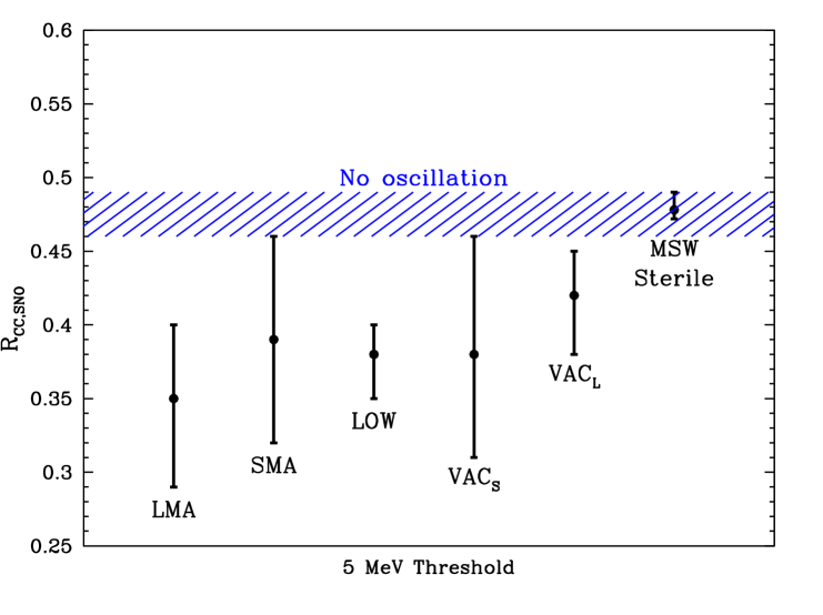
We have evaluated the ratios $R_{\rm CC,SNO}$ for different thresholds in order to exhibit the dependence of the ratios on the threshold energy. A 5 MeV threshold is one of the goals of the SNO collaboration and an 8 MeV threshold would essentially eliminate background from the neutral current reaction, as well as decreasing other troublesome backgrounds [1]. For the LMA and LOW solutions, Fig. 2 and Table 2 show that there is no significant advantage in using a lower threshold, but for the SMA and $VAC_{S}$ solutions there is a substantial improvement in discriminatory power by lowering the threshold from 8 MeV to 5 MeV.

The results for sterile neutrinos are important. One might initially guess that the sterile neutrino solution would give a result very similar to the no-oscillation result. This is the case for a threshold of 5 MeV (see top panel of Fig. 2). However, for an 8 MeV threshold the sterile neutrino solution predicts $R_{\rm CC,SNO}$ that are generally larger than $R_{\rm SK}$ (bottom panel of Fig. 2). The reason is that survival probability for the SMA solution is an increasing function of neutrino energy in the region of interest [9]. If the SMA or sterile neutrino solution is correct, then the 8 MeV threshold measurement will sample on average a higher survival probability than the SuperKamiokande measurement performed with a $6.5$ MeV threshold. In the event that initial measurements performed with an $8$ MeV threshold yield a value of $R_{\rm CC,SNO}$ that is close to or slightly larger than $0.48$, then a measurement of the shape of the recoil electron energy spectrum to as low an energy as possible will be an important test of the predicted small energy dependence of the survival probability of the MSW Sterile solution.

4 The high-energy anomaly in SNO

The recoil energy spectrum measured by SuperKamiokande shows evidence for an enhanced event rate above a total electron energy of $13$ MeV [2] . Several possible explanations for this anomaly have been suggested, including: 1) an enhanced flux of the high energy $hep$ neutrinos [18, 19]; 2) a real upturn in the survival probability that is described by vacuum neutrino oscillations [2]; 3) a statistical fluctuation [2]; and 4) a systematic error in the absolute energy calibration [9]. The first two explanations imply that a high-energy anomaly will also be observed in SNO, while the third and fourth explanations suggest that SNO will not show a high-energy anomaly.

Because of the good intrinsic energy resolution of the deuterium reaction, SNO can discriminate well among these possibilities. To illustrate the sensitivity to the high-energy anomaly, we have computed electron recoil energy spectra in the SNO detector using the best-fit MSW neutrino oscillation scenarios illustrated in Fig. 1 with the $hep$ flux treated as a free parameter.

If the $hep$ flux is equal to the nominal SM value and the electron recoil energy spectrum is not distorted, then $19$ out of a total of $5000$ CC events are expected to be above $13$ MeV. Since the SuperKamiokande measurements have shown a recoil electron spectrum that is not significantly distorted below $13$ MeV, possibilities 3) and 4) also predict about $19$ CC events above $13$ MeV in SNO. The expected number of high energy events is very different if the $hep$ flux is enhanced or if vacuum oscillations cause the high-energy anomaly (possibilities 1 and 2 above).

For different globally-acceptable neutrino oscillation scenarios, Table 3 shows the total number of CC events expected above $13$ MeV and $14$ MeV out of a total of 5000 CC events. For a threshold of $13$ MeV, the difference between the $hep$-enhanced and the non-enhanced energy spectrum is more than $7\sigma$ for the LMA and LOW solutions and about $4.4\sigma$ for the SMA solutions. The two vacuum oscillation regions predict a large range of high-energy events, some of which are not much above the nominal SM solution.

Table 3: High-energy events. The table shows the number of events predicted at large energies out of a total of $5000$ CC events. For all the oscillation scenarios, the $hep$ flux was calculated by evaluating the best-fit value for $\phi({\rm hep})/\phi({\rm hep})_{\rm SM}$ at representative points in the $99$% CL globally allowed regions shown in Fig. 1. For the no-oscillation case, the standard ⁸B spectrum shape was fit to the SuperKamiokande result with the $hep$ flux fixed at the nominal SM value.

Scenario	Events above	Events above	$\phi({\rm hep})/\phi({\rm hep})_{\rm SM}$
	$13$ MeV	$14$ MeV
No osc.	19	4	1
LMA	$51-54$	$22-24$	$27-47$
SMA	$49-53$	$18-23$	$17-19$
LOW	$50-51$	$21-22$	$26-35$
${\rm VAC_{S}}$	$32-54$	$6-23$	$0-40$
${\rm VAC_{L}}$	$22-73$	$3-25$	$0-31$
${\rm MSW\,Sterile}$	$30-43$	8 - 18	$13-25$

5 Discussion: Discovering smoking guns

The standard electroweak model predicts that essentially nothing happens to neutrinos after they are created in the center of the Sun. Solar neutrinos should all be $\nu_{e}$ (produced by beta-decay of proton rich elements) and to high accuracy ($1$ part in $10^{5}$) the ⁸B solar neutrino energy spectrum should have the same shape as the laboratory energy spectrum [20]. Hence, if the standard electroweak model is correct, the ratio, $R_{\rm CC,SNO}$, of the measured neutrino absorption rate in SNO to the rate predicted by the combined standard solar and electroweak model must equal the ratio, $R_{\rm SK}$, of the measured rate in SuperKamiokande to the rate predicted by the combined standard model.

Any departure from this equality, Eq. (7), would be a “smoking gun” indication of new physics. Figure 2 and Table 2 show that SNO has a reasonable chance of discovering this smoking gun in the first year of operation. The mean of the best-fit solutions for oscillating into active neutrinos yields a mean ratio $R_{\rm CC,SNO}$ of $0.38$, which is $20$% less than the no-oscillation expectation of $0.475$. If a smoking-gun is to be discovered, Nature must be reasonably cooperative and not choose an extreme oscillation solution, i. e., an SMA or vacuum solution that produces one of the largest values of $R_{\rm CC,SNO}$ that are allowed by the existing global solutions. If either SMA or vacuum oscillations is the correct solution, then the chances of discovering a smoking gun violation of Eq. (7) would be improved significantly by using a lower threshold like 5 MeV rather than a more easily obtainable threshold like 8 MeV (see Fig. 2 and Table 2). The predictions of the LMA and the LOW solutions are well separated from the measured value of $R_{\rm SK}$ for thresholds between 5 MeV and 8 MeV (cf. Fig. 2).

It will be very difficult to discriminate between different oscillation solutions involving active neutrinos using just measurements of the CC rate. Figure 2 shows that the different oscillation solutions predict largely overlapping values of $R_{\rm CC,SNO}$.

Sterile neutrinos predict values for $R_{\rm CC,SNO}$ that are generally well separated from the solutions for active neutrinos and which show a significant dependence upon energy threshold. For an energy threshold like 8 MeV, the sterile solutions predict values for $R_{\rm CC,SNO}$ that are even larger than the no-oscillation solution (see Fig. 2).

For the six neutrino oscillation scenarios summarized in Table 2, the best-fit total ⁸B flux ranges between $0.79$ and $1.14$ of the standard solar model flux [15]. The globally-allowed solutions span, at $99$% CL, a total range between $0.55$ and $1.32$ of the standard model flux, comparable to the $3\sigma$ model uncertainty.

The high-energy anomaly observed by SuperKamiokande above 13 MeV could be a smoking gun indication of vacuum oscillations [2] or it may be due to a relatively large flux of $hep$ neutrinos [2, 18] or to observational factors [2, 9]. Table 3 summarizes the number of high-energy neutrino events predicted by different neutrino oscillation scenarios. The currently favored MSW solutions predict that between $38$ and $74$ events, out of a total of $5000$ CC events, should be observed above $13$ MeV if there is an enhanced $hep$ flux. Only $19$ out of $5000$ CC events should be above $13$ MeV if the standard electroweak model is correct and the $hep$ is equal to its nominal SM value. Vacuum oscillations allow a wide range, between $24$ and $62$, of higher-energy events.

The results of the first year of operation of SNO will be exciting.

We are grateful to colleagues who made suggestions that improved the initial draft of this paper. JNB acknowledges support from NSF grant No. PHY95-13835 and PIK acknowledges support from NSF grant No. PHY95-13835 and NSF grant No. PHY-9605140. Much of the work for this paper was done while JNB was a visitor in the physics department at the Weizmann Institute of Science and PIK was attending the ‘Neutrino Summer’ program at CERN.

References

- [1] A.B. McDonald, Nucl. Phys. B (Proc. Suppl.) 77 (1999) 43; SNO Collaboration, Physics in Canada 48 (1992) 112; SNO Collaboration, nucl-ex/9910016.
- [2] SuperKamiokande Collaboration, Y. Fukuda et al., Phys. Rev. Lett. 81 (1998) 1158; Erratum 81 (1998) 4279; 82 (1999) 1810; 82 (1999) 2430; Y. Suzuki, Nucl. Phys. B (Proc. Suppl.) 77 (1999) 35; Y. Suzuki, Lepton-Photon ’99, https://www-sldnt.slac.stanford.edu/lp99/db/program.asp .
- [3] Waikwok Kwong, S. P. Rosen, Phys. Rev. D 54 (1996) 2043.
- [4] J.N. Bahcall, E. Lisi, Phys. Rev. D 54 (1996) 5417.
- [5] G.L. Fogli, E. Lisi, D. Montanino, Phys. Lett. B 434 (1998) 333.
- [6] F.L. Villante, G. Fiorentini, E. Lisi, Phys. Rev. D 59 (1999) 013006.
- [7] L. Wolfenstein, Phys. Rev. D 17 (1978) 2369; S.P. Mikheyev, A.Yu. Smirnov, Yad. Fiz. 42 (1985) 1441 [Sov. J. Nucl. Phys. 42 (1985) 913]; Nuovo Cimento C 9 (1986) 17.
- [8] V. N. Gribov and B.M. Pontecorvo, Phys. Lett. B 28 (1969) 493.
- [9] J.N. Bahcall, P.I. Krastev, A.Yu. Smirnov, Phys. Rev. D 58 (1998) 096016; 60 (1999) 93001.
- [10] B.T. Cleveland et al., Astrophys. J. 496 (1998) 505; R. Davis, Prog. Part. Nucl. Phys. 32 (1994) 13.
- [11] SAGE Collaboration, J.N. Abdurashitov et al., astro-ph/9907113 (in press).
- [12] GALLEX Collaboration, W. Hampel et al., Phys. Lett. B 447 (1999) 127.
- [13] K.M. Heeger, R.G.H. Robertson, Phys. Rev. Lett. 77 (1996) 3720; S. Parke, Phys. Rev. Lett. 74 (1995) 839; N. Hata, S. Bludman, and P. Langacker, Phys Rev D 49 (1994) 3622.
- [14] J.N. Bahcall, P.I. Krastev, Phys. Rev. D 53 (1996) 4211.
- [15] J.N. Bahcall, S. Basu, M.H. Pinsonneault, Phys. Lett. B 433 (1998) 1.
- [16] Kamiokande Collaboration, Y. Fukuda et al., Phys. Rev. Lett. 77 (1996) 1683.
- [17] J.N. Bahcall, M. Kamionkowski, A. Sirlin, Phys. Rev. D 51 (1995) 6146.
- [18] J.N. Bahcall, P.I. Krastev, Phys. Lett. B 436 (1998) 243.
- [19] R. Escribano, J.M. Frere, A. Gevaert, D. Monderen, Phys. Lett. B 444 (1998) 397.
- [20] J.N. Bahcall, Phys. Rev. D 45 (1991) 1644.