Two-pearl Strings: Feynman’s Oscillators

Abstract

String models are designed to provide a covariant description of internal space-time structure of relativistic particles. The string is a limiting case of a series of massive beads like a pearl necklace. In the limit of infinite-number of zero-mass beads, it becomes a field-theoretic string. Another interesting limit is to keep only two pearls by eliminating all others, resulting in a harmonic oscillator. The basic strength of the oscillator model is its mathematical simplicity. This encourages us to construct two-pearl strings for a covariant picture of relativistic extended particles. We achieve this goal by transforming the oscillator model of Feynman et al. into a representation of the Poincaré group. We then construct representations of the $O(3)$-like little group for those oscillator states, which dictates their internal space-time symmetry of massive particles. This simple mathematical procedure allows us to explain what we observe in the world in terms of the fundamental space-time symmetries, and the built-in covariance of the model allows us to use the physics in the rest frame in order to explain what happens in the infinite-momentum frame. It is thus possible to calculate the parton distribution within the proton moving light-like speed in terms of the quark wave function in its rest frame.

I Introduction

Physicists are fond of building strings. In classical mechanics, we start with a discrete set of particles joined together with a finite distance between two neighboring particles, like a pearl necklace. We then take the limit of zero distance and infinite number of particles, resulting in a continuous string. This is how we construct classical field theory and then extend it to quantum field theory in the Lagrangian formalism. In this paper, we consider the opposite limit by dropping all the particles except two.

In order to gain an insight into what we intend to in this report, let us note an example in history. Debye’s treatment of specific heat is a classic example. Einstein’s oscillator model of specific heat is a simplified case of the Debye model in the sense that it consists only of two pearls. The Einstein model does not give an accurate description of the specific heat in the zero-temperature limit, but it is accurate enough everywhere else to be covered in textbooks. The basic strength of the oscillator model is its mathematical simplicity. It produces the numbers and curves which can be checked experimentally, without requiring from us too much mathematical labor.

While one of the main purposes of the string models is to study the internal space-time symmetries of relativistic particles, we can achieve this purpose by studying two-pearl strings which should share the same symmetry property as all other string models. In practice, the two-pearl string model consists of two constituents joined together by a spring force. The only problem is to construct the oscillator model which can be Lorentz-transformed. The problem then is to reduced to constructing a covariant harmonic oscillator formalism. This subject has a long history [1, 2, 3, 4].

In Ref. [4], Feynman et al. attempted to construct a covariant model for hadrons consisting of quarks joined together by an oscillator force. They indeed formulated a Lorentz-invariant oscillator equation. They also worked out the degeneracies of the oscillator states which are consistent with observed mesonic and baryonic mass spectra. However, their wave functions are not normalizable in the space-time coordinate system. The authors of this paper never considered the question of covariance.

What is the relevant question on covariance within the framework of the oscillator formalism? In 1969 [5], Feynman proposed his parton model for hadrons moving with almost speed of light. Feynman observed that the hadron consists of collection of infinite number of partons which are like free particles. The partons appear to have properties which are quite different from those of the quarks. If the wave functions are to be covariant, they should be able to translate the quark model for slow hadrons into the parton model of fast hadrons. This is precisely the question we would like to address in the present report.

We achieve this purpose by transforming the oscillator model of Feynman et al. into a representation of the Poincaré group which governs the space-time symmetries of relativistic particles [6, 7]. In this formalism, the internal space-time symmetries are dictated by the little groups. The little group is the maximal subgroup of the Lorentz group whose transformations leave the four-momentum of a given particle invariant. The little groups for massive and massless particles are known to be isomorphic to $O(3)$ or the three-dimensional rotation group and $E(2)$ or the two-dimensional Euclidean group [6, 7]. In this paper, we can rewrite the wave functions of Feynman et al. as a representation of the $O(3)$-like little group for a massive.

Let us go back to physics. When Einstein formulated $E=mc^{2}$ in 1905, he was talking about point particles. These days, particles have their own internal space-time structures. In the case of hadrons, the particle has a space-time extension like the hydrogen atom. In spite of these complications, we do not question the validity of the energy-momentum relation given by $E=\sqrt{m^{2}+p^{2}}$ for all relativistic particles. The problem is that each particle has its own internal space-time variables. In addition to the energy and momentum, the massive particle has a package of variables including mass, spin, and quark degrees of freedom. The massless particle has its helicity, gauge degrees of freedom, and parton degrees of freedom.

The question is whether the two different packages of new variables for massive and massless particles can be combined into a single covariant package as Einstein’s $E=mc^{2}$ does for the energy-momentum relations for massive and massless particles. We shall divide this question into two parts. First, we deal with the question of spin, helicity, and gauge degrees of freedom. We can deal with this question without worrying about the space-time extension of the particle. Second, we face the problem of space-time extensions using hadrons which are bound states of quarks obeying the laws of quantum mechanics. In order to answer this question, we first have to construct a quantum mechanics of bound states which can be Lorentz-boosted.

In Sec. II, the above-mentioned problems are spelled out in detail. In Sec. III, we present a brief history of applications of the little groups of the Poincaré to internal space-time symmetries of relativistic particles. In Sec. IV, we construct representations of the little group using harmonic oscillator wave functions. In Sec. V, it is shown that the Lorentz-boosted oscillator wave functions exhibit the peculiarities Feynman’s parton model in the infinite-momentum limit.

Much of the concept of Lorentz-squeezed wave function is derived from elliptic deformations of a sphere resulting in a mathematical technique group called contractions [8]. In Appendix A, we discuss the contraction of the three-dimensional rotation group to the two-dimensional Euclidean group. In Appendix B, we discuss the little group for a massless particle as the infinite-momentum/zero-mass limit of the little group for a massive particle.

II Statement of the Problem

The Lorentz-invariant differential equation of Feynman, Kislinger, and Ravndal is a linear partial differential equation [4] . It can therefore generate many different sets of solutions depending on boundary conditions. In their paper, Feynman et al. choose Lorentz-invariant solutions. But their solutions are not normalizable and cannot therefore be interpreted within the framework of the existing rules of quantum mechanics. In this report, we point out there are other sets of solutions. We choose here normalizable wave functions. They are not Lorentz-invariant, but they are Lorentz-covariant. These covariant solutions form a representations of the Poincaré group [6, 7].

The Lorentz-invariant wave function takes the same form in every Lorentz frame, but the covariant wave function takes different forms. However, in the covariant formulation, the wave function in one frame can be transformed to the wave function in a different frame by Lorentz transformation. In particular, the wave function in the infinite-momentum frame is quite different from the wave function at the rest frame. Thus, it may be possible to obtain Feynman’s parton picture by Lorentz-boosting the quark wave function constructed from the rest frame.

In spite of the mathematical difficulties, the original paper of Feynman et al. contains the following radical departures from the conventional viewpoint.

• For relativistic bound state, we should use harmonic oscillators instead of Feynman diagrams.

• We should us harmonic oscillators instead of Regge trajectories to study degeneracies in the hadronic spectra.

These views sound radical, but they are quite consistent with the existing forms of quantum mechanics and quantum field theory. In quantum field theory, Feynman diagrams are only for scattering states where the external lines correspond free particles in asymptotic states. The oscillator eigenvalues are proportional to the highest values of the angular momentum. This is often known as the linear Regge trajectory. Between the Regge trajectory and the three-dimensional oscillator, which one is closer to the fundamental laws of quantum mechanics. Therefore, the above-mentioned radical departures mean that we are coming back to common sense in physics.

On the other hand, there is one important point Feynman et al. failed to see in their oscillator paper [4]. Two years before the publication of this oscillator paper, Feynman proposed his parton model [5]. However, in their oscillator paper, they do not mention the possibility of obtaining the parton picture from the quantum mechanics of bound-state quarks in a hadron in its rest frame. It is probably because their wave functions are Lorentz-invariant but not covariant.

However, the covariant formalism forces us to raise this question. This is precisely the purpose of the present report.

III Poincaré Symmetry of Relativistic Particles

The Poincaré group is the group of inhomogeneous Lorentz transformations, namely Lorentz transformations preceded or followed by space-time translations. In order to study this group, we have to understand first the group of Lorentz transformations, the group of translations, and how these two groups are combined to form the Poincaré group. The Poincaré group is a semi-direct product of the Lorentz and translation groups. The two Casimir operators of this group correspond to the (mass)² and (spin)² of a given particle. Indeed, the particle mass and its spin magnitude are Lorentz-invariant quantities.

The question then is how to construct the representations of the Lorentz group which are relevant to physics. For this purpose, Wigner in 1939 studied the subgroups of the Lorentz group whose transformations leave the four-momentum of a given free particle [6]. The maximal subgroup of the Lorentz group which leaves the four-momentum invariant is called the little group. Since the little group leaves the four-momentum invariant, it governs the internal space-time symmetries of relativistic particles. Wigner shows in his paper that the internal space-time symmetries of massive and massless particles are dictated by the $O(3)$-like and $E(2)$-like little groups respectively.

The $O(3)$-like little group is locally isomorphic to the three-dimensional rotation group, which is very familiar to us. For instance, the group $SU(2)$ for the electron spin is an $O(3)$-like little group. The group $E(2)$ is the Euclidean group in a two-dimensional space, consisting of translations and rotations on a flat surface. We are performing these transformations everyday on ourselves when we move from home to school. The mathematics of these Euclidean transformations are also simple. However, the group of these transformations are not well known to us. In Appendix A, we give a matrix representation of the $E(2)$ group.

The group of Lorentz transformations consists of three boosts and three rotations. The rotations therefore constitute a subgroup of the Lorentz group. If a massive particle is at rest, its four-momentum is invariant under rotations. Thus the little group for a massive particle at rest is the three-dimensional rotation group. Then what is affected by the rotation? The answer to this question is very simple. The particle in general has its spin. The spin orientation is going to be affected by the rotation!

If the rest-particle is boosted along the $z$ direction, it will pick up a non-zero momentum component. The generators of the $O(3)$ group will then be boosted. The boost will take the form of conjugation by the boost operator. This boost will not change the Lie algebra of the rotation group, and the boosted little group will still leave the boosted four-momentum invariant. We call this the $O(3)$-like little group. If we use the four-vector coordinate $(x,y,z,t)$, the four-momentum vector for the particle at rest is $(0,0,0,m)$, and the three-dimensional rotation group leaves this four-momentum invariant. This little group is generated by

$$J_{1}=\pmatrix{0&0&0&0\cr 0&0&-i&0\cr 0&i&0&0\cr 0&0&0&0},\qquad J_{2}=\pmatrix{0&0&i&0\cr 0&0&0&0\cr-i&0&0&0\cr 0&0&0&0},$$ (1)

and

$$J_{3}=\pmatrix{0&-i&0&0\cr i&0&0&0\cr 0&0&0&0\cr 0&0&0&0},$$ (2)

which satisfy the commutation relations:

$$[J_{i},J_{j}]=i\epsilon_{ijk}J_{k}.$$ (3)

It is not possible to bring a massless particle to its rest frame. In his 1939 paper [6], Wigner observed that the little group for a massless particle moving along the $z$ axis is generated by the rotation generator around the $z$ axis, namely $J_{3}$ of Eq.(2), and two other generators which take the form

$$N_{1}=\pmatrix{0&0&-i&i\cr 0&0&0&0\cr i&0&0&0\cr i&0&0&0},\quad N_{2}=\pmatrix{0&0&0&0\cr 0&0&-i&i\cr 0&i&0&0\cr 0&i&0&0}.$$ (4)

If we use $K_{i}$ for the boost generator along the i-th axis, these matrices can be written as

$$N_{1}=K_{1}-J_{2},\qquad N_{2}=K_{2}+J_{1},$$ (5)

with

$$K_{1}=\pmatrix{0&0&0&i\cr 0&0&0&0\cr 0&0&0&0\cr i&0&0&0},\qquad K_{2}=\pmatrix{0&0&0&0\cr 0&0&0&i\cr 0&0&0&0\cr 0&i&0&0}.$$ (6)

The generators $J_{3},N_{1}$ and $N_{2}$ satisfy the following set of commutation relations.

$$[N_{1},N_{2}]=0,\quad[J_{3},N_{1}]=iN_{2},\quad[J_{3},N_{2}]=-iN_{1}.$$ (7)

In Appendix A, we discuss the generators of the $E(2)$ group. They are $J_{3}$ which generates rotations around the $z$ axis, and $P_{1}$ and $P_{2}$ which generate translations along the $x$ and $y$ directions respectively. If we replace $N_{1}$ and $N_{2}$ by $P_{1}$ and $P_{2}$, the above set of commutation relations becomes the set given for the $E(2)$ group given in Eq.(A7). This is the reason why we say the little group for massless particles is $E(2)$-like. Very clearly, the matrices $N_{1}$ and $N_{2}$ generate Lorentz transformations.

It is not difficult to associate the rotation generator $J_{3}$ with the helicity degree of freedom of the massless particle. Then what physical variable is associated with the $N_{1}$ and $N_{2}$ generators? Indeed, Wigner was the one who discovered the existence of these generators, but did not give any physical interpretation to these translation-like generators. For this reason, for many years, only those representations with the zero-eigenvalues of the $N$ operators were thought to be physically meaningful representations [9]. It was not until 1971 when Janner and Janssen reported that the transformations generated by these operators are gauge transformations [10, 11]. The role of this translation-like transformation has also been studied for spin-1/2 particles, and it was concluded that the polarization of neutrinos is due to gauge invariance [12, 13].

TABLE I.: Further contents of Einstein’s $E=mc^{2}$. Massive and massless particles have different energy-momentum relations. Einstein’s special relativity gives one relation for both. Wigner’s little group unifies the internal space-time symmetries for massive and massless particles which are locally isomorphic to $O(3)$ and $E(2)$ respectively. It is a great challenge for us to find another unification. In this note, we present a unified picture of the quark and parton models which are applicable to slow and ultra-fast hadrons respectively.

	Massive, Slow	COVARIANCE	Massless, Fast
Energy-		Einstein’s
Momentum	$E=p^{2}/2m$	$E=[p^{2}+m^{2}]^{1/2}$	$E=cp$
Internal	$S_{3}$		$S_{3}$
space-time		Wigner’s
symmetry	$S_{1},S_{2}$	Little Group	Gauge Transformations
Relativistic
Extended	Quark Model	Covariant Model of Hadrons	Partons
Particles

Another important development along this line of research is the application of group contractions to the unifications of the two different little groups for massive and massless particles. We always associate the three-dimensional rotation group with a spherical surface. Let us consider a circular area of radius 1 kilometer centered on the north pole of the earth. Since the radius of the earth is more than 6,450 times longer, the circular region appears flat. Thus, within this region, we use the $E(2)$ symmetry group for this region. The validity of this approximation depends on the ratio of the two radii.

In 1953, Inonu and Wigner formulated this problem as the contraction of $O(3)$ to $E(2)$ [8]. How about then the little groups which are isomorphic to $O(3)$ and $E(2)$? It is reasonable to expect that the $E(2)$-like little group be obtained as a limiting case for of the $O(3)$-like little group for massless particles. In 1981, it was observed by Ferrara and Savoy that this limiting process is the Lorentz boost [14]. In 1983, using the same limiting process as that of Ferrara and Savoy, Han et al showed that transverse rotation generators become the generators of gauge transformations in the limit of infinite momentum and/or zero mass [15]. In 1987, Kim and Wigner showed that the little group for massless particles is the cylindrical group which is isomorphic to the $E(2)$ group [16]. This completes the second raw in Table I, where Wigner’s little group unifies the internal space-time symmetries of massive and massless particles.

We are now interested in constructing the third row in Table I. As we promised in Sec. I, we will be dealing with hadrons which are bound states of quarks with space-time extensions. For this purpose, we need a set of covariant wave functions consistent with the existing laws of quantum mechanics, including of course the uncertainty principle and probability interpretation.

With these wave functions, we propose to solve the following problem in high-energy physics. The quark model works well when hadrons are at rest or move slowly. However, when they move with speed close to that of light, they appear as a collection of infinite-number of partons [5]. As we stated above, we need a set of wave functions which can be Lorentz-boosted. How can we then construct such a set? In constructing wave functions for any purpose in quantum mechanics, the standard procedure is to try first harmonic oscillator wave functions. In studying the Lorentz boost, the standard language is the Lorentz group. Thus the first step to construct covariant wave functions is to work out representations of the Lorentz group using harmonic oscillators [1, 2, 7].

IV Covariant Harmonic Oscillators

If we construct a representation of the Lorentz group using normalizable harmonic oscillator wave functions, the result is the covariant harmonic oscillator formalism [7]. The formalism constitutes a representation of Wigner’s $O(3)$-like little group for a massive particle with internal space-time structure. This oscillator formalism has been shown to be effective in explaining the basic phenomenological features of relativistic extended hadrons observed in high-energy laboratories. In particular, the formalism shows that the quark model and Feynman’s parton picture are two different manifestations of one covariant entity [7, 17]. The essential feature of the covariant harmonic oscillator formalism is that Lorentz boosts are squeeze transformations [18, 19]. In the light-cone coordinate system, the boost transformation expands one coordinate while contracting the other so as to preserve the product of these two coordinate remains constant. We shall show that the parton picture emerges from this squeeze effect.

Let us consider a bound state of two particles. For convenience, we shall call the bound state the hadron, and call its constituents quarks. Then there is a Bohr-like radius measuring the space-like separation between the quarks. There is also a time-like separation between the quarks, and this variable becomes mixed with the longitudinal spatial separation as the hadron moves with a relativistic speed. There are no quantum excitations along the time-like direction. On the other hand, there is the time-energy uncertainty relation which allows quantum transitions. It is possible to accommodate these aspect within the framework of the present form of quantum mechanics. The uncertainty relation between the time and energy variables is the c-number relation [20], which does not allow excitations along the time-like coordinate. We shall see that the covariant harmonic oscillator formalism accommodates this narrow window in the present form of quantum mechanics.

For a hadron consisting of two quarks, we can consider their space-time positions $x_{a}$ and $x_{b}$, and use the variables

$$X=(x_{a}+x_{b})/2,\qquad x=(x_{a}-x_{b})/2\sqrt{2}.$$ (8)

The four-vector $X$ specifies where the hadron is located in space and time, while the variable $x$ measures the space-time separation between the quarks. In the convention of Feynman et al. [4], the internal motion of the quarks bound by a harmonic oscillator potential of unit strength can be described by the Lorentz-invariant equation

$${1\over 2}\left\{x^{2}_{\mu}-{\partial^{2}\over\partial x_{\mu}^{2}}\right\}\psi(x)=\lambda\psi(x).$$ (9)

It is now possible to construct a representation of the Poincaré group from the solutions of the above differential equation [7].

The coordinate $X$ is associated with the overall hadronic four-momentum, and the space-time separation variable $x$ dictates the internal space-time symmetry or the $O(3)$-like little group. Thus, we should construct the representation of the little group from the solutions of the differential equation in Eq.(9). If the hadron is at rest, we can separate the $t$ variable from the equation. For this variable we can assign the ground-state wave function to accommodate the c-number time-energy uncertainty relation [20]. For the three space-like variables, we can solve the oscillator equation in the spherical coordinate system with usual orbital and radial excitations. This will indeed constitute a representation of the $O(3)$-like little group for each value of the mass. The solution should take the form

$$\psi(x,y,z,t)=\psi(x,y,z)\left({1\over\pi}\right)^{1/4}\exp\left(-t^{2}/2\right),$$ (10)

where $\psi(x,y,z)$ is the wave function for the three-dimensional oscillator with appropriate angular momentum quantum numbers. Indeed, the above wave function constitutes a representation of Wigner’s $O(3)$-like little group for a massive particle [7].

Since the three-dimensional oscillator differential equation is separable in both spherical and Cartesian coordinate systems, $\psi(x,y,z)$ consists of Hermite polynomials of $x,y$, and $z$. If the Lorentz boost is made along the $z$ direction, the $x$ and $y$ coordinates are not affected, and can be temporarily dropped from the wave function. The wave function of interest can be written as

$$\psi^{n}(z,t)=\left({1\over\pi}\right)^{1/4}\exp\pmatrix{-t^{2}/2}\psi_{n}(z),$$ (11)

with

$$\psi^{n}(z)=\left({1\over\pi n!2^{n}}\right)^{1/2}H_{n}(z)\exp(-z^{2}/2),$$ (12)

where $\psi^{n}(z)$ is for the $n$-th excited oscillator state. The full wave function $\psi^{n}(z,t)$ is

$$\psi^{n}_{0}(z,t)=\left({1\over\pi n!2^{n}}\right)^{1/2}H_{n}(z)\exp\left\{-{1\over 2}\left(z^{2}+t^{2}\right)\right\}.$$ (13)

The subscript $0$ means that the wave function is for the hadron at rest. The above expression is not Lorentz-invariant, and its localization undergoes a Lorentz squeeze as the hadron moves along the $z$ direction [7]. The above form of the wave function is illustrated in Fig.1.

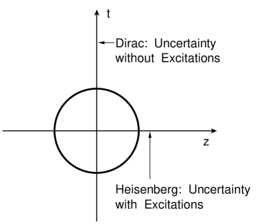
FIG. 1.: Present form of quantum mechanics. There are excitations along the space-like dimensions, but there are no excitations along the time-like direction. However, there still is a time-energy uncertainty relation. We call this Dirac’s c-number time-energy uncertainty relation. It is very important to note that this space-time asymmetry is quite consistent with the concept of covariance

It is convenient to use the light-cone variables to describe Lorentz boosts. The light-cone coordinate variables are

$$u=(z+t)/\sqrt{2},\qquad v=(z-t)/\sqrt{2}.$$ (14)

In terms of these variables, the Lorentz boost along the $z$ direction,

$$\pmatrix{z^{\prime}\cr t^{\prime}}=\pmatrix{\cosh\eta&\sinh\eta\cr\sinh\eta&\cosh\eta}\pmatrix{z\cr t},$$ (15)

takes the simple form

$$u^{\prime}=e^{\eta}u,\qquad v^{\prime}=e^{-\eta}v,$$ (16)

where $\eta$ is the boost parameter and is $\tanh^{-1}(v/c)$. Indeed, the $u$ variable becomes expanded while the $v$ variable becomes contracted. This is the squeeze mechanism illustrated discussed extensively in the literature [18, 19]. This squeeze transformation is also illustrated in Fig. 2.

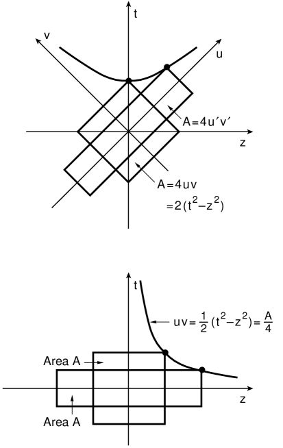
FIG. 2.: Further contents of Lorentz boosts. In the light-cone coordinate system, the Lorentz boost takes the form of the lower part of this figure. In terms of the longitudinal and time-like variables, the transformation is illustrated in the upper portion of this figure.

The wave function of Eq.(13) can be written as

$$\psi^{n}_{o}(z,t)=\psi^{n}_{0}(z,t)=\left({1\over\pi n!2^{n}}\right)^{1/2}H_{n}\left((u+v)/\sqrt{2}\right)\exp\left\{-{1\over 2}(u^{2}+v^{2})\right\}.$$ (17)

If the system is boosted, the wave function becomes

$$\psi^{n}_{\eta}(z,t)=\left({1\over\pi n!2^{n}}\right)^{1/2}H_{n}\left((e^{-\eta}u+e^{\eta}v)/\sqrt{2}\right)\times\exp\left\{-{1\over 2}\left(e^{-2\eta}u^{2}+e^{2\eta}v^{2}\right)\right\}.$$ (18)

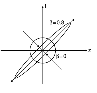
FIG. 3.: Effect of the Lorentz boost on the space-time wave function. The circular space-time distribution at the rest frame becomes Lorentz-squeezed to become an elliptic distribution.

In both Eqs. (17) and (18), the localization property of the wave function in the $uv$ plane is determined by the Gaussian factor, and it is sufficient to study the ground state only for the essential feature of the boundary condition. The wave functions in Eq.(17) and Eq.(18) then respectively become

$$\psi_{0}(z,t)=\left({1\over\pi}\right)^{1/2}\exp\left\{-{1\over 2}(u^{2}+v^{2})\right\}.$$ (19)

If the system is boosted, the wave function becomes

$$\psi_{\eta}(z,t)=\left({1\over\pi}\right)^{1/2}\exp\left\{-{1\over 2}\left(e^{-2\eta}u^{2}+e^{2\eta}v^{2}\right)\right\}.$$ (20)

We note here that the transition from Eq.(19) to Eq.(20) is a squeeze transformation. The wave function of Eq.(19) is distributed within a circular region in the $uv$ plane, and thus in the $zt$ plane. On the other hand, the wave function of Eq.(20) is distributed in an elliptic region. This ellipse is a “squeezed” circle with the same area as the circle, as is illustrated in Fig. 2.

For many years, we have been interested in combining quantum mechanics with special relativity. One way to achieve this goal is to combine the quantum mechanics of Fig. 1 and the relativity of Fig. 2 to produce a covariant picture of Fig. 3. We are now ready to exploit physical consequence of the Lorentz-squeezed quantum mechanics of Fig. 3.

V Feynman’s Parton Picture

It is safe to believe that hadrons are quantum bound states of quarks having localized probability distribution. As in all bound-state cases, this localization condition is responsible for the existence of discrete mass spectra. The most convincing evidence for this bound-state picture is the hadronic mass spectra which are observed in high-energy laboratories [4, 7]. However, this picture of bound states is applicable only to observers in the Lorentz frame in which the hadron is at rest. How would the hadrons appear to observers in other Lorentz frames? More specifically, can we use the picture of Lorentz-squeezed hadrons discussed in Sec. IV.

Proton’s radius is $10^{-5}$ of that of the hydrogen atom. Therefore, it is not unnatural to assume that the proton has a point charge in atomic physics. However, while carrying out experiments on electron scattering from proton targets, Hofstadter in 1955 observed that the proton charge is spread out [21]. In this experiment, an electron emits a virtual photon, which then interacts with the proton. If the proton consists of quarks distributed within a finite space-time region, the virtual photon will interact with quarks which carry fractional charges. The scattering amplitude will depend on the way in which quarks are distributed within the proton. The portion of the scattering amplitude which describes the interaction between the virtual photon and the proton is called the form factor.

Although there have been many attempts to explain this phenomenon within the framework of quantum field theory, it is quite natural to expect that the wave function in the quark model will describe the charge distribution. In high-energy experiments, we are dealing with the situation in which the momentum transfer in the scattering process is large. Indeed, the Lorentz-squeezed wave functions lead to the correct behavior of the hadronic form factor for large values of the momentum transfer [22].

While the form factor is the quantity which can be extracted from the elastic scattering, it is important to realize that in high-energy processes, many particles are produced in the final state. They are called inelastic processes. While the elastic process is described by the total energy and momentum transfer in the center-of-mass coordinate system, there is, in addition, the energy transfer in inelastic scattering. Therefore, we would expect that the scattering cross section would depend on the energy, momentum transfer, and energy transfer. However, one prominent feature in inelastic scattering is that the cross section remains nearly constant for a fixed value of the momentum-transfer/energy-transfer ratio. This phenomenon is called “scaling” [23].

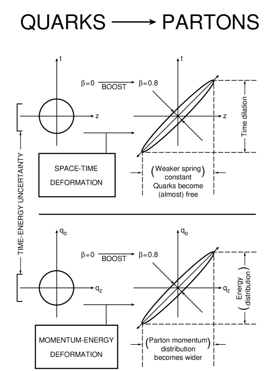
FIG. 4.: Lorentz-squeezed space-time and momentum-energy wave functions. As the hadron’s speed approaches that of light, both wave functions become concentrated along their respective positive light-cone axes. These light-cone concentrations lead to Feynman’s parton picture.

In order to explain the scaling behavior in inelastic scattering, Feynman in 1969 observed that a fast-moving hadron can be regarded as a collection of many “partons” whose properties do not appear to be identical to those of quarks [5]. For example, the number of quarks inside a static proton is three, while the number of partons in a rapidly moving proton appears to be infinite. The question then is how the proton looking like a bound state of quarks to one observer can appear different to an observer in a different Lorentz frame? Feynman made the following systematic observations.

• The picture is valid only for hadrons moving with velocity close to that of light.

• The interaction time between the quarks becomes dilated, and partons behave as free independent particles.

• The momentum distribution of partons becomes widespread as the hadron moves very fast.

• The number of partons seems to be infinite or much larger than that of quarks.

Because the hadron is believed to be a bound state of two or three quarks, each of the above phenomena appears as a paradox, particularly b) and c) together. We would like to resolve this paradox using the covariant harmonic oscillator formalism.

For this purpose, we need a momentum-energy wave function. If the quarks have the four-momenta $p_{a}$ and $p_{b}$, we can construct two independent four-momentum variables [4]

$$P=p_{a}+p_{b},\qquad q=\sqrt{2}(p_{a}-p_{b}).$$ (21)

The four-momentum $P$ is the total four-momentum and is thus the hadronic four-momentum. $q$ measures the four-momentum separation between the quarks.

We expect to get the momentum-energy wave function by taking the Fourier transformation of Eq.(20):

$$\phi_{\eta}(q_{z},q_{0})=\left({1\over 2\pi}\right)\int\psi_{\eta}(z,t)\exp{\left\{-i(q_{z}z-q_{0}t)\right\}}dxdt.$$ (22)

Let us now define the momentum-energy variables in the light-cone coordinate system as

$$q_{u}=(q_{0}-q_{z})/\sqrt{2},\qquad q_{v}=(q_{0}+q_{z})/\sqrt{2}.$$ (23)

In terms of these variables, the Fourier transformation of Eq.(22) can be written as

$$\phi_{\eta}(q_{z},q_{0})=\left({1\over 2\pi}\right)\int\psi_{\eta}(z,t)\exp{\left\{-i(q_{u}u+q_{v}v)\right\}}dudv.$$ (24)

The resulting momentum-energy wave function is

$$\phi_{\eta}(q_{z},q_{0})=\left({1\over\pi}\right)^{1/2}\exp\left\{-{1\over 2}\left(e^{-2\eta}q_{u}^{2}+e^{2\eta}q_{v}^{2}\right)\right\}.$$ (25)

Since we are using here the harmonic oscillator, the mathematical form of the above momentum-energy wave function is identical to that of the space-time wave function. The Lorentz squeeze properties of these wave functions are also the same, as are indicated in Fig. 4.

When the hadron is at rest with $\eta=0$, both wave functions behave like those for the static bound state of quarks. As $\eta$ increases, the wave functions become continuously squeezed until they become concentrated along their respective positive light-cone axes. Let us look at the z-axis projection of the space-time wave function. Indeed, the width of the quark distribution increases as the hadronic speed approaches that of the speed of light. The position of each quark appears widespread to the observer in the laboratory frame, and the quarks appear like free particles.

Furthermore, interaction time of the quarks among themselves become dilated. Because the wave function becomes wide-spread, the distance between one end of the harmonic oscillator well and the other end increases as is indicated in Fig. 4. This effect, first noted by Feynman [5], is universally observed in high-energy hadronic experiments. The period is oscillation is increases like $e^{\eta}$. On the other hand, the interaction time with the external signal, since it is moving in the direction opposite to the direction of the hadron, it travels along the negative light-cone axis. If the hadron contracts along the negative light-cone axis, the interaction time decreases by $e^{-\eta}$. The ratio of the interaction time to the oscillator period becomes $e^{-2\eta}$. The energy of each proton coming out of the Fermilab accelerator is $900GeV$. This leads the ratio to $10^{-6}$. This is indeed a small number. The external signal is not able to sense the interaction of the quarks among themselves inside the hadron.

The momentum-energy wave function is just like the space-time wave function. The longitudinal momentum distribution becomes wide-spread as the hadronic speed approaches the velocity of light. This is in contradiction with our expectation from nonrelativistic quantum mechanics that the width of the momentum distribution is inversely proportional to that of the position wave function. Our expectation is that if the quarks are free, they must have their sharply defined momenta, not a wide-spread distribution. This apparent contradiction presents to us the following two fundamental questions:

• . If both the spatial and momentum distributions become widespread as the hadron moves, and if we insist on Heisenberg’s uncertainty relation, is Planck’s constant dependent on the hadronic velocity?

• . Is this apparent contradiction related to another apparent contradiction that the number of partons is infinite while there are only two or three quarks inside the hadron?

The answer to the first question is “No”, and that for the second question is “Yes”. Let us answer the first question which is related to the Lorentz invariance of Planck’s constant. If we take the product of the width of the longitudinal momentum distribution and that of the spatial distribution, we end up with the relation

$$<z^{2}><q_{z}^{2}>=(1/4)[\cosh(2\eta)]^{2}.$$ (26)

The right-hand side increases as the velocity parameter increases. This could lead us to an erroneous conclusion that Planck’s constant becomes dependent on velocity. This is not correct, because the longitudinal momentum variable $q_{z}$ is no longer conjugate to the longitudinal position variable when the hadron moves.

In order to maintain the Lorentz-invariance of the uncertainty product, we have to work with a conjugate pair of variables whose product does not depend on the velocity parameter. Let us go back to Eq.(23) and Eq.(24). It is quite clear that the light-cone variable $u$ and $v$ are conjugate to $q_{u}$ and $q_{v}$ respectively. It is also clear that the distribution along the $q_{u}$ axis shrinks as the $u$-axis distribution expands. The exact calculation leads to

$$<u^{2}><q_{u}^{2}>=1/4,\qquad<v^{2}><q_{v}^{2}>=1/4.$$ (27)

Planck’s constant is indeed Lorentz-invariant.

Let us next resolve the puzzle of why the number of partons appears to be infinite while there are only a finite number of quarks inside the hadron. As the hadronic speed approaches the speed of light, both the x and q distributions become concentrated along the positive light-cone axis. This means that the quarks also move with velocity very close to that of light. Quarks in this case behave like massless particles.

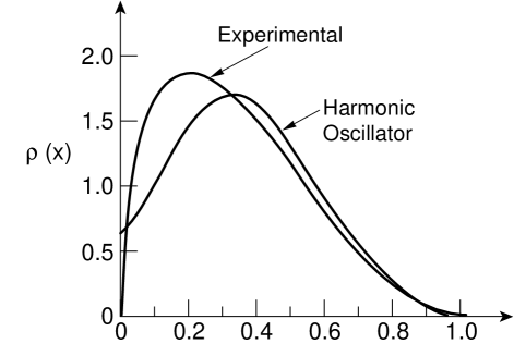
FIG. 5.: Parton distribution. It is possible to calculate the parton distribution from the Lorentz-boosted oscillator wave function. This theoretical curve is compared with the experimental curve.

We then know from statistical mechanics that the number of massless particles is not a conserved quantity. For instance, in black-body radiation, free light-like particles have a widespread momentum distribution. However, this does not contradict the known principles of quantum mechanics, because the massless photons can be divided into infinitely many massless particles with a continuous momentum distribution.

Likewise, in the parton picture, massless free quarks have a wide-spread momentum distribution. They can appear as a distribution of an infinite number of free particles. These free massless particles are the partons. It is possible to measure this distribution in high-energy laboratories, and it is also possible to calculate it using the covariant harmonic oscillator formalism. We are thus forced to compare these two results. Indeed, according to Hussar’s calculation [24], the Lorentz-boosted oscillator wave function produces a reasonably accurate parton distribution, as indicated in Fig. 5

Concluding Remarks

In this report, we have considered a string consisting only of two particles bounded together by an oscillator potential. The essence of the problem was to construct a quantum mechanics of harmonic oscillators which can be Lorentz-transformed. We achieved this purpose by remodeling the oscillator formalism of Feynman, Kislinger and Ravndal. Their Lorentz-invariant equation has a covariant set of solutions which is consistent with the existing principles of quantum mechanics and special relativity.

From these wave wave functions, it is possible to construct a representation of Wigner’s $O(3)$-like little group governing the internal space-time symmetries of relativistic particles with non-zero mass. In order to illustrate the difference between the little group for massive particles from that for massless particles, we have given a comprehensive review of the little groups for massive and massless particles. We have discussed also the contraction procedure in which the $E(2)$-like little group for massless particles is obtained from the $O(3)$-like little group for massive particles. We have given a comprehensive review of the contents of Table I.

Let us go back to the issue of strings. As we noted earlier in this paper, the string is a limiting case of discrete sets of mass points. We can consider two limiting cases, namely the continuous string and two-particle string. There also is a possibility of strings of discrete sets of particles, or “polymers of point-like constituents”[25]. These different strings might take different mathematical forms, but they should all share the space-time symmetry. Thus, the quickest way to study this symmetry is to use the simplest mathematical technique which the two-pearl string provides.

A Contraction of O(3) to E(2)

In this Appendix, we explain what the $E(2)$ group is. We then explain how we can obtain this group from the three-dimensional rotation group by making a flat-surface or cylindrical approximation. This contraction procedure will give a clue to obtaining the $E(2)$-like symmetry for massless particles from the $O(3)$-like symmetry for massive particles by making the infinite-momentum limit.

The $E(2)$ transformations consist of rotation and two translations on a flat plane. Let us start with the rotation matrix applicable to the column vector $(x,y,1)$:

$$R(\theta)=\pmatrix{\cos\theta&-\sin\theta&0\cr\sin\theta&\cos\theta&0\cr 0&0&1}.$$ (A1)

Let us then consider the translation matrix:

$$T(a,b)=\pmatrix{1&0&a\cr 0&1&b\cr 0&0&1}.$$ (A2)

If we take the product $T(a,b)R(\theta)$,

$$E(a,b,\theta)=T(a,b)R(\theta)=\pmatrix{\cos\theta&-\sin\theta&a\cr\sin\theta&\cos\theta&b\cr 0&0&1}.$$ (A3)

This is the Euclidean transformation matrix applicable to the two-dimensional $xy$ plane. The matrices $R(\theta)$ and $T(a,b)$ represent the rotation and translation subgroups respectively. The above expression is not a direct product because $R(\theta)$ does not commute with $T(a,b)$. The translations constitute an Abelian invariant subgroup because two different $T$ matrices commute with each other, and because

$$R(\theta)T(a,b)R^{-1}(\theta)=T(a^{\prime},b^{\prime}).$$ (A4)

The rotation subgroup is not invariant because the conjugation

$$T(a,b)R(\theta)T^{-1}(a,b)$$

does not lead to another rotation.

We can write the above transformation matrix in terms of generators. The rotation is generated by

$$J_{3}=\pmatrix{0&-i&0\cr i&0&0\cr 0&0&0}.$$ (A5)

The translations are generated by

$$P_{1}=\pmatrix{0&0&i\cr 0&0&0\cr 0&0&0},\qquad P_{2}=\pmatrix{0&0&0\cr 0&0&i\cr 0&0&0}.$$ (A6)

These generators satisfy the commutation relations:

$$[P_{1},P_{2}]=0,\qquad[J_{3},P_{1}]=iP_{2},\qquad[J_{3},P_{2}]=-iP_{1}.$$ (A7)

This $E(2)$ group is not only convenient for illustrating the groups containing an Abelian invariant subgroup, but also occupies an important place in constructing representations for the little group for massless particles, since the little group for massless particles is locally isomorphic to the above $E(2)$ group.

The contraction of $O(3)$ to $E(2)$ is well known and is often called the Inonu-Wigner contraction [8]. The question is whether the $E(2)$-like little group can be obtained from the $O(3)$-like little group. In order to answer this question, let us closely look at the original form of the Inonu-Wigner contraction. We start with the generators of $O(3)$. The $J_{3}$ matrix is given in Eq.(2), and

$$J_{2}=\pmatrix{0&0&i\cr 0&0&0\cr-i&0&0},\qquad J_{3}=\pmatrix{0&-i&0\cr i&0&0\cr 0&0&0}.$$ (A8)

The Euclidean group $E(2)$ is generated by $J_{3},P_{1}$ and $P_{2}$, and their Lie algebra has been discussed in Sec. I.

Let us transpose the Lie algebra of the $E(2)$ group. Then $P_{1}$ and $P_{2}$ become $Q_{1}$ and $Q_{2}$ respectively, where

$$Q_{1}=\pmatrix{0&0&0\cr 0&0&0\cr i&0&0},\qquad Q_{2}=\pmatrix{0&0&0\cr 0&0&0\cr 0&i&0}.$$ (A9)

Together with $J_{3}$, these generators satisfy the same set of commutation relations as that for $J_{3},P_{1}$, and $P_{2}$ given in Eq.(A7):

$$[Q_{1},Q_{2}]=0,\qquad[J_{3},Q_{1}]=iQ_{2},\qquad[J_{3},Q_{2}]=-iQ_{1}.$$ (A10)

These matrices generate transformations of a point on a circular cylinder. Rotations around the cylindrical axis are generated by $J_{3}$. The matrices $Q_{1}$ and $Q_{2}$ generate translations along the direction of $z$ axis. The group generated by these three matrices is called the cylindrical group [16, 26].

We can achieve the contractions to the Euclidean and cylindrical groups by taking the large-radius limits of

$$P_{1}={1\over R}B^{-1}J_{2}B,\qquad P_{2}=-{1\over R}B^{-1}J_{1}B,$$ (A11)

and

$$Q_{1}=-{1\over R}BJ_{2}B^{-1},\qquad Q_{2}={1\over R}BJ_{1}B^{-1},$$ (A12)

where

$$B(R)=\pmatrix{1&0&0\cr 0&1&0\cr 0&0&R}.$$ (A13)

The vector spaces to which the above generators are applicable are $(x,y,z/R)$ and $(x,y,Rz)$ for the Euclidean and cylindrical groups respectively. They can be regarded as the north-pole and equatorial-belt approximations of the spherical surface respectively [16].

B Contraction of O(3)-like to E(2)-like Little Groups

Since $P_{1}(P_{2})$ commutes with $Q_{2}(Q_{1})$, we can consider the following combination of generators.

$$F_{1}=P_{1}+Q_{1},\qquad F_{2}=P_{2}+Q_{2}.$$ (B1)

Then these operators also satisfy the commutation relations:

$$[F_{1},F_{2}]=0,\qquad[J_{3},F_{1}]=iF_{2},\qquad[J_{3},F_{2}]=-iF_{1}.$$ (B2)

However, we cannot make this addition using the three-by-three matrices for $P_{i}$ and $Q_{i}$ to construct three-by-three matrices for $F_{1}$ and $F_{2}$, because the vector spaces are different for the $P_{i}$ and $Q_{i}$ representations. We can accommodate this difference by creating two different $z$ coordinates, one with a contracted $z$ and the other with an expanded $z$, namely $(x,y,Rz,z/R)$. Then the generators become

$$P_{1}=\pmatrix{0&0&0&i\cr 0&0&0&0\cr 0&0&0&0\cr 0&0&0&0},\qquad P_{2}=\pmatrix{0&0&0&0\cr 0&0&0&i\cr 0&0&0&0\cr 0&0&0&0}.$$ (B3)

$$Q_{1}=\pmatrix{0&0&0&0\cr 0&0&0&0\cr i&0&0&0\cr 0&0&0&0},\qquad Q_{2}=\pmatrix{0&0&0&0\cr 0&0&0&0\cr 0&i&0&0\cr 0&0&0&0}.$$ (B4)

Then $F_{1}$ and $F_{2}$ will take the form

$$F_{1}=\pmatrix{0&0&0&i\cr 0&0&0&0\cr i&0&0&0\cr 0&0&0&0},\qquad F_{2}=\pmatrix{0&0&0&0\cr 0&0&0&i\cr 0&i&0&0\cr 0&0&0&0}.$$ (B5)

The rotation generator $J_{3}$ takes the form of Eq.(2). These four-by-four matrices satisfy the E(2)-like commutation relations of Eq.(B2).

Now the $B$ matrix of Eq.(A13), can be expanded to

$$B(R)=\pmatrix{1&0&0&0\cr 0&1&0&0\cr 0&0&R&0\cr 0&0&0&1/R}.$$ (B6)

If we make a similarity transformation on the above form using the matrix

$$\pmatrix{1&0&0&0\cr 0&1&0&0\cr 0&0&1/\sqrt{2}&-1/\sqrt{2}\cr 0&0&1/\sqrt{2}&1/\sqrt{2}},$$ (B7)

which performs a 45-degree rotation of the third and fourth coordinates, then this matrix becomes

$$\pmatrix{1&0&0&0\cr 0&1&0&0\cr 0&0&\cosh\eta&\sinh\eta\cr 0&0&\sinh\eta&\cosh\eta},$$ (B8)

with $R=e^{\eta}$. This form is the Lorentz boost matrix along the $z$ direction. If we start with the set of expanded rotation generators $J_{3}$ of Eq.(2), and perform the same operation as the original Inonu-Wigner contraction given in Eq.(A11), the result is

$$N_{1}={1\over R}B^{-1}J_{2}B,\qquad N_{2}=-{1\over R}B^{-1}J_{1}B,$$ (B9)

where $N_{1}$ and $N_{2}$ are given in Eq.(4). The generators $N_{1}$ and $N_{2}$ are the contracted $J_{2}$ and $J_{1}$ respectively in the infinite-momentum/zero-mass limit.

REFERENCES

- [1] P. A. M. Dirac, Proc. Roy. Soc. (London) A183, 284 (1945).
- [2] H. Yukawa, Phys. Rev. 91, 415 (1953).
- [3] M. Markov, Suppl. Nuovo Cimento 3, 760 (1956).
- [4] R. P. Feynman, M. Kislinger, and F. Ravndal, Phys. Rev. D 3, 2706 (1971).
- [5] R. P. Feynman, in High Energy Collisions, Proceedings of the Third International Conference, Stony Brook, New York, edited by C. N. Yang et al. (Gordon and Breach, New York, 1969).
- [6] E. P. Wigner, Ann. Math. 40, 149 (1939).
- [7] Y. S. Kim and M. E. Noz, Theory and Applications of the Poincaré Group (Reidel, Dordrecht, 1986).
- [8] E. Inonu and E. P. Wigner, Proc. Natl. Acad. Sci. (U.S.) 39, 510 (1953).
- [9] S. Weinberg, Phys. Rev. 134, B882 (1964); ibid. 135, B1049 (1964).
- [10] A. Janner and T. Jenssen, Physica 53, 1 (1971); ibid. 60, 292 (1972).
- [11] Y. S. Kim, in Symmetry and Structural Properties of Condensed Matter, Proceedings 4th International School of Theoretical Physics (Zajaczkowo, Poland), edited by T. Lulek, W. Florek, and B. Lulek (World Scientific, 1997).
- [12] D. Han, Y. S. Kim, and D. Son, Phys. Rev. D 26, 3717 (1982).
- [13] Y. S. Kim, in Quantum Systems: New Trends and Methods, Proceedings of the International Workshop (Minsk, Belarus), edited by Y. S. Kim, L. M. Tomil’chik, I. D. Feranchuk, and A. Z. Gazizov (World Scientific, 1997)
- [14] S. Ferrara and C. Savoy, in Supergravity 1981, S. Ferrara and J. G. Taylor eds. (Cambridge Univ. Press, Cambridge, 1982), p. 151. See also P. Kwon and M. Villasante, J. Math. Phys. 29, 560 (1988); ibid. 30, 201 (1989). For an earlier paper on this subject, see H. Bacry and N. P. Chang, Ann. Phys. 47, 407 (1968).
- [15] D. Han, Y. S. Kim, and D. Son, Phys. Lett. B 131, 327 (1983). See also D. Han, Y. S. Kim, M. E. Noz, and D. Son, Am. J. Phys. 52, 1037 (1984).
- [16] Y. S. Kim and E. P. Wigner, J. Math. Phys. 28, 1175 (1987) and 32, 1998 (1991).
- [17] Y. S. Kim, Phys. Rev. Lett. 63, 348-351 (1989).
- [18] Y. S. Kim and M. E. Noz, Phys. Rev. D 8, 3521 (1973).
- [19] Y. S. Kim and M. E. Noz, Phase Space Picture of Quantum Mechanics (World Scientific, Singapore, 1991).
- [20] P. A. M. Dirac, Proc. Roy. Soc. (London) A114, 243 and 710 (1927).
- [21] R. Hofstadter and R. W. McAllister, Phys. Rev. 98, 217 (1955).
- [22] K. Fujimura, T. Kobayashi, and M. Namiki, Prog. Theor. Phys. 43, 73 (1970).
- [23] J. D. Bjorken and E. A. Paschos, Phys. Rev. 185, 1975 (1969).
- [24] P. E. Hussar, Phys. Rev. D 23, 2781 (1981).
- [25] O. Bergman, C. B. Thorn, Nucl. Phys. B 502, 309 (1997).
- [26] Y. S. Kim and E. P. Wigner, J. Math. Phys. 31, 55 (1990).