Kaluza-Klein Physics at
Muon Colliders

Abstract

We discuss the physics of Kaluza-Klein excitations of the Standard Model gauge bosons that can be explored by a high energy muon collider in the era after the LHC and TeV Linear Collider. We demonstrate that the muon collider is a necessary ingredient in the unraveling the properties of such states and, perhaps, proving their existence. The possibility of observing the resonances associated with the excited KK graviton states of the Randall-Sundrum model is also discussed.

Introduction

In theories with extra dimensions, $d\geq 1$, the gauge fields of the Standard Model(SM) will have Kaluza-Klein(KK) excitations if they are allowed to propagate in the bulk of the extra dimensions. If such a scenario is realized then, level by level, the masses of the excited states of the photon, $Z$, $W$ and gluon would form highly degenerate towers. The possibility that the masses of the lowest lying of these states, of order the inverse size of the compactification radius $\sim 1/R$, could be as low as $\sim$ a few TeV or less leads to a very rich and exciting phenomenology at future and, possibly, existing collidersold . For the case of one extra dimension compactified on $S^{1}/Z_{2}$ the spectrum of the excited states is given by $M_{n}=n/R$ and the couplings of the excited modes relative to the corresponding zero mode to states remaining on the wall at the orbifold fixed points, such as the SM fermions, is simply $\sqrt{2}$ for all $n$. These masses and couplings are insensitive to the choice of compactification in the case of one extra dimension assuming the metric tensor factorizes, i.e., the elements of the metric tensor on the wall are independent of the compactified co-ordinates.

If such KK states exist what is the lower bound on their mass? We already know from direct $Z^{\prime}/W^{\prime}$ and dijet bump searches at the Tevatron from Run I that they must lie above $\simeq 0.85$ TeVtev . A null result for a search made with data from Run II will push this limit to $\simeq 1.1$ TeV or so. To do better than this at present we must rely on the indirect effects associated with KK tower exchange in what essentially involves a set of dimension-six contact interactions. Such limits rely upon a number of additional assumptions, in particular, that the effect of KK exchanges is the only new physics beyond the SM. The strongest and least model-dependent of these bounds arises from an analysis of charged current contact interactions at both HERA and the Tevatron by Cornet, Relano and Ricocornet who, in the case of one extra dimension, obtain a bound of $R^{-1}>3.4$ TeV. Similar analyses have been carried out by a number of authorshost ; rw ; the best limit arises from an updated combined fit to the precision electroweak datarw as presented at the 1999 summer conferencesdata and yieldskktest $R^{-1}>3.9$ TeV for the case of one extra dimension. From the previous discussion we can also draw a further conclusion for the case $d=1$: the lower bound $M_{1}>3.9$ TeV is so strong that the second KK excitations, whose masses must now exceed 7.8 TeV due to the above scaling law, will be beyond the reach of the LHC. This leads to the important result that the LHC will at most only detect the first set of KK excitations for $d=1$.

In all analyses that obtain indirect limits on $M_{1}$, one is actually constraining a dimensionless quantity such as

$$V=\sum_{{\bf n}=1}^{\infty}{g_{\bf n}^{2}\over{g_{0}^{2}}}{M_{w}^{2}\over{M_{\bf n}^{2}}}\,,$$ (1)

where, generalizing the case to $d$ additional dimensions, $g_{\bf n}$ is the coupling and $M_{\bf n}$ the mass of the $n^{th}$ KK level labelled by the set of $d$ integers n and $M_{w}$ is the $W$ boson mass which we employ as a typical weak scale factor. For $d=1$ this sum is finite since $M_{n}=n/R$ and $g_{n}/g_{0}=\sqrt{2}$ for $n>1$; one immediately obtains $V={\pi^{2}\over{3}}(M_{w}/M_{1})^{2}$ with $M_{1}$ being the mass of the first KK excitation. From the precision data one obtains a bound on $V$ and then uses the above expression to obtain the corresponding bound on $M_{1}$. For $d>1$, however, independently of how the extra dimensions are compactified, the above sum in $V$ diverges and so it is not so straightforward to obtain a bound on $M_{1}$. We also recall that for $d>1$ the mass spectrum and the relative coupling strength of any particular KK excitation now become dependent upon how the additional dimensions are compactified.

There are several ways one can deal with this divergence: ($i$) The simplest approach is to argue that as the states being summed in $V$ get heavier they approach the mass of the string scale, $M_{s}$, above which we know little and some new theory presumably takes over. Thus we should just truncate the sum at some fixed maximum value $n_{max}\simeq M_{s}R$ so that masses KK masses above $M_{s}$ do not contribute. ($ii$) A second possibility is to note that the wall on which the SM fermions reside is not completely rigid having a finite tension. The authors in Ref.wow argue that this wall tension can act like an exponential suppression of the couplings of the higher KK states in the tower thus rendering the summation finite, i.e., $g_{\bf n}^{2}\rightarrow g_{\bf n}^{2}e^{-(M_{n}/M_{1})^{2}/n_{max}^{2}}$, where $n_{max}$ now parameterizes the strength of the exponential cut-off. (Antoniadiskktest has argued that such an exponential suppression can also arise from considerations of string scattering amplitudes at high energies.) For a fixed value of $n_{max}$, the exponential approach is found to be more effective and lead to a smaller sum than that obtained by simple truncation and thus to a weaker bound on $M_{1}$. ($iii$) A last scenarioschm is to note the possibility that the SM wall fermions may have a finite size in the extra dimensions which smear out and soften the couplings appearing in the sum to yield a finite result. In this case the suppression is also of the Gaussian variety.

We note that in all of the above approaches the value of the sum increases rapidly with $d$ for a fixed value of the cut-off parameter $n_{max}$. For $d=2(>2)$ the sum behaves asymptotically as $\sim log~{}n_{max}(\sim n_{max}^{d-2})$. This leads to the very important result that, for a fixed bound on $V$ from experimental data, the corresponding bound on the mass of the lowest lying KK excitation rapidly strengthens with the number of extra dimension, $d$. Table I shows how the $d=1$ lower bound of 3.9 TeV for the mass of $M_{1}$ changes as we consider different compactifications for $d>1$. We see that in some cases the value of $M_{1}$ is so large it will be beyond the mass range accessible to the LHC as it is for all cases of the $d=3$ example.

Table 1: Lower bound on the mass of the first KK state in TeV resulting from the constraint on $V$ for the case of more than one dimension. ‘T’[‘E’] labels the result obtained from the direct truncation (exponential suppression). Cases labeled by an asterisk will be observable at the LHC. $Z_{2}\times Z_{2}$ and $Z_{3,6}$ correspond to compactifications in the case of $d=2$ while $Z_{2}\times Z_{2}\times Z_{2}$ is for the case of $d=3$.

	$Z_{2}\times Z_{2}$		$Z_{3,6}$		$Z_{2}\times Z_{2}\times Z_{2}$
$n_{max}$	T	E	T	E	T	E
2	5.69∗	4.23∗	6.63∗	4.77∗	8.65	8.01
3	6.64	4.87∗	7.41	5.43∗	11.7	10.8
4	7.20	5.28∗	7.95	5.85∗	13.7	13.0
5	7.69	5.58∗	8.36	6.17∗	15.7	14.9
10	8.89	6.42	9.61	7.05	23.2	22.0
20	9.95	7.16	10.2	7.83	33.5	31.8
50	11.2	8.04	12.1	8.75	53.5	50.9

SM KK States at the LHC and Linear Colliders

Let us return to the $d=1$ case at the LHC where the degenerate KK states $\gamma^{(1)}$, $Z^{(1)}$, $W^{(1)}$ and $g^{(1)}$ are potentially visible. It has been shown kktest that for masses in excess of $\simeq 4$ TeV the $g^{(1)}$ resonance in dijets will be washed out due to its rather large width and the experimental jet energy resolution available at the LHC detectors. Furthermore, $\gamma^{(1)}$ and $Z^{(1)}$ will appear as a single resonance in Drell-Yan that cannot be resolved and looking very much like a single $Z^{\prime}$. Thus if we are lucky the LHC will observe what appears to be a degenerate $Z^{\prime}/W^{\prime}$. How can we identify these states as KK excitations when we remember that the rest of the members of the tower are too massive to be produced? We remind the reader that many extended electroweak modelsmodels exist which predict a degenerate $Z^{\prime}/W^{\prime}$. Without further information, it would seem likely that this would become the most likely guess of what had been found.

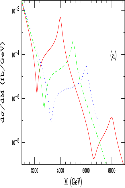
Figure 1: Cross section for Drell-Yan production of the degenerate neutral KK excitations $Z^{(n)}$ and $\gamma^{(n)}$ as a function of the dilepton invariant mass at the LHC assuming one extra dimension and naive coupling values with $1/R$=4(5, 6) TeV corresponding to the solid(dashed, dotted) curve. The second excitation is only shown for the case of $1/R=4$ TeV.

To clarify this situation let us consider the results displayed in Figs. 1 for $d=1$ where we show the production cross sections in the $\ell^{+}\ell^{-}$ channel with inverse compactification radii of 4, 5 and 6 TeV. In calculating these cross sections we have assumed that the KK excitations have their naive couplings and can only decay to the usual fermions of the SM. Additional decay modes can lead to appreciably lower cross sections so that we cannot use the peak heights to determine the degeneracy of the KK state. Note that in the 4 TeV case, which is essentially as small a mass as can be tolerated by the present data on precision measurements, the second KK excitation is visible in the plot. We see several things from these figures. First, we can easily estimate the total number of events in the resonance regions associated with each of the peaks assuming the canonical integrated luminosity of $100fb^{-1}$ appropriate for the LHC; we find $\simeq 300(32,3,0.02)$ events corresponding to the 4(5,6,8) TeV resonances if we sum over both electron and muon final states and assume $100\%$ leptonic identification efficiencies. Clearly the 6 and 8 TeV resonances will not be visible at the LHC (though a modest increase in luminosity by a factor of a few will allow the 6 TeV resonance to become visible) and we also verify our claim that only the first KK excitations will be observable. In the case of the 4 TeV resonance there is sufficient statistics that the KK mass will be well measured and one can also imagine measuring the forward-backward asymmetry, $A_{FB}$, if not the full angular distribution of the outgoing leptons, since the final state muon charges can be signed. Given sufficient statistics, a measurement of the angular distribution would demonstrate that the state is indeed spin-1 and not spin-0 or spin-2. However, for such a heavy resonance it is unlikely that much further information could be obtained about its couplings and other properties. In fact the conclusion of several years of $Z^{\prime}$ analysessnow is that coupling information will be essentially impossible to obtain for $Z^{\prime}$-like resonances with masses in excess of 1-2 TeV at the LHC due to low statistics. Furthermore, the lineshape of the 4 TeV resonance and the Drell-Yan spectrum anywhere close to the peak will be difficult to measure in detail due to both the limited statistics and energy smearing. Thus we will never know from LHC data alone whether the first KK resonance has been discovered or, instead, some extended gauge model scenario has been realized. To make further progress we need a lepton collider.

It is well-known that future $e^{+}e^{-}$ linear colliders(LC) operating in the center of mass energy range $\sqrt{s}=0.5-1.5$ TeV will be sensitive to indirect effects arising from the exchange of new $Z^{\prime}$ bosons with masses typically 6-7 times greater than $\sqrt{s}$snow . This sensitivity is even greater in the case of KK excitations since towers of both $\gamma$ and $Z$ exist all of which have couplings larger than their SM zero modes. Furthermore, analyses have shown that with enough statistics the couplings of the new $Z^{\prime}$ to the SM fermions can be extractedcoupl in a rather precise manner, especially when the $Z^{\prime}$ mass is already approximately known from elsewhere, e.g., the LHC. (If the $Z^{\prime}$ mass is not known then measurements at several distinct values of $\sqrt{s}$ can be used to extract both the mass as well as the corresponding couplingsme .) In the present situation, we imagine that the LHC has discovered and determined the mass of a $Z^{\prime}$-like resonance in the 4-6 TeV range. Can the LC tell us anything about this object?

Figure 2: Fitted values of the parameters $v_{l}$ and $a_{l}$ following the procedures described in the text for a 4 TeV KK excitation at a 500 GeV $e^{+}e^{-}$ collider. The contour described the $95\%$ CL region with the best fit value as a diamond. The normalization is such that the corresponding SM $Z$ boson’s axial-vector coupling to the electron is -1/2.

The obvious step would be to use the LC to extract the couplings of the apparent resonance discovered by the LHC; we find that it is sufficient for our arguments below to do this solely for the leptonic channels. The idea is the following: we measure the deviations in the differential cross sections and angular dependent Left-Right polarization asymmetry, $A_{LR}^{\ell}$, for the three lepton generations and combine those with $\tau$ polarization data. Assuming lepton universality(which would be observed in the LHC data anyway), that the resonance mass is well determined, and that the resonance is an ordinary $Z^{\prime}$ we perform a fit to the hypothetical $Z^{\prime}$ coupling to leptons, $v_{l},a_{l}$. To be specific, let us consider the case of only one extra dimension with a 4 TeV KK excitation and employ a $\sqrt{s}=500$ GeV collider with an integrated luminosity of 200 $fb^{-1}$. The result of performing this fit, including the effects of cuts and initial state radiation, is shown in Fig.2. Here we see that the coupling values are ‘well determined’ (i.e., the size of the $95\%$ CL allowed region we find is quite small) by the fitting procedure as we would have expected from previous analyses of $Z^{\prime}$ couplings extractions at linear colliderssnow ; coupl ; me .

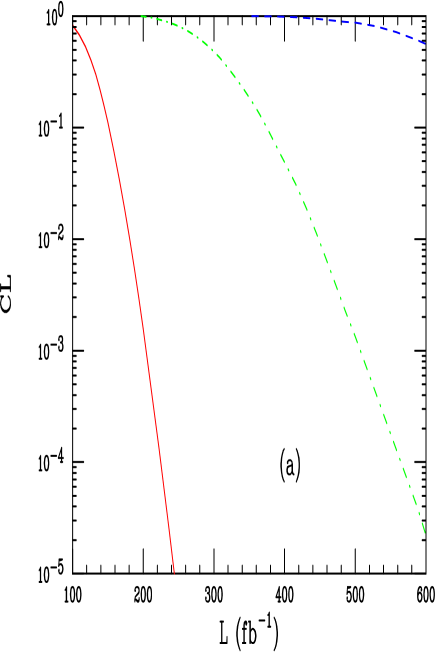
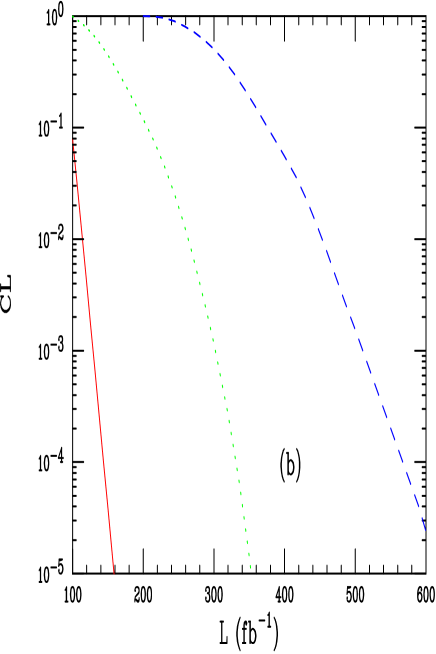
Figure 3: CL as a function of the integrated luminosity resulting from the coupling fits following from the analysis discussed in the text for both (a) a 500 GeV or a (b) 1 TeV $e^{+}e^{-}$ collider. In (a) the solid(dash-dotted,dotted) curve corresponds to a first KK excitation mass of 4(5,6) TeV. In (b) the solid(dotted,dashed) curve corresponds to a first KK mass of 5(6,7) TeV.

The only problem with the fit shown in the figure is that the $\chi^{2}$ is very large leading to a very small confidence level, i.e., $\chi^{2}/d.o.f=95.06/58$ or CL=$1.55\times 10^{-3}$! (We note that this result is not very sensitive to the assumption of $90\%$ beam polarization; $70\%$ polarization leads to almost identical results.) For an ordinary $Z^{\prime}$ it has been shown that fits of much higher quality, based on confidence level values, are obtained by this same procedure. Increasing the integrated luminosity can be seen to only make matters worse. Fig.3 shows the results for the CL following the above approach as we vary both the luminosity and the mass of the first KK excitation at both 500 GeV and 1 TeV $e^{+}e^{-}$ linear colliders. From this figure we see that the resulting CL is below $\simeq 10^{-3}$ for a first KK excitation with a mass of 4(5,6) TeV when the integrated luminosity at the 500 GeV collider is 200(500,900)$fb^{-1}$ whereas at a 1 TeV for excitation masses of 5(6,7) TeV we require luminosities of 150(300,500)$fb^{-1}$ to realize this same CL. Barring some unknown systematic effect the only conclusion that one could draw from such bad fits is that the hypothesis of a single $Z^{\prime}$, and the existence of no other new physics, is simply wrong. If no other exotic states are observed below the first KK mass at the LHC, such as $\tilde{\nu}$rp or leptoquarksleptos , this result would give very strong indirect evidence that something more unusual that a conventional $Z^{\prime}$ had been found but cannot prove that this is a KK state.

SM KK States at Muon Colliders

In order to be completely sure of the nature of the first KK excitation, we must produce it directly at a higher energy lepton collider and sit on and near the peak of the KK resonance. To reach this mass range will most likely require a Muon Collider. The first issue to address is the quality of the degeneracy of the $\gamma^{(1)}$ and $Z^{(1)}$ states. Based on the analyses in Ref.host ; rw we can get an idea of the maximum possible size of this fractional mass shift and we find it to be of order $\sim M_{Z}^{4}/M_{Z^{(1)}}^{4}$, an infinitesimal quantity for KK masses in the several TeV range. Thus even when mixing is included we find that the $\gamma^{(1)}$ and $Z^{(1)}$ states remain very highly degenerate so that even detailed lineshape measurements may not be able to distinguish the $\gamma^{(1)}/Z^{(1)}$ composite state from that of a $Z^{\prime}$. We thus must turn to other parameters in order to separate these two cases.

Sitting on the resonance there are a very large number of quantities that can be measured: the mass and apparent total width, the peak cross section, various partial widths and asymmetries etc. From the $Z$-pole studies at SLC and LEP, we recall a few important tree-level results which we would expect to apply here as well provided our resonance is a simple $Z^{\prime}$. First, we know that the value of $A_{LR}=[A_{e}=2v_{e}a_{e}/(v_{e}^{2}+a_{e}^{2})]$, as measured on the $Z$ by SLD, does not depend on the fermion flavor of the final state and second, that the relationship $A_{LR}\cdot A_{FB}^{pol}(f)=A_{FB}^{f}$ holds, where $A_{FB}^{pol}(f)$ is the polarized Forward-Backward asymmetry as measured for the $Z$ at SLC and $A_{FB}^{f}$ is the usual Forward-Backward asymmetry. The above relation is seen to be trivially satisfied on the $Z$(or on a $Z^{\prime}$) since $A_{FB}^{pol}(f)={3\over 4}A_{f}$ and $A_{FB}^{f}={3\over 4}A_{e}A_{f}$. Both of these relations are easily shown to fail in the present case of a ‘dual’ resonance though they will hold if only one particle is resonating.

A short exercise shows that in terms of the couplings to $\gamma^{(1)}$, which we will call $v_{1},a_{1}$, and $Z^{(1)}$, now called $v_{2},a_{2}$, these same observables can be written as

$$A_{FB}^{f} = {3\over 4}{A_{1}\over D}$$

$$A_{FB}^{pol}(f) = {3\over 4}{A_{2}\over D}$$

$$A_{LR}^{f} = {A_{3}\over D}\,,$$ (2)

where $f$ labels the final state fermion and we have defined the coupling combinations

$$D = (v_{1}^{2}+a_{1}^{2})_{e}(v_{1}^{2}+a_{1}^{2})_{f}+R^{2}(v_{2}^{2}+a_{2}^{2})_{e}(v_{2}^{2}+a_{2}^{2})_{f}$$ (3)

$$\quad+2R(v_{1}v_{2}+a_{1}a_{2})_{e}(v_{1}v_{2}+a_{1}a_{2})_{f}$$

$$A_{1} = (2v_{1}a_{1})_{e}(2v_{1}a_{1})_{f}+R^{2}(2v_{2}a_{2})_{e}(2v_{2}a_{2})_{f}+2R(v_{1}a_{2}+v_{2}a_{1})_{e}(v_{1}a_{2}+v_{2}a_{1})_{e}$$

$$A_{2} = (2v_{1}a_{1})_{f}(v_{1}^{2}+a_{1}^{2})_{e}+R^{2}(2v_{2}a_{2})_{f}(v_{2}^{2}+a_{2}^{2})_{e}+2R(v_{1}a_{2}+v_{2}a_{1})_{f}(v_{1}v_{2}+a_{1}a_{2})_{e}$$

$$A_{3} = (2v_{1}a_{1})_{e}(v_{1}^{2}+a_{1}^{2})_{f}+R^{2}(2v_{2}a_{2})_{e}(v_{2}^{2}+a_{2}^{2})_{f}+2R(v_{1}a_{2}+v_{2}a_{1})_{e}(v_{1}v_{2}+a_{1}a_{2})_{f}\,,$$

with $R$ being the ratio of the widths of the two KK states, $R=\Gamma_{1}/\Gamma_{2}$, and the $v_{1,2i},a_{1,2i}$ are the appropriate couplings for electrons and fermions $f$. Note that when $R$ gets either very large or very small we recover the usual ‘single resonance’ results. Examining these equations we immediately note that $A_{LR}^{f}$ is now flavor dependent and that the relationship between observables is no longer satisfied:

$$A_{LR}^{f}\cdot A_{FB}^{pol}(f)\neq A_{FB}^{f}\,,$$ (4)

which clearly tells us that we are actually producing more than one resonance.

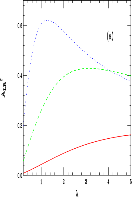
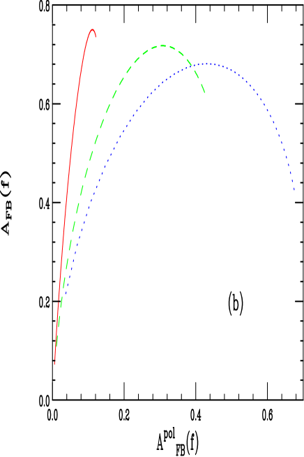
Figure 4: (a) $A_{LR}^{f}$ as a function of the parameter $\lambda$ for $f=\ell$(solid), $f=c$(dashed) and $f=b$(dots). (b) Correlations between on-peak observables for the same three cases as shown in (a). $\lambda$ varies from 0.2 to 5 along each curve.

Of course we need to verify that these single resonance relations are numerically badly broken before clear experimental signals for more than one resonance can be claimed. Statistics will not be a problem with any reasonable integrated luminosity since we are sitting on a resonance peak and certainly millions of events will be collected. With such large statistics only a small amount of beam polarization will be needed to obtain useful asymmetries. In principle, to be as model independent as possible in a numerical analysis, we should allow the widths $\Gamma_{i}$ to be greater than or equal to their SM values as such heavy KK states may decay to SM SUSY partners as well as to presently unknown exotic states. Since the expressions above only depend upon the ratio of widths, we let $R=\lambda R_{0}$ where $R_{0}$ is the value obtained assuming that the KK states have only SM decay modes. We then treat $\lambda$ as a free parameter in what follows and explore the range $1/5\leq\lambda\leq 5$. Note that as we take $\lambda\rightarrow 0(\infty)$ we recover the limit corresponding to just a $\gamma^{(1)}(Z^{(1)})$ being present.

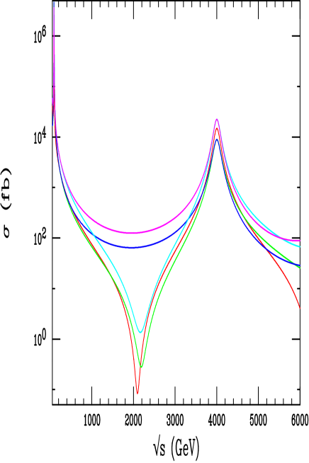
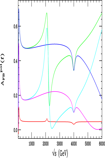
Figure 5: Cross sections and polarized $A_{FB}$ for $\mu^{+}\mu^{-}\rightarrow e^{+}e^{-}$ $b\bar{b}$ and $c\bar{c}$ as functions of energy in both the ‘conventional’ scenario and that of Arkani-Hamed and Schmaltz(AS)schm where the quarks and leptons are separated in the extra dimension by a distance $D=\pi R$. The red curve applies for the $\mu$ final state in either model whereas the green(blue) and cyan(magenta) curves label the $b$ and $c$ final states for the ‘conventional’(AS) scenario.

In Fig.4 we display the flavor dependence of $A_{LR}^{f}$ as a functions of $\lambda$. Note that as $\lambda\rightarrow 0$ the asymmetries vanish since the $\gamma^{(1)}$ has only vector-like couplings. In the opposite limit, for extremely large $\lambda$, the $Z^{(1)}$ couplings dominate and a common value of $A_{LR}$ will be obtained. It is quite clear, however, that over the range of reasonable values of $\lambda$, $A_{LR}^{f}$ is quite obviously flavor dependent. We also show in Fig.4 the correlations between the observables $A_{FB}^{pol}(f)$ and $A_{FB}(f)$ which would be flavor independent if only a single resonance were present. From the figure we see that this is clearly not the case. Note that although $\lambda$ is an a priori unknown parameter, once any one of the electroweak observables are measured the value of $\lambda$ will be directly determined. Once $\lambda$ is fixed, then the values of all of the other asymmetries, as well as the ratios of various partial decay widths, are all completely fixed for the KK resonance with uniquely predicted values. This means that we can directly test the couplings of this apparent single resonance against what might be expected for a degenerate pair of KK excitations without any ambiguities.

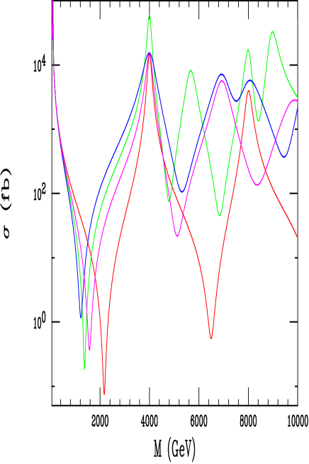
Figure 6: Same as Fig. 5a for the process $\mu^{+}\mu^{-}\rightarrow e^{+}e^{-}$ but now also including the models listed in Table 1 with $d=2$ assuming $M_{1}=4$ TeV. The red(green,blue,purple) curve corresponds to the $S^{1}/Z_{2}$($Z_{2}\times Z_{2}$, $Z_{3,6}$, $S^{2}$) compactifications.

In Figs. 5a and 5b we show that although on-resonance measurements of the electroweak observables, being quadratic in the $Z^{(1)}$ and $\gamma^{(1)}$ couplings, will not distinguish between the usual KK scenario and that of the Arkani-Hamed and Schmaltz(AS) (whose KK couplings to quarks are of opposite sign from the conventional assignments for odd KK levels since quarks and leptons are assumed to be separated by a distance $D=\pi R$ in their scenario) the data below the peak in the hadronic channel will easily allow such a separation. The cross section and asymmetries for $\mu^{+}\mu^{-}\rightarrow e^{+}e^{-}$ (or vice versa) is, of course, the same in both cases. Such data can be collected by using radiative returns if sufficient luminosity is available. The combination of on and near resonance measurements will thus completely determine the nature of the resonance.

We note that all of the above analysis will go through essentially unchanged in any qualitative way when we consider the case of the first KK excitation in a theory with more than one extra dimension as is shown in Fig.6. Here we see that the shape of the excitation curves for the $d=1$ case and the $d>1$ models listed in Table 1 will clearly allow the number of dimensions and the compactification scheme to be uniquely identified.

Randall-Sundrum Gravitons at Muon Colliders

The possibility of extra space-like dimensions with accessible physics near the TeV scale has recently opened a new window on the possible solutions to the hierarchy problem. Models designed to address this problem make use of our ignorance about gravity, in particular, the fact that gravity has yet to be probed at energy scales much above $10^{-3}$ eV in laboratory experiments. The prototype scenario in this class of theories is due to Arkani-Hamed, Dimopoulos and Dvali(ADD)nima who use the volume associated with large extra dimensions to bring the $d$-dimensional Planck scale down to a few TeV. Here the hierarchy problem is recast into trying to understand the rather large ratio of the TeV Planck scale to the size of the extra dimensions which may be as large as a fraction of a millimeter. The phenomenologicalpheno implications of this model have been worked out by a large number of authors. An extrapolation of these analyses to the case of high energy muon colliders shows an enormous reach for this kind of physics.

More recently, Randall and Sundrum(RS)rs have proposed a new scenario wherein the hierarchy is generated by an exponential function of the compactification radius, called a warp factor. Unlike the ADD model, they assume a 5-dimensional non-factorizable geometry, based on a slice of $AdS_{5}$ spacetime. Two 3-branes, one being ‘visible’ with the other being ‘hidden’, with opposite tensions rigidly reside at $S_{1}/Z_{2}$ orbifold fixed points, taken to be $\phi=0,\pi$, where $\phi$ is the angular coordinate parameterizing the extra dimension. It is assumed that the extra-dimension bulk is only populated by gravity and that the SM lies on the brane with negative tension. The solution to Einstein’s equations for this configuration, maintaining 4-dimensional Poincare invariance, is given by the 5-dimensional metric

$$ds^{2}=e^{-2\sigma(\phi)}\eta_{\mu\nu}dx^{\mu}dx^{\nu}+r_{c}^{2}d\phi^{2}\,,$$ (5)

where the Greek indices run over ordinary 4-dimensional spacetime, $\sigma(\phi)=kr_{c}|\phi|$ with $r_{c}$ being the compactification radius of the extra dimension, and $0\leq|\phi|\leq\pi$. Here $k$ is a scale of order the Planck mass and relates the 5-dimensional Planck scale $M$ to the cosmological constant. Examination of the action in the 4-dimensional effective theory in the RS scenario yields the relationship $\overline{M}_{Pl}^{2}=M^{3}/k$ for the reduced effective 4-D Planck scale.

Assuming that we live on the 3-brane located at $|\phi|=\pi$, it is found that a field on this brane with the fundamental mass parameter $m_{0}$ will appear to have the physical mass $m=e^{-kr_{c}\pi}m_{0}$. TeV scales are thus generated from fundamental scales of order $\overline{M}_{Pl}$ via a geometrical exponential factor and the observed scale hierarchy is reproduced if $kr_{c}\simeq 11-12$. Hence, due to the exponential nature of the warp factor, no additional large hierarchies are generated.

A recent analysisdhr examined the phenomenological implications and constraints on the RS model that arise from the exchange of weak scale towers of gravitons. There it was shown that the masses of the KK graviton states are given by $m_{n}=kx_{n}e^{-kr_{c}\pi}$ where $x_{n}$ are the roots of $J_{1}(x_{n})=0$, the ordinary Bessel function of order 1. It is important to note that these roots are not equally spaced, in contrast to most KK models with one extra dimension, due to the non-factorizable metric. Expanding the graviton field into the KK states one finds the interaction

$${\cal L}=-{1\over\overline{M}_{Pl}}T^{\alpha\beta}(x)h^{(0)}_{\alpha\beta}(x)-{1\over\Lambda_{\pi}}T^{\alpha\beta}(x)\sum_{n=1}^{\infty}h^{(n)}_{\alpha\beta}(x)\,.$$ (6)

Here, $T^{\alpha\beta}$ is the stress energy tensor on the brane and we see that the zero mode separates from the sum and couples with the usual 4-dimensional strength, $\overline{M}_{Pl}^{-1}$; however, all the massive KK states are only suppressed by $\Lambda_{\pi}^{-1}$, where we find that $\Lambda_{\pi}=e^{-kr_{c}\pi}\overline{M}_{Pl}$, which is of order the weak scale.

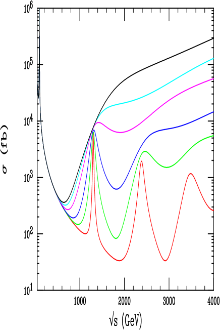
Figure 7: Cross section for $\mu^{+}\mu^{-}\rightarrow e^{+}e^{-}$ including the exchange of KK gravitons, taking the mass of the first mode to be 1.2 TeV, as a function of energy. From top to bottom the curves correspond to c=1.0, 0.7, 0.5, 0.3, 0.2, and 0.1.

This model has essentially 2 free parameters which we can take to be the mass of the first KK graviton mode and the ratio $c=k/\overline{M}_{Pl}$; the later quantity is restricted to be less than unity to maintain the self-consistency of the scenario (to prevent a radius of curvature smaller than the Planck scale in 5 dimensions) and if it is taken too small another hierarchy is formed. Figs.7 and 8 show the cross section and $A_{FB}$ for the process $\mu^{+}\mu^{-}\rightarrow e^{+}e^{-}$ as a function of $\sqrt{s}$ in the presence of KK graviton resonances for several values of the parameter $c$. For large $c$ one does not see the individual resonance structures (since the theory is strongly coupled and they are smeared together by their large widths which grow as $\sim c^{2}$) but only a very large shoulder somewhat similar to a contact interaction. For small $c$ one sees the individual resonances with their widths growing rapidly with increasing mass as $\sim m_{n}^{3}$. Note that for large $\sqrt{s}$ where graviton exchange dominates the value of $A_{FB}$ is driven to zero. Sitting on any of these KK resonances, in the case of small values of $c$, will immediately reveal the unique quartic angular distribution corresponding to spin-2 graviton exchange for the fermions in the final state $\sim 1-3\cos^{2}\theta+4\cos^{4}\theta$.

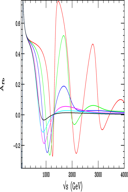
Figure 8: Same as the previous figure but now for the Forward-Backward asymmetry in the RS model. The color code is as in the previous figure.

Conclusions

Present data indicates that the masses of KK excitations of the SM gauge bosons must be rather heavy, e.g., $>3.9$ TeV if $d=1$. We have found that:

• With an integrated luminosity of $100~{}fb^{-1}$, the LHC will be able to observe KK excitations in the mass range below $\simeq 6$ TeV but may not see any KK excitations when $d>1$ since they are likely to be more massive. The LHC will not see the second set of KK resonances even when $d=1$.

• The LHC cannot separate the KK states $\gamma^{(1)}$ from $Z^{(1)}$ which will appear together as a single resonance, nor can it obtain significant coupling constant information.

• The LHC cannot see the $g^{(1)}$ if its mass is in excess of $\sim 4$ TeV due to its large width and the energy resolution of the LHC detectors.

• The LHC cannot distinguish an extended electroweak model with a degenerate $Z^{\prime}/W^{\prime}$ from a KK scenario. All we will know is the mass of these resonances.

• A LC with $\sqrt{s}=0.5-1$ TeV will be sensitive to the existence of KK states with masses more than an order of magnitude larger than $\sqrt{s}$ for reasonable integrated luminosities $\simeq 100~{}fb^{-1}$.

• At a LC, the extraction of the couplings of an apparent $Z^{\prime}$, whose mass is known from measurements obtained at the LHC, can be performed in a straightforward manner with reasonable integrated luminosities. However, the $Z^{\prime}$ hypothesis will yield a poor fit to the data if the state in question is actually the combined $\gamma^{(1)}/Z^{(1)}$ KK excitation. The LC will not be able to identify this state as such–only prove it is not a $Z^{\prime}$.

• A Muon Collider operating at or above the first KK resonance pole will identify it as a KK state provided polarized beams are available.

• Measurements of the KK excitation spectrum at Muon Colliders will be able to tell us both the number of extra dimensions and how they are compactified thus possibly revealing the basic underlying theory upon which the KK scenario is based.

• KK excitations of gravitons in the RS model can be studied in detail at both LC and Muon Colliders with Muon Colliders providing a much larger reach in explorable parameter space. These measurements can completely determine all of the parameters of this model.

Muon Colliders clearly offer a very important window into the physics of Kaluza-Klein excitations.

References

- (1) I. Antoniadis, Phys. Lett. B246, 377 (1990); I. Antoniadis, C. Munoz and M. Quiros, Nucl. Phys. B397, 515 (1993); I. Antoniadis and K. Benalki, Phys. Lett. B326, 69 (1994); I. Antoniadis, K. Benalki and M. Quiros, Phys. Lett. B331, 313 (1994).
- (2) D0 Collaboration, S. Abachi et al.,Phys. Lett. B385, 471 (1996), Phys. Rev. Lett. 76, 3271 (1996) and Phys. Rev. Lett. 82, 29 (1999); CDF Collaboration, F. Abe et al., Phys. Rev. Lett. 77, 5336 (1996), Phys. Rev. Lett. 74, 2900 (1995) and Phys. Rev. Lett. 79, 2191 (1997).
- (3) F. Cornet, M. Relano and J. Rico, hep-ph/9908299.
- (4) P. Nath and M. Yamaguchi, hep-ph/9902323 and hep-ph/9903298; M. Masip and A. Pomarol, hep-ph/9902467; W.J. Marciano, hep-ph/9903451; L. Hall and C. Kolda, Phys. Lett. B459, 213 (1999); R. Casalbuoni, S. DeCurtis and D. Dominici, hep-ph/9905568; R. Casalbuoni, S. DeCurtis, D. Dominici and R. Gatto, hep-ph/9907355; A. Strumia, hep-ph/9906266; C.D. Carone, hep-ph/9907362.
- (5) T.G. Rizzo and J.D. Wells, hep-ph/9906234.
- (6) J. Mnich, talk given at the International Europhysics Conference on High Energy Physics(EPS99), 15-21 July 1999, Tampere, Finland; M. Swartz, M. Lancaster and D. Charlton talks given at the XIX International Symposium on Lepton and Photon Interactions, 9-14 August 1999, Stanford, California.
- (7) T.G. Rizzo, hep-ph/9909232; See also I. Antoniadis, K. Benalki and M. Quiros, hep-ph/9905311; P. Nath, Y. Yamada and M. Yamaguchi, hep-ph/9905415.
- (8) M. Bando, T. Kugo, T. Noguchi and K. Yoshioka, hep-ph/9906549. See also J. Hisano and N. Okada, hep-ph/9909555.
- (9) N. Arkani-Hamed and M. Schmaltz, hep-ph/9903417; N. Arkani-Hamed, Y. Grossman and M. Schmaltz, hep-ph/9909411.
- (10) For a discussion of a few of these models, see H. Georgi, E.E. Jenkins, and E.H. Simmons, Phys. Rev. Lett. 62, 2789 (1989) and Nucl. Phys. B331, 541 (1990);V. Barger and T.G. Rizzo, Phys. Rev. D41, 946 (1990); T.G. Rizzo, Int. J. Mod. Phys. A7, 91 (1992); R.S. Chivukula, E.H. Simmons and J. Terning, Phys. Lett. B346, 284 (1995); A. Bagneid, T.K. Kuo, and N. Nakagawa, Int. J. Mod. Phys. A2, 1327 (1987) and Int. J. Mod. Phys. A2, 1351 (1987); D.J. Muller and S. Nandi, Phys. Lett. B383, 345 (1996); X.Li and E. Ma, Phys. Rev. Lett. 47, 1788 (1981) and Phys. Rev. D46, 1905 (1992); E. Malkawi, T.Tait and C.-P. Yuan, Phys. Lett. B385, 304 (1996); E. Malkawi and C.-P. Yuan, hep-ph/9906215.
- (11) For a review of new gauge boson physics at colliders and details of the various models, see J.L. Hewett and T.G. Rizzo, Phys. Rep. 183, 193 (1989); M. Cvetic and S. Godfrey, in Electroweak Symmetry Breaking and Beyond the Standard Model, ed. T. Barklow et al., (World Scientific, Singapore, 1995), hep-ph/9504216; T.G. Rizzo in New Directions for High Energy Physics: Snowmass 1996, ed. D.G. Cassel, L. Trindle Gennari and R.H. Siemann, (SLAC, 1997), hep-ph/9612440; A. Leike, hep-ph/9805494.
- (12) A. Djouadi, A. Lieke, T. Riemann, D. Schaile and C. Verzegnassi, Z. Phys. C56, 289 (1992); J. Hewett and T. Rizzo, in Proceedings of the Workshop on Physics and Experiments with Linear Colliders, September 1991, Saariselkä, Finland, R. Orava ed., (World Scientific, Singapore, 1992) Vol. II, p.489, ibid p.501; G. Montagna et al., Z. Phys. C75, 641 (1997); F. del Aguila and M. Cvetic, Phys. Rev. D50, 3158 (1994); F. del Aguila, M. Cvetic and P. Langacker Phys. Rev. D52, 37 (1995); A. Lieke, Z. Phys. C62, 265 (1994); D. Choudhury, F. Cuypers and A. Lieke, Phys. Lett. B333, 531 (1994); S. Riemann in New Directions for High Energy Physics: Snowmass 1996, ed. D.G. Cassel, L. Trindle Gennari and R.H. Siemann, (SLAC, 1997), hep-ph/9610513; A. Lieke and S. Riemann, Z. Phys. C75, 341 (1997); T.G. Rizzo, hep-ph/9604420.
- (13) T.G. Rizzo, Phys. Rev. D55, 5483 (1997).
- (14) T.G. Rizzo, Phys. Rev. D59, 113004 (1999).
- (15) For a review, see J.L. Hewett and T.G. Rizzo, Phys. Rev. D56, 5709 (1997) and Phys. Rev. D58, 055005 (1998).
- (16) N. Arkani-Hamed, S. Dimopoulos and G. Dvali, Phys. Lett. B429, 263 (1998) and Phys. Rev. D59, 086004 (1999); I. Antoniadis, N. Arkani-Hamed, S. Dimopoulos and G. Dvali, Phys. Lett. B436, 257 (1998.)
- (17) G.F. Giudice, R. Rattazzi and J.D. Wells, Nucl. Phys. B544, 3 (1999); E.A. Mirabelli, M. Perelstein and M.E. Peskin, Phys. Rev. Lett. 82, 2236 (1999); T. Han, J.D. Lykken and R. Zhang, Phys. Rev. D59, 105006 (1999); J.L. Hewett, Phys. Rev. Lett. 82, 4765 (1999); T.G. Rizzo, Phys. Rev. D59, 115010 (1999).
- (18) L. Randall and R. Sundrum, hep-ph/9905221 and hep-th/9906182.
- (19) H. Davoudiasl, J.L. Hewett and T.G. Rizzo, hep-ph/9909255.