A Tale of Two Hard Pomerons

Abstract

Two mechanisms are examined for hard double pomeron exchange dijet production, the factorized model of Ingelman-Schlein and the nonfactorized model of lossless jet production which exhibits the Collins-Frankfurt-Strikman mechanism. Comparison between these two mechanisms are made of the total cross section, $E_{T}$-spectra, and mean rapidity spectra. For both mechanisms, several specific models are examined with the cuts of CDF, DØ  and representative cuts of LHC. Distinct qualitative differences are predicted by the two mechanisms for the CDF $y_{+}$-spectra and for the $E_{T}$-spectra for all three experimental cuts. The preliminary CDF and DØ experimental data for this process are interpreted in terms of these two mechanisms. The $y_{+}$-spectra of the CDF data is suggestive of domination by the factorized Ingelman-Schlein mechanism, whereas the DØ data shows no greater preference for either mechanism. An inconsistency is found amongst all the theoretical models in attempting to explain the ratio of the cross sections given by the data from these two experiments.

PACS number(s): 13.85.-t, 12.38.Qk, 13.87.Ce

hep-ph/9910405

In press Physical Review D, 2000

I Introduction

In diffractive hard scattering, the incident hadron in e-p collisions and one or both hadrons in ${\bar{p}}p$ collisions participate in a hard interaction involving very large momentum transfer, but nevertheless the respective hadrons emerge with small transverse momenta and a loss of small fractions of their longitudinal momenta. For such diffractive hard processes, first comes a question of pure semantics, whether or not to say the diffractive proton ”exchanged a pomeron”. Only one Pomeron has entitled historical rights to this name, and that is the Pomeron of soft Regge physics [1, 2] (also sometimes called the soft Pomeron). Reference to pomeron in any other case exploits this established trademark as a mnemonic for describing some portion of the process in which a strong interaction scattering occurred that involved the exchange of no quantum numbers except angular momentum. In our discussion of diffractive hard scattering, we will use the lower case pomeron in reference to a process in which one or both incoming hadrons diffracts into the final state along with a hard process. On the other hand, the upper case Pomeron will be reserved for the vacuum exchange trajectory of soft Regge physics [1, 2].

There is general belief that properties of the Pomeron reflect in the pomeron of diffractive hard scattering, although it is a central research question to identify the specifics. Spacetime arguments generically suggest that hard events are well localized in space and time. Thus it is expected that in a diffractive hard process, the diffractive hadrons undergo effects similar to what they would encounter in a high-energy elastic scattering. As such, diffractive hard physics is expected to involve long-time, long distance, thus nonperturbative, physics. Nevertheless, that hard processes can occur intermittent to the diffractive scattering indicates that diffractive hadronic physics, via the pomeron, also possesses perturbative properties that can be explained through perturbative QCD.

A primary goal of diffractive hard scattering physics is to unify the QCD picture of the pomeron with the phenomenological Regge physics description (for a review of Regge phenomenology applied to diffractive physics please see [3, 4]). Hard double pomeron exchange (DPE) processes are useful in addressing this question, since it turns out the QCD and Regge physics description of these processes have some distinct qualitative differences, which are best expressed in the context of hard factorization.

Recall, for a hard scattering factorized process, the effect of the two incoming particles act independently on the hard event [5, 6]. The basic Regge physics motivated model of hard diffractive processes is the Ingelman-Schlein model [7], and this model assumes hard factorization. In their model, diffractive scattering is attributed to the exchange of a pomeron, which operationally is defined as a colorless object with vacuum quantum numbers. Their model treats the pomeron like a real particle and so considers, for example, that a diffractive electron-proton collision is due to an electron-pomeron collision and that a diffractive hadron-hadron collision is due to a proton-pomeron collision for single-sided diffraction and pomeron-pomeron collision for double diffraction.

For diffractive deep inelastic scattering, basic ideas of hard factorization were outlined and diffractive parton distribution functions were defined in [12, 13]. A proof of factorization for diffractive DIS was given in [15]. For hard diffraction in pure hadronic collisions, Collins, Frankfurt and Strikman (CFS) [16] have demonstrated a counterargument to hard factorization. The CFS mechanism is a leading twist effect in which all the momentum lost by the diffractive hadrons goes into the hard event. An important feature about the CFS mechanism is that it requires the color flow properties of QCD in an essential way. In general, the presence of color in QCD implies pomeron exchange in simplest form is a two gluon exchange process [17, 18]. Necessarily, the simplest model of the pomeron must involve at least two partons in order to be color singlet. The two gluon pomeron model has a key property for any pure hadron initiated reaction, which is a realization of the CFS mechanism. Consider the hard DPE process $h_{1}h_{2}\rightarrow h_{1}h_{2}+hard$, where $h_{1},h_{2}$ are the colliding hadrons. The two gluons exchanged by $h_{1}$ are not both obliged to enter the hard event. Instead, one gluon may attach to $h_{2}$. In this case, the two incoming hadrons no longer act independently in inducing the hard event. By definition of hard factorization [5, 6], such a process is nonfactorizing.

This mechanism was identified earlier by Frankfurt and Strikman [19]. They originally referred to the nonfactorized pomeron of CFS as the coherent pomeron. Subsequently, the UA8 presented results [20] in which up to 30 percent of the dijet events in single-sided diffraction could be associated with the coherent pomeron, which they in turn named the superhard pomeron. With the hindsight of the UA8 experiment and the ideas of CFS, in [12] the CFS mechanism was applied to a toy quantum field theory model of diffractive dijet photoproduction, in which the pomeron was represented by two gluon exchange. This work in turn, in turn, named the nonfactorizing, alias superhard, alias coherent pomeron process as lossless diffractive hard scattering to emphasize the efficient transfer of the pomeron momentum to the hard process.

The CFS mechanism has been developed for hard DPE in ${\bar{p}}p$ collisions for quark jets in [21] and gluon jets in [22]. The gluon jet process was shown in [22] to dominate the quark jet process by several orders of magnitude.

The purpose of this paper is to examine for the DPE dijet process, general differences between the factorized pomeron model of Ingelman and Schlein, F(IS)DPE [7], and the nonfactorized pomeron model of lossless jet production of Berera and Collins [22], N(L)DPE. Our notation specifies in the context of hard factorization whether the process is factorizable, F, or nonfactorizable, N, and in parenthesis gives the particular type of process. The latter specification is necessary since there are several different types of factorizable and nonfactorizable processes. Detailed discussions about this point are in [16, 12, 13, 22, 15, 25, 26]. As one example, factorized processes first have a basic distinction between simple hard factorization and the more specific Regge factorization [13]. In particular, the factorized Ingelman-Schlein DPE model also is Regge factorized.

For nonfactorization, one example outside of the CFS mechanism is the ”flux renormalization” prescription of Goulianos [27], which arises due to a breakdown of the triple-Regge theory for soft diffractive excitation. Also, nonfactorization is found in pre-QCD analysis of diffractive processes [28]. An empirical analysis by Alvero, Collins and Whitmore [29] of the preliminary CDF double diffractive dijet data [30, 31] indicates that hard factorization is violated in this process. In fact, their analysis suggests for parton distribution functions that are most consistent over all diffractive processes, the experimental DPE dijet cross section is much less than expected by factorization. On the other hand, the nonfactorizing CFS mechanism should enhance the cross section. Nevertheless, the analysis in [29] does not rule-out experimental realization of the CFS mechanism, since general understanding from Regge models suggests that there is a large source of suppression which will emerge from effects generically termed absorptive corrections. These effect are due to exchanges of pomerons and gluons between particles in the basic model that possess very different rapidities, thus in particular between the two incoming hadrons. As such, these effects also are nonfactorizing. Actual computation of absorptive corrections is nontrivial since they are nonperturbative. Some work has been done to estimate their effects [32, 33]. A general conclusion of these works is that absorptive correction effects are independent of the hard kinematics and weakly s-dependent. As such, these effects should be very easy to distinguish from the N(L)DPE process. Also, these effects only should shift, in particular decrease, the values of the cross sections from those computed in our basic models and the effect should be the same for either the F(IS)DPE or N(L)DPE processes. In this paper, we are interested in examining qualitative differences between the F(IS)DPE and N(L)DPE processes, which are minimally model dependent. For this we will examine the $E_{T}$ and mean rapidity ($y_{+}$) spectra for both processes and for the cuts of CDF, DØ and representative cuts for LHC. We also will present total cross sections for all the models and all the experimental cuts. Thus the interested reader can test any suppression factor from any absorptive correction model that they wish.

The reason that we do not give a demonstrative example of the overall absorptive correction suppression factor is that, as will be seen in the sequal, for all the models that are examined, we find disagreement in the ratios of the cross sections from those found in the available experimental data. This discrepancy minimally is of order $\sim 5$. Present understanding about absorptive corrections can not explain this discrepancy, since their effect only is to shift the cross sections by the same overall correction factor which drops out in the ratios. This discrepancy may reflect upon a limitation of our partonic level calculations or other controllable theoretical sources, or it may be that since the experimental data is still preliminary, it may yet be modified. We will not attempt to formulate any theoretical explanations for this discrepancy found in this paper. Our modest goal is to examine the predictions of the basic models, which up to now still have not adequately been done for these processes. Of special interest is to identify features that are minimally model dependent. Furthermore, in light of the breakdown of hard factorization suggested in [29], it is important to know whether any features of the basic models are seem in the data.

The paper is organized as follows. Sect. II reviews the kinematics of DPE dijet production and then models are presented for the nonfactorized and factorized processes. The inclusive dijet cross section also is reviewed in Sect. II and will be computed in later sections for comparison purposes. In Sect. III the CDF and DØ cuts for DPE dijet production are reviewed and representatives cuts for LHC are presented. In Sect. IV results of our calculations are presented for DPE and inclusive dijet $E_{T}$ and mean rapidity spectra and total cross sections. Subsect. IV A gives a general presentation of the results, Subsect. IV B examines the results in greater detail and Subsect. IV C compares our results with the preliminary data of CDF and DØ . Finally Sect. V presents our conclusions. Also in the last part of Sect. V, we discuss limitations of our models and compare with related models. Subsects. IV B and IV C present our results with considerable detail. For readers not wishing this much detail, the first part of Sect. V concisely summarizes the basic results before proceeding to give our conclusions about them.

II Models

This section reviews the kinematics of DPE dijet production and the formulas for the F(IS)DPE and N(L)DPE models, based on the presentation in [22].

A Kinematics

The DPE dijet process examined in this paper is shown in Fig. 1,

$$p+{\bar{p}}\rightarrow p^{\prime}+{\bar{p}}^{\prime}+\mbox{\rm 2 jets}.$$ (1)

The proton and antiproton collide at high center of mass energy $s\equiv(P_{p}+P_{\bar{p}})^{2}\rightarrow\infty$, lose tiny fractions $x_{{IP}/p}$ and $x_{{IP}/{\bar{p}}}$ of their respective longitudinal momenta, and acquire transverse momenta ${\bf Q}_{p}$ and ${\bf Q}_{\bar{p}}$. (This defines a diffractive regime, and in Regge theory would lead to an expectation of the dominance of double pomeron exchange (DPE)). Using light-cone coordinates $(+,-;{\bf\perp})$, the components of momenta of the hadrons in Fig. 1 are

$$P_{p} = \left(\sqrt{\frac{s}{2}},\frac{M^{2}}{\sqrt{2s}};{\bf 0}\right)$$ (2)

$$P_{{\bar{p}}} = \left(\frac{M^{2}}{\sqrt{2s}},\sqrt{\frac{s}{2}};{\bf 0}\right)$$ (3)

$$P_{p^{\prime}} = \left((1-x_{{IP}/p})\sqrt{\frac{s}{2}},\frac{(M^{2}+{\bf Q}_{p}^{2})}{(1-x_{{IP}/p})\sqrt{2s}};{\bf Q}_{p}\right)$$ (4)

$$P_{{\bar{p}}^{\prime}} = \left(\frac{(M^{2}+{\bf Q}_{\bar{p}}^{2})}{(1-x_{{IP}/{\bar{p}}})\sqrt{2s}},(1-x_{{IP}/{\bar{p}}})\sqrt{\frac{s}{2}};{\bf Q}_{\bar{p}}\right).$$ (5)

Here we use bold-face type to indicate two-dimensional transverse momentum.

The jets carry large momenta of magnitude $E_{T}$ in the plane perpendicular to the collision axis with azimuthal angle $\phi$. (This defines a hard-scattering regime.) The small transfer of longitudinal momentum to the hard process implies large rapidity gaps between the jets and the two outgoing hadrons. The momentum delivered by the two incoming partons to the hard collision that creates the jets is some portion $x_{p}$,$x_{\bar{p}}$ of the longitudinal momentum fractions $x_{{IP}/p}$, $x_{{IP}/{\bar{p}}}$ respectively, $0<x_{p}\leq x_{{IP}/p}$, $0<x_{\bar{p}}\leq x_{{IP}/{\bar{p}}}$. Thus for the jets, ignoring terms of relative order $\ll 1$, the components of their momenta are

$$p_{1} = \left(ax_{p}\sqrt{\frac{s}{2}},bx_{\bar{p}}\sqrt{\frac{s}{2}};E_{T}\cos\phi,E_{T}\sin\phi\right)$$ (6)

$$p_{2} = \left(bx_{p}\sqrt{\frac{s}{2}},ax_{\bar{p}}\sqrt{\frac{s}{2}};-E_{T}\cos\phi,-E_{T}\sin\phi\right),$$ (7)

where it is convenient to define

$$a \equiv \frac{1+\sqrt{1-\kappa}}{2},$$ (8)

$$b \equiv 1-a,$$ (9)

with

$$\kappa\equiv\frac{4E^{2}_{T}}{x_{p}x_{\bar{p}}s}.$$ (10)

For later use, define the ratios

$$\beta_{p}\equiv\frac{x_{p}}{x_{{{IP}}/p}},~{}\beta_{\bar{p}}\equiv\frac{x_{\bar{p}}}{x_{{{IP}}/{\bar{p}}}}.$$ (11)

It is conventional to describe the jet kinematics through the transverse momentum $E_{T}$ in Eq. (7) and the rapidity variables

$$y_{1}\equiv\frac{1}{2}\ln\frac{p_{1}^{+}}{p_{1}^{-}},~{}y_{2}\equiv\frac{1}{2}\ln\frac{p_{2}^{+}}{p_{2}^{-}},$$ (12)

which sometimes are expressed as $y_{+}\equiv(y_{1}+y_{2})/2$ and $y_{-}\equiv y_{1}-y_{2}$. In terms of the jet rapidity variables and $E_{T}$, we have

$$x_{p} = \frac{E_{T}}{\sqrt{s}}(e^{y_{1}}+e^{y_{2}}),$$ (13)

$$x_{\bar{p}} = \frac{E_{T}}{\sqrt{s}}(e^{-y_{1}}+e^{-y_{2}}),$$ (14)

and

$$\kappa=\frac{1}{\cosh^{2}(y_{-}/2)}.$$ (15)

B Factorized (Ingleman-Schlein) DPE $-$ F(IS)DPE

To obtain the expression for the Factorized (Ingelman-Schlein) DPE (F(IS)DPE) dijet differential cross section, first recall the inclusive dijet differential cross section (Fig. 2)

$$\frac{d\sigma^{dijet}_{incl.}}{dy_{1}dy_{2}dE_{T}^{2}}=\frac{\pi}{s}\sum_{ij}[f_{i/p}(x_{p})f_{j/{\bar{p}}}(x_{\bar{p}}){\hat{\sigma}}_{ij}({\hat{s}},{\hat{t}},{\hat{u}})+f_{j/p}(x_{p})f_{i/{\bar{p}}}(x_{\bar{p}}){\hat{\sigma}}_{ij}({\hat{s}},{\hat{t}},{\hat{u}})]/(1+\delta_{ij}),$$ (16)

where $s$ is the CM energy between the two incoming hadrons (here protons), $f_{i/h}(x_{h})$, is the inclusive parton distribution functions for parton species $i$ in hadron $h$, and $x_{p},x_{\bar{p}}$ are the parton momentum fractions relative to proton and antiproton respectively, carried by the two partons going into the hard interaction. ${\hat{\sigma}}_{ij}$ is the parton 2 to 2 cross section for parton species $i$ and $j$ with explicit expressions given in [34].

In the IS picture, they regard the pomeron as a hadronic particle. The pomeron is hypothesized to be created from the incoming proton and carries some momentum fraction $x_{{{IP}}/h}$, $h=p,{\bar{p}}$, of that proton’s longitudinal momentum. In DPE hard expressions, one simply thinks of the collision of two pomerons in the same way as any two incoming hadronic particles. As such, the inclusive dijet expression, Eq. (16) above, applies to this case with two modifications. First $s$ now must be replaced by the appropriate CM energy for the two pomerons, which is precisely $x_{{{IP}}/p}x_{{{IP}}/{\bar{p}}}s$, where $s$ here is the CM energy between the two incoming protons. Second a “pomeron flux factor” must be introduced, that expresses the probability to find a pomeron inside the proton.

With these considerations in mind, the expression to F(IS)DPE dijet differential cross section is (Fig. 3)

$$\frac{d\sigma^{dijet}_{F(IS)DPE}}{dy_{1}dy_{2}dE_{T}^{2}} = \int dx_{{{IP}}/p}dx_{{{IP}}/{\bar{p}}}f_{{{IP}}/p}(x_{{{IP}}/p})f_{{{IP}}/{\bar{p}}}(x_{{{IP}}/{\bar{p}}})\frac{\pi}{x_{{{IP}}/p}x_{{{IP}}/{\bar{p}}}s}$$ (18)

$$\sum_{ij}[f_{i/{IP}}(\beta_{p})f_{j/{IP}}(\beta_{\bar{p}}){\hat{\sigma}}_{ij}({\hat{s}},{\hat{t}},{\hat{u}})$$

$$+ f_{j/{IP}}(\beta_{p})f_{i/{IP}}(\beta_{\bar{p}}){\hat{\sigma}}_{ij}({\hat{s}},{\hat{t}},{\hat{u}})]/(1+\delta_{ij}).$$ (19)

In this expression $x_{p},x_{\bar{p}}$ again are the momentum fractions of the incoming partons relative to the respective protons and $\beta_{h}$ are the parton momentum fraction with respect to the pomeron, as defined in Eq. (11). $f_{i/{{IP}}}(\beta_{h})$ now is the pomeron parton distribution function. ${\hat{\sigma}}_{ij}$ is the parton 2 to 2 cross section, which is the same as in the above inclusive case Eq. (16). Finally, $f_{{{IP}}/h}(x_{{{IP}}/h})$ is the ”pomeron flux factor”. In our work, we will use the pomeron flux factor of Donnachie and Landshoff [35],

$$f_{{{IP}}/p}^{DL}(x_{{IP}})=f_{{{IP}}/{\bar{p}}}^{DL}(x_{{IP}})=\int_{-1}^{0}dt\frac{9\beta_{0}^{2}}{4\pi^{2}}\left[\frac{4m_{p}^{2}-2.8t}{4m_{p}^{2}-t}\left(\frac{1}{1-t/0.7}\right)^{2}\right]^{2}x_{{IP}}^{1-2\alpha(t)},$$ (20)

where $m_{p}\approx 0.938{\rm GeV}$ is the proton mass, $\beta_{0}\approx 1.8{\rm GeV}^{-1}$ is the pomeron-quark coupling and $\alpha(t)=\alpha_{{IP}}+0.25t$ is the pomeron trajectory. $\alpha_{{IP}}$ is known as the pomeron intercept which for the soft Pomeron is $\alpha_{{IP}}\approx 1.08$ [37]. The pomeron parton densities used here are those of Alvero, Collins, Terron and Whitmore (hereafter ACTW) [36]. Their fits were to diffractive deep inelastic and diffractive photoproduction of jets, in which $\alpha_{{IP}}$ was a free parameter that was fit to data and found to be $\alpha_{{IP}}\approx 1.14$.

The ACTW fits are to five models, which covers a very general set of possibilities. Retaining their notation, the models will be denoted as ACTW A, B, C, D, and SG. The precise description of these models can be found in Sect. IID. of their paper. In brief, the models A-D use conventional shapes for the initial distributions. Model A represents a conventional hard quark parametrization, B has in addition to A an initial gluon distribution, C has in addition to A a soft quark distribution, and D has both additions to A. The final model, SG, has a gluon distribution that is peaked near $\beta=1$. This form was motivated by the fit obtained by the H1 collaboration. In [36], they refer to it also as the ”super-hard gluon”.

C Nonfactorized (Lossless) DPE $-$ N(L)DPE

Our expression for the N(L)DPE dijet cross section is based on the toy quantum field theory model in [22] which in effect is the model of Low-Nussinov-Gunion-Soper [17, 18]. The N(L)DPE dijet cross section expression obtained here extends from [22] to account for the one-loop Sudakov suppression factor. We presented preliminary results with Sudakov suppression in [38]. Our treatment of Sudakov suppression is the same as by Martin, Ryskin, and Khoze [39]. In fact, at one-loop order the nonabelian expression required here is the same as the abelian expression of Sudakov [40] which in the context of hard scattering was obtained earlier by Collins [41]. The only difference is, the abelian expression must be multiplied by an overall group theory factor to account for the additional color degrees in the nonabelian case.

For the N(L)DPE model in Fig. 4b, $x_{{IP}/p}$ and $x_{{IP}/{\bar{p}}}$ again are the longitudinal momentum fractions lost by proton and antiproton respectively. In difference to the F(IS)DPE case, the momentum fractions for the incoming partons to the hard process are equal to those lost by the protons, $x_{p}=x_{{IP}/p}$ and $x_{\bar{p}}=x_{{IP}/{\bar{p}}}$ or equivalently $\beta_{p}=\beta_{\bar{p}}=1$. Qualitatively this means all the momentum lost by the diffractive protons is transferred into the hard process. This kinematics is similar to the superhard component reported for the case of single-sided diffractive dijet production by the UA8 [20].

Our expression for the N(L)DPE dijet differential cross section is

$$\frac{d\sigma^{dijet}_{N(L)DPE}}{dE^{2}_{T}dy_{-}dy_{+}}=\int d^{2}{\bf Q}_{p}d^{2}{\bf Q}_{\bar{p}}\frac{|\overline{{\cal M}}|^{2}\kappa^{2}}{2^{16}\pi^{7}E_{T}^{4}},$$ (21)

where

$${\overline{\cal M}} = -(-i)\int\frac{d^{2}{\bf k}}{(2\pi)^{2}}\,\hat{g}_{p}({\bf k},-{\bf Q}_{p})\,\hat{g}_{\bar{p}}({\bf k},{\bf Q}_{\bar{p}})\,\epsilon_{i}({\bf k}{\bf-}{\bf Q}_{p})\,\epsilon_{j}(-{\bf k}{\bf-}{\bf Q}_{\bar{p}})\,{\cal A}(i,j;f)F_{S}({\bf k}^{2},E_{T}^{2}).$$ (22)

Here, the “polarization” vectors are defined as

$$\epsilon_{i}({\bf k})=\frac{{\bf k}_{i}}{\sqrt{{\bf k}^{2}}},$$ (23)

${\hat{g}}_{h}({\bf k},{\bf Q})$ are hadronic form factors with the explicit expressions of our model in Eqs. (10) - (12) of [22], and ${\cal A}(i,j;f)$ is the hard amplitude. Two hard subprocesses are possible, $g_{1^{\prime}}g_{2^{\prime}}\rightarrow g_{1}g_{2}$ and $g_{1^{\prime}}g_{2^{\prime}}\rightarrow q_{1}{\bar{q}}_{2}$. The calculations in [21, 22] showed that the latter process gives zero contribution to the N(L)DPE dijet cross section when the final state transverse momentum of the two diffractive hadrons is zero. This should suppress quark jet production relative to gluon jet production. In [22] this expectation was explicitly confirmed. Thus only the $g_{1^{\prime}}g_{2^{\prime}}\rightarrow g_{1}g_{2}$ hard process is relevant for N(L)DPE production.. The explicit expressions for ${\cal A}(i,j;f)$ for this process are given in Appendix A of [22]. The Sudakov suppression factor is $F_{S}({\bf k}^{2},E_{T}^{2})$, which at one-loop order is [41, 39]

$$F_{S}({\bf k}^{2},E_{T}^{2})=\exp\left[-S({\bf k}^{2},E_{T}^{2}\right],$$ (24)

where

$$S({\bf k}^{2},E_{T}^{2})=\frac{3\alpha_{S}(E_{T}^{2})}{4\pi}\ln^{2}\left[\frac{E_{T}^{2}}{4({\bf k}^{2}+\mu^{2})}\right]$$ (25)

and $\mu$ ($\stackrel{{\scriptstyle<}}{{\sim}}1{\rm GeV}$) is a low energy cutoff scale.

The amplitude ${\overline{\cal M}}$ in Eq. (22) is fixed up to an overall normalization which implicitly is specified through the hadronic form factors ${\hat{g}}_{h}$. Based on the same quantum field theory model, an expression for the hadron-hadron elastic scattering amplitude can be determined and that expression involves the same hadronic form factors ${\hat{g}}_{h}$. In fact this expression for the elastic scattering amplitude essentially is the one of Low-Nussinov [17] and Gunion-Soper [18]. Thus the free parameter in our N(L)DPE model that fixes the overall normalization of ${\overline{\cal M}}$ is chosen to yield the experimental value of the $p{\bar{p}}$ forward elastic cross section. The details of this procedure are given in [22].

III Experimental Cuts

This section reviews details about the CDF and DØ experiments that are relevant to the DPE dijet process. In particular, we state the cuts we will use to represent the CDF and DØ DPE dijet experiments. Also, cuts are given that are representative cases for DPE dijets at LHC.

CDF has presented results on double diffractive dijet production [30, 31, 43, 44] at $\sqrt{s}=1800{\rm GeV}$ with transverse jet energies $E_{T}>7{\rm GeV}$. The experiment has one Roman pot on the $-$ rapidity side, which detects the diffractive hadron, here ${\bar{p}}$, going in this direction with the cuts $0.04<x_{{{IP}}/{\bar{p}}}<0.095$. On the + rapidity side, there is no Roman pot, only a rapidity gap requirement. Thus, in principle, there is no specified cuts on the outgoing diffractive hadron, here $p$, that goes in the + rapidity side. However, based on the rapidity gap length on this side, they obtain the estimate $0.015<x_{{{IP}}/{p}}<0.035$. The experiment places no explicit cuts on the dijet rapidity region. In our calculations, as our cuts, we will use the entire central detector region $-4.2<y_{1},y_{2}<2.0$.

The CDF double diffractive dijet experiment has three shortcomings in its interpretation as the DPE dijet process. First, the lack of a Roman pot on the + rapidity side to detect the proton is a primary source of ambiguity in differentiating rapidity gap events that involve diffractive excitation of the proton versus pomeron exchange. Second, a heuristic guide for pomeron exchange is that in the diffractive event $x_{{{IP}}/p,{\bar{p}}}<0.05$. Above this limit other Regge exchanges may be important or the interpretation as a diffractive process altogether may be questioned. Based on this guide, the CDF Roman pot cuts on the diffractive antiproton, $0.04<x_{{IP}/{\bar{p}}}<0.095$, exceed the optimal region for interpretation as pomeron exchange. Third, CDF does not implement on-line jet triggering. Instead, they collect a sample of events that have a ${\bar{p}}$ track in the Roman pot and a rapidity gap in the +rapidity, $p$, side. From these events, they separate those cases in which there are two jets in the central region with $E_{T}>7{\rm GeV}$ and discard the remaining data. Since generally jets are difficult objects to create and the central region typically is soft, most of the collected data is discarded. Furthermore, $E_{T}>7{\rm GeV}$ is a relatively low transverse jet momentum requirement for Tevatron jets and at this level jets are fairly cloudy objects that may be difficult to reconstruct and measure precisely.

DØ has been examining double diffractive dijet production at two center-of-mass energies $\sqrt{s}=630{\rm GeV}$ and $1800{\rm GeV}$ [45, 46, 47, 48]. Hereafter these two cases will be referred to respectively as DØ630 and DØ1800. At present, the DØ experiment has no Roman pots, so that DPE dijet production operationally is defined as two hard jets in the final state which are separated from both sides of the beamline by large rapidity gaps. The dijet cuts are $E_{T}>12{\rm GeV}$ for DØ630 and $E_{T}>15{\rm GeV}$ for DØ1800 with $|y_{1}|,|y_{2}|<1.0$ for both center-of-mass energies.

The DØ approach has both an advantage and a disadvantage to the CDF approach. The advantage is DØ implements on-line jet triggering. Thus, they are able to make a more efficient usage of their collected data sample. In addition 12 and 15 GeV jets are much better defined for identification by cone algorithms. The disadvantage of the DØ approach is without Roman pots the same ambiguities experienced by CDF arise here and are magnified. In particular uncertainty remains about what portion of the double gap events are double diffractive, single diffractive/single pomeron exchange or double pomeron exchange. Moreover the momentum fractions lost by the proton and antiproton are not directly measured, so that in principle the experiment places no restriction on them. An upper bound on the momentum fraction lost by the $p$ and ${\bar{p}}$ can be estimated by examining the maximum energy deposition in the hard event. From this, it can be inferred [45] that $x_{{{IP}}/p},x_{{{IP}}/{\bar{p}}}\stackrel{{\scriptstyle<}}{{\sim}}0.05$. This bound is consistent with the heuristic notion that a pomeron can carry no more than $\sim 5\%$ of the diffractive hadron’s momentum. For the DØ cuts used in our calculations, we will use the upper bound $x_{{{IP}}/p},x_{{{IP}}/{\bar{p}}}<x_{{IP}}^{\rm max}=0.05$. The jet $E_{T}$ requirements imply a minimum energy must be deposited in the hard interaction region, which places a lower bound bound $x_{{{IP}}/p},x_{{{IP}}/{\bar{p}}}>x_{{IP}}^{\rm min}$ given by

$$E_{T}^{\rm min}=\sqrt{\frac{x_{{IP}}^{\rm min}x_{{IP}}^{\max}s}{2}}.$$ (26)

For convenience, to accommodate both center-of-mass energy cases, we set $x_{{IP}}^{\rm min}=0.001$, since this limit is lower than the values given by Eq. (26).

For DPE dijets at LHC with $\sqrt{s}=14,000$ GeV, we use the following cuts. The transverse jet energy will be $E_{T}>10{\rm GeV}$ with the rapidity region $-1.0<y_{1},y_{2}<1.0$. These cuts represent standard expectations for jets in the hard DPE process. For the momentum fractions lost by the proton and antiproton, four cases will be considered, LHC-1: $0.002<x_{{{IP}}/p,{\bar{p}}}<0.03$, LHC-1’: $0.00006<x_{{{IP}}/p,{\bar{p}}}<0.03$, LHC-2: $0.002<x_{{{IP}}/p,{\bar{p}}}<0.01$, and LHC-2’: $0.00006<x_{{{IP}}/p,{\bar{p}}}<0.01$. These cuts are estimates of where diffraction should be important. The upper bounds are slightly more conservative than the heuristic limit of $0.05$. For the LHC-2 and LHC-2’ cuts, where the upper bounds are $0.01$, diffraction clearly should be dominant as supported by the ZEUS [50] and H1 [51] experiments. The lower bounds on $x_{{{IP}}/p,{\bar{p}}}$ for LHC-1 and LHC-2 again are suggested by the Zeus and H1 data. The lower bound on $x_{{{IP}}/p,{\bar{p}}}$ for the LHC-1’ and LHC-2’ cases is based on the minimal energy condition for the hard interaction Eq. (26). Here, the lower limit of $x_{{{IP}}/p,{\bar{p}}}>0.00006$ accommodates both cases, LHC-1’ and LHC-2’, since this bound is below $x_{{IP}}^{\rm min}$ given by Eq. (26).

A Summary of the Experimental Cuts

For convenience, below the cuts we use to represent the various experiments are summarized.

CDF: $\sqrt{s}=1800{\rm GeV}$, $E_{T}>7{\rm GeV}$, $-4.2<y_{1},y_{2}<2.0$, $0.015<x_{{{IP}}/p}<0.035$ (+rapidity side), $0.04<x_{{{IP}}/{\bar{p}}}<0.095$ ($-$ rapidity side).

DØ1800: $\sqrt{s}=1800{\rm GeV}$, $E_{T}>15{\rm GeV}$, $-1.0<y_{1},y_{2}<1.0$, $0.001<x_{{{IP}}/p},x_{{{IP}}/{\bar{p}}}<0.05$

DØ630: $\sqrt{s}=630{\rm GeV}$, $E_{T}>12{\rm GeV}$, $-1.0<y_{1},y_{2}<1.0$, $0.001<x_{{{IP}}/p},x_{{{IP}}/{\bar{p}}}<0.05$

LHC-1: $\sqrt{s}=14,000{\rm GeV}$, $E_{T}>10{\rm GeV}$, $-1.0<y_{1},y_{2}<1.0$, $0.002<x_{{{IP}}/p},x_{{{IP}}/{\bar{p}}}<0.03$

LHC-$1^{\prime}$: $\sqrt{s}=14,000{\rm GeV}$, $E_{T}>10{\rm GeV}$, $-1.0<y_{1},y_{2}<1.0$, $0.00006<x_{{{IP}}/p},x_{{{IP}}/{\bar{p}}}<0.03$

LHC-2: $\sqrt{s}=14,000{\rm GeV}$, $E_{T}>10{\rm GeV}$, $-1.0<y_{1},y_{2}<1.0$, $0.002<x_{{{IP}}/p},x_{{{IP}}/{\bar{p}}}<0.01$

LHC-$2^{\prime}$: $\sqrt{s}=14,000{\rm GeV}$, $E_{T}>10{\rm GeV}$, $-1.0<y_{1},y_{2}<1.0$, $0.00006<x_{{{IP}}/p},x_{{{IP}}/{\bar{p}}}<0.01$

IV Results

In this section, the results of our calculations are presented. Then, various cross-checks and features of the results are discussed. Finally a qualitative comparison is made of our results with the preliminary results from the CDF and DØ experiments.

A Presentation

Calculations have been performed of the $y_{+}$-spectra, $E_{T}$ spectra, and total cross sections for the N(L)DPE and F(IS)DPE dijet processes with the CDF, DØ and LHC cuts that were discussed in Sect. III. For comparison, the standard inclusive dijet process, Eq. (16), also has been computed with cuts comparable to the corresponding CDF, DØ and LHC DPE cuts. In particular, the corresponding inclusive dijet cuts we use are for CDF: $\sqrt{s}=1800{\rm GeV}$, $E_{T}>7{\rm GeV}$, $-4.2<y_{1},y_{2}<2.0$, DØ1800: $\sqrt{s}=1800{\rm GeV}$, $E_{T}>15{\rm GeV}$, $-1.0<y_{1},y_{2}<1.0$, DØ630: $\sqrt{s}=630{\rm GeV}$, $E_{T}>12{\rm GeV}$, $-1.0<y_{1},y_{2}<1.0$, and LHC: $\sqrt{s}=14,000{\rm GeV}$, $E_{T}>10{\rm GeV}$, $-1.0<y_{1},y_{2}<1.0$.

Our results for the $y_{+}$ and $E_{T}$ spectra are presented in Figs. 5 - 8 for respectively CDF, DØ1800, DØ630 and LHC. In all four of these figures, the (a) graphs contains the $y_{+}$-spectra for the N(L)DPE and F(IS)DPE models, the (b) graphs contains the ratio of $y_{+}$ spectra between the DPE and inclusive processes, $(d\sigma_{DPE}/dy_{+})/(d\sigma_{incl.}/dy_{+})$, the (c) graphs contain the $E_{T}$-spectra for the N(L)DPE and F(IS)DPE models and the (d) graphs contain the ratio of the $E_{T}$ spectra between the DPE and inclusive processes, $(d\sigma_{DPE}/dE_{T})/(d\sigma_{incl.}/dE_{T})$. In the CDF and DØ figures, the solid curves represent the F(IS)DPE ACTW A-SG models and the dashed curves represent the N(L)DPE model with Sudakov suppression factor Eq. (24) none (i.e. $F_{S}=1$) and $\mu^{2}=1.0$, $0.3$ ${\rm GeV}^{2}$. The DØ figures also have dashed-dotted and dotted curves, which represent for the F(IS)DPE and N(L)DPE processes respectively some modified cuts. The specifics of these curves will be explained at the appropriate time in the discussion that follows. For the LHC cuts in Fig. (8), the F(IS)DPE ACTW D model is represented for LHC-1,2 by the solid curves and LHC-1’,2’ by the dashed-dotted curves and the N(L)DPE Sudakov suppressed $\mu^{2}=0.3$ model is represented for LHC-1,2 by the dashed curves and LHC-1’,2’ by the dotted curves.

The total cross sections for all the DPE dijet cases are in Table 1. For the corresponding inclusive dijet cases, the total cross sections are

$$\sigma_{\rm incl}^{\rm CDF} = 1.9~{}{\rm mb},$$ (27)

$$\sigma_{\rm incl}^{\rm D\O\-1800} = 0.023~{}{\rm mb},$$ (28)

$$\sigma_{\rm incl}^{\rm D\O\-630} = 0.013~{}{\rm mb},$$ (29)

$$\sigma_{\rm incl}^{\rm LHC} = 0.71~{}{\rm mb}.$$ (30)

For the inclusive process, the CTEQ5 parton distribution functions were used [52]. For the F(IS)DPE case, we use the best fit value of the pomeron intercept found by ACTW [36], $\alpha_{{IP}}=1.144$. Also, the ACTW pomeron parton distributions were dependent on $\alpha_{{IP}}$ as a consequence of their fitting procedure, and we have used the ones at $\alpha_{{IP}}=1.144$. Both types of distribution functions are evolved with three flavors of quarks, and in all calculations, we set $\Lambda_{QCD}=0.271{\rm GeV}$.

Further details about the ACTW pomeron parton distribution functions can be found in their paper [36]. However some relevant facts about the ACTW results are reviewed here in order to put our calculations in perspective with their results. Amongst the five models of pomeron parton distribution functions considered by ACTW, they found that the ones with high gluon content gave the best fit to the diffractive DIS and diffractive photoproduction data. In their notation the high gluon models are B,D and SG, with D giving the best fit, whereas the low gluon or quark dominated models are A and C. As a cross check, the predictions of their fitted models were examined in [29] for charm production in e-p collisions. The cross sections for the high gluon models were within an order of magnitude of both the ZEUS and H1 data, with model D again doing the best, whereas the cross sections predicted from the low gluon models, A and C, were two orders of magnitude below the experimental data. Thus, hard factorization for diffractive lepton-hadron scattering appears to be well supported by the ACTW analysis. However, in confronting their fitted models to diffractive hadron-hadron scattering, a pronounced inconsistency with data occurs. For DPE dijet production, the analysis in [29] found that the high gluon model cross sections were 20-300 times larger than the CDF data, with model D having the largest discrepancy, whereas the low gluon models actually agreed within a factor two of data. Other tests made by ACTW in [36] also revealed similar inconsistencies for hard factorization in diffractive hadron-hadron processes.

At the moment there is no explanation for this breakdown in hard factorization, and before any insight may be gained, it appears the situation still is in search of more tests of the data. This paper provides several comparison tests between theory and experiment with the primary aim to discriminate between the two hard DPE mechanisms. However, en route, these tests also supplement the ACTW hard factorization analysis and may provide additional insight into the problems uncovered in their work. In particular, the dijet distributions calculated in this paper provide more detailed predictions from the basic models than just total cross sections, with which to confront data. Furthermore, total cross sections are calculated for several experimental cuts, so that ratios amongst them can be tested to data. These ratios can help test the validity of the absorptive correction models, which, as discussed in the Introduction, in generic Regge physics inspired models are believed to be fairly independent of the hard kinematics. Thus, for example, for the CDF and DØ1800 cases, the absorptive correction effects from these models would give the same overall correction factor and so should cancel out in the ratio between the two experimental cross sections.

B Discussion and Cross-Checks

This subsection highlights some interesting features in the results and explains their underlying origins. The F(IS)DPE and inclusive cross section formulas for dijet production are well known in the literature. We simply will quote where necessary properties about the various quantities that enter in these expressions such as the parton distribution functions, pomeron flux-factor and hard matrix element. On the other hand, the N(L)DPE dijet cross section formula is less familiar. In [22] it was noted that for forward scattering of both hadrons and with no Sudakov suppression factor, $F_{S}=1$, the square of the amplitude Eq. (22) becomes

$$|\overline{{\cal M}}(0,0)|^{2}=64\pi\left(\frac{d\sigma(0)}{dt}\right)_{\rm el}\delta_{ij}\delta_{kl}H_{ijkl},$$ (32)

where $H_{iijj}$ is the square of the hard parton amplitude. Its exact expression is given in [22], which evaluates to be $\sum_{ij}H_{iijj}=18[4\pi\alpha(E_{T}^{2})]^{2}(N_{c}^{2}-1)\cosh^{4}(y_{-}/2)$. Using these expressions, Eq.(21) crudely can be approximated by the following expression which can be evaluated upon inspection,

$$\frac{d\sigma^{dijet}_{N(L)DPE}}{dE_{T}^{2}dy_{1}dy_{2}}\approx\left(\frac{d\sigma}{dt}\right)_{el}\int_{\stackrel{{\scriptstyle\rm approximate}}{{\perp-{\rm region}}}}d^{2}{\bf Q}_{p}d^{2}{\bf Q}_{\bar{p}}\frac{\sum_{ij}H_{iijj}}{2^{10}\pi^{6}E_{T}^{4}\cosh^{4}(y_{-}/2)}|F_{S}({\bf 0},E_{T}^{2})|^{2},$$ (33)

where the Sudakov suppression factor is approximated at the ${\bf k}=0$ point. In this expression, the integral of the two diffractive protons’ outgoing transverse momentum phase space $({\bf Q_{p}},{\bf Q_{\bar{p}}})$ can be approximated as

$$\int_{\stackrel{{\scriptstyle\rm approximate}}{{\perp-{\rm region}}}}d^{2}{\bf Q}_{p}d^{2}{\bf Q}_{\bar{p}}\approx\pi^{2}|t|_{max}^{2},$$ (34)

where $|t|_{max}$ is a fixed parameter that represents the characteristic transverse momentum cut-off for the diffractive protons. With these approximations, and $(d\sigma/dt)_{el}=201{\rm mb}/{\rm GeV^{2}}$, which is obtained from the optical theorem from the total cross section $\sigma_{tot}^{{\bar{p}}p}=62{\rm mb}$ [37], Eq. (33) becomes

$$\frac{d\sigma^{dijet}_{N(L)DPE}}{dE_{T}^{2}dy_{1}dy_{2}}\approx(45.8{\rm mb}/{\rm GeV^{2}})|t|_{max}^{2}\frac{\alpha^{2}(E_{T}^{2})}{E_{T}^{4}}.$$ (35)

To determine $|t|_{max}$, the above expression can be compared to the exact numerical expression, Eq. (21), at one point. From this, we will set $|t|_{max}\approx 0.26{\rm GeV}^{2}$.

The three subsections to follow examine the CDF, DØ and LHC cases in turn, with cross checks and explanations offered for the various features of the results in Figs. 5 - 8. One immediate cross check of our results is the magnitudes of the cross sections. For the F(IS)DPE case, we have verified that our results agree with [29]. For the N(L)DPE case, it will be seen below that the exact numerical results are consistent with the approximate expression Eq. (35).

1 CDF

The CDF results in Fig. 5 have the following noteworthy features. From Figs. 5a and 5b, the $y_{+}$-spectra for the N(L)DPE process (dashed curves) are localized to the region $-1\stackrel{{\scriptstyle<}}{{\sim}}y_{+}\stackrel{{\scriptstyle<}}{{\sim}}0$. The $y_{+}$-spectra is much broader for the F(IS)DPE (solid curves) versus N(L)DPE case, and from Fig. 5b both are less broad than the inclusive $y_{+}$-spectra. This difference in the broadness of the $y_{+}$-spectra between the F(IS)DPE and N(L)DPE processes with CDF cuts is one of the most pronounced signatures found in this study that could help to differentiate the two processes. As will be seen below, this difference reflects upon intrinsic kinematic differences between the two processes, and thus is a reasonably model independent feature. Turning to the $E_{T}$-spectra, from Fig. 5c the N(L)DPE process falls much slower than the F(IS)DPE process. In fact from Fig. 5d, the N(L)DPE process is seen to be almost flat for $E_{T}<45{\rm GeV}$ for the two cases with Sudakov suppression and slightly rising for the case with no Sudakov suppression. Then for $E_{T}>~{}45{\rm GeV}$, all three cases rapidly fall to zero. For reference, an exactly flat spectra in Fig. 5d would imply it has the same shape as the inclusive $E_{T}$-spectra. Thus the two Sudakov suppressed N(L)DPE $E_{T}$-spectra have approximately the same shape as the inclusive $E_{T}$-spectra. On the other hand, for the F(IS)DPE spectra, all five cases fall much more rapidly in Fig. 5d relative to the inclusive spectra, with the SG case falling the least rapidly.

The behavior of the CDF N(L)DPE spectra can be understood from the approximate Eq. (35) and by examining the dijet rapidity phase space. Recall for N(L)DPE processes, the parton momentum fractions $x_{h}$ that enter the hard interaction equal the corresponding pomeron momentum fractions $x_{{{IP}}/h}$, $\beta_{h}\equiv x_{h}/x_{{{IP}}/h}=1$. As such from Eq. (14), the cuts on $x_{{{IP}}/h}$ imply direct restrictions on the jet rapidities $y_{1}$, $y_{2}$. One finds upon inspection of Eq. (14) and the explicit CDF rapidity cuts from Sect. III that at $E_{T}=7{\rm GeV}$, dijets only appear in the rapidity ranges $1.4\stackrel{{\scriptstyle<}}{{\sim}}y_{1}\leq 2$, $-3.3\stackrel{{\scriptstyle<}}{{\sim}}y_{2}\stackrel{{\scriptstyle<}}{{\sim}}-2.3$ (and interchange $y_{1}\longleftrightarrow y_{2}$), which equivalently implies $-1.4\stackrel{{\scriptstyle<}}{{\sim}}y_{+}\stackrel{{\scriptstyle<}}{{\sim}}-0.15$. As $E_{T}$ increases, the kinematically allowed rapidity bands move inwards towards zero rapidity. Generally both bands also get narrower. However, since the rapidity band at the proton side (+rapidity) was prematurely cut-off at $2$ due to the explicit rapidity cuts, this band first broadens up to $E_{T}\sim 14{\rm GeV}$ and then narrows thereafter for higher $E_{T}$. As such at $E_{T}=14(28){\rm GeV}$ dijets appear in the bands $0.5(-0.3)\stackrel{{\scriptstyle<}}{{\sim}}y_{1}\stackrel{{\scriptstyle<}}{{\sim}}1.5(0.75)$, $-2.6(-1.8)\stackrel{{\scriptstyle<}}{{\sim}}y_{2}\stackrel{{\scriptstyle<}}{{\sim}}-1.5(-0.7)$ (and interchange $y_{1}\longleftrightarrow y_{2}$), which corresponds to $-1.1\stackrel{{\scriptstyle<}}{{\sim}}y_{+}\stackrel{{\scriptstyle<}}{{\sim}}0$ at both $E_{T}$ scales. These considerations suffice to explain the localized $y_{+}$-spectra in Figs. 5a and 5b for the N(L)DPE process.

Applying these estimates to Eq. (35), the differential cross section $d\sigma_{N(L)DPE}/dE_{T}$ at, for example, $E_{T}=7,14,28{\rm GeV}$ gives the relative magnitudes $1,0.2,0.03$, which are within a factor 2 of the exact numerical results in Fig. 5c. This figure also indicates that the region above $E_{T}>~{}30{\rm GeV}$ accounts for less than $0.5\%$ of the total N(L)DPE cross section. A check of the dijet phase space indicates that above this $E_{T}$, the accessible region is rapidly diminishing. In fact due to the kinematic constraints, the maximum energy that can be deposited in the hard region for either the F(IS)DPE or N(L)DPE processes is $\sqrt{x_{{{IP}}/p}^{\rm max}x_{{{IP}}/{\bar{p}}}^{\rm max}s}$ which for the CDF cuts implies the largest dijet $E_{T}$ is $E_{T}\stackrel{{\scriptstyle<}}{{\sim}}51{\rm GeV}$. For the N(L)DPE case, this cutoff is best seen in Fig. 5d.

The last point to address about the CDF N(L)DPE process is the magnitude of the total cross section. The exact numerical results are given in Table 1. Estimates based on Eq. (35), where the phase space integral and all other quantities are approximated at $E_{T}=E_{T}^{\rm min}=7{\rm GeV}$, agree up to a factor 2 with the results in Table 1, including the ratio amongst the three cases of Sudakov suppression, none, $\mu^{2}=1{\rm GeV}^{2}$, and $\mu^{2}=0.3{\rm GeV}^{2}$, of respectively $1,\sim 0.5,\sim 0.25$.

Turing to the F(IS)DPE process, the first point to be addressed is the steeper decrease of the $E_{T}$- spectra in Figs. 5c and 5d relative to both the N(L)DPE and inclusive $E_{T}$-spectra. Two facts are useful for this analysis. First, as $E_{T}$ increases, in general, the average value of $x_{p}$ and $x_{\bar{p}}$ increase, since more energy must be deposited into the hard region. Second, the pomeron parton distribution functions $f_{i/{{IP}}}(\beta_{h})$ at small argument $\beta_{h}\equiv x_{h}/x_{{{IP}}/h}$ grow as $f_{i/{{IP}}}(\beta\rightarrow 0)\sim\beta^{-a}$ with $0\stackrel{{\scriptstyle<}}{{\sim}}a\stackrel{{\scriptstyle<}}{{\sim}}1.5$, and at large argument vanish as $f_{i/{{IP}}}(\beta\rightarrow 1)\sim(1-\beta)^{b}$ with $0\stackrel{{\scriptstyle<}}{{\sim}}b\stackrel{{\scriptstyle<}}{{\sim}}1.0$. Thus at small $E_{T}$, $x_{p}$ and $x_{\bar{p}}$, and so therefore also $x_{p}/x_{{{IP}}/p}$ and $x_{\bar{p}}/x_{{{IP}}/{\bar{p}}}$, are closer to their kinematic lower bounds, which implies the parton distribution functions are at their largest. However as $E_{T}$ increases, it implies $\beta_{h}=x_{h}/x_{{{IP}}/h}\rightarrow 1$ so that $f_{i/{{IP}}}(x_{h}/x_{{{IP}}/h})\rightarrow 0$. In contrast, within the same $E_{T}$ range, the behavior of the inclusive parton distribution functions is very different, primarily due to the difference in behavior of their arguments. The inclusive distribution is evaluated with respect to $x_{h}$ not $x_{h}/x_{{{IP}}/h}$. Since $x_{h}^{\rm min}<x_{h}<x_{{{IP}}/h}$ and $x_{{{IP}}/h}<~{}0.1$, $x_{h}$ within this range always is relatively small. Thus the inclusive parton distributions within the equivalent $E_{T}$ range have less variation and generally are large. This difference in behavior of the arguments for inclusive and F(IS)DPE parton densities explains the steeper decline of the latter’s $E_{T}$-spectra relative to the former.

There are two immediate checks that verify the above observations about the $E_{T}$-spectra. First pomeron parton distribution functions that fall slower as $\beta\rightarrow 1$ should have flatter $E_{T}$-spectra in Fig. 5d and this is the case for the ACTW SG model. Second, if the upper limits on $x_{{{IP}}/p,{\bar{p}}}$ are increased, then for fixed $x_{h}$, the ratio $x_{h}/x_{{{IP}}/h}$ is smaller. Thus, for the same jet kinematics, $f_{i/{{IP}}}(x_{h}/x_{{{IP}}/h})$ should fall less rapidly, which in turn would flatten the $E_{T}$-spectra in Fig. 5d. One can verify this effect for any general pomeron parton distribution function.

To further quantify the above observations about the CDF case, we can ask how small do the the parton momentum fractions become. From Eq. (26), naturally the minimum value for one occurs, when the other is at its maximum. As a more realistic estimate, let us assume the ”large” region for the parton momentum fractions is when $x_{h}/x_{{{IP}}/h}\stackrel{{\scriptstyle>}}{{\sim}}0.5$, since above this point the pomeron parton distribution functions rapidly vanish. Thus the parton carrying the ”large” momentum fraction will have $x_{h_{large}}\approx 0.5x_{{{IP}}/h_{large}}^{max}$. We substitute $x_{h_{large}}$ in the LHS of Eq. (26). We now ask above what $E_{T}$ will the other parton momentum fraction also be in the ”large” region, under the assumption that when both parton’s momentum fractions are ”large”, there is negligible contribution to the cross section. By this criteria, we find that both momentum fractions are in the ’large” region, which means $x_{p}\stackrel{{\scriptstyle>}}{{\sim}}0.025$ on the proton side and $x_{\bar{p}}\stackrel{{\scriptstyle>}}{{\sim}}0.03$ on the antiproton side, once $E_{T}\stackrel{{\scriptstyle>}}{{\sim}}35{\rm GeV}$.

Although for the pomeron case, these momentum fractions are large because $\beta_{h}\sim 1$, the situation is different for the inclusive case. The inclusive parton distribution functions are evaluated with respect to $x_{h}$, not $\beta_{h}=x_{h}/x_{{{IP}}/h}$. As such the range for their arguments is $x_{p,{\bar{p}}}\sim 0.02-0.04$ and within this range the parton distribution functions have very little variation. The numbers quoted in this example are very crude, but they illustrate the reason in Fig. 5d for the F(IS)DPE $E_{T}$ spectra’s steeper decline relative to the inclusive case.

The above discussion ignored entirely complications from the pomeron flux factor $f^{DL}$. This is because its approximate behavior is $f^{DL}\sim x_{{IP}}^{1-2\alpha_{{IP}}}$ and in either of the two ranges $0.015<x_{{{IP}}/p}<0.035$ or $0.04<x_{{{IP}}/{\bar{p}}}<0.095$, its variation is relatively small, i.e. less than a factor 3.

It is worth noting that the rise in the N(L)DPE $E_{T}$ spectra in Fig. 5d has similar explanation to the one given above for the differences in $E_{T}$-spectra between the F(IS)DPE and inclusive cases. In particular, the inclusive parton distribution functions will fall a little as $E_{T}$ increases since the average values of $x_{h}$ will increase. However the proton form factors in our N(L)DPE model are insensitive to this variation. This is one of the notable differences between the N(L)DPE model and both the inclusive and F(IS)DPE models, and it explains the relative rise in the former’s $E_{T}$ spectra to the latter. Furthermore, the rise is less pronounced for the Sudakov suppressed N(L)DPE processes, since they provide greater suppression to the N(L)DPE differential cross section $d\sigma/dE_{T}$ as $E_{T}$ rises.

In the N(L)DPE model, this lack of $x_{h}$-dependence in the proton form factors is not a fundamental requirement for nonfactorization of the CFS type. This is a simplying limitation in this particular model. In [39] nonfactorizing models similar to our N(L)DPE model were treated, except with more detailed modeling of the $x_{h}$ dependences. We will discuss the models in [39] later in the paper, but we will not explore such modification to our model in this paper.

Next, we will understand the behavior of the $y_{+}$-spectra for the F(IS)DPE case in Fig. 5a and 5b. To simplify the problem, we assume the main features of the spectra are determined by the low $E_{T}$ dijets $E_{T}\approx E_{T}^{\rm min}=7{\rm GeV}$. We want to understand why the $y_{+}$-spectra is much broader for the F(IS)DPE versus N(L)DPE case and moreover why the former also is skewed towards the $-y_{+}$ side. For this, note that at fixed $x_{p}$, $x_{\bar{p}}$, and $E_{T}$, the largest $y_{+}$ attainable by the dijets is when both are on the same side with equal rapidity, $y_{-}=0$. In this case Eq. (14) becomes

$$x_{\stackrel{{\scriptstyle p}}{{\bar{p}}}}=\frac{2E_{T}}{\sqrt{s}}\exp(\pm y_{+}).$$ (36)

By evaluating $x_{p,{\bar{p}}}$ within their allowed range, this expression gives the limits on $y_{+}$. The allowed ranges for $x_{p,{\bar{p}}}$ are determined by the same criteria as before that both momentum fractions must be ”small”, $x_{h}/x_{{{IP}}/h}<~{}0.5$. This condition implies the ranges $x_{p}\stackrel{{\scriptstyle<}}{{\sim}}0.02$, $x_{\bar{p}}\stackrel{{\scriptstyle<}}{{\sim}}0.05$, with the lower limits in both cases governed by the energetic condition Eq. (26). By these crude approximations, the $y_{+}$ range for the spectra is $-1.9\stackrel{{\scriptstyle<}}{{\sim}}y_{+}\stackrel{{\scriptstyle<}}{{\sim}}1.0$, which coincides reasonably well with the exact numerical results in Fig. 5a. Furthermore, one finds as the boundaries of the $y_{+}$ range are approached, $x_{p}$ and $x_{\bar{p}}$ are increasing for both the inclusive and F(IS)DPE cases. As such, the contributions from the respective parton distribution functions are decreasing. In particular, the distribution functions decrease slower for the inclusive versus F(IS)DPE case, since the range of the argument in the former is much smaller $\stackrel{{\scriptstyle<}}{{\sim}}0.1$ versus the latter $\stackrel{{\scriptstyle<}}{{\sim}}1$. This part of the explanation is the same as our earlier discussion which compared the $E_{T}$-spectra for these two processes. The final outcome is the F(IS)DPE $y_{+}$-spectra for all the models in Fig. 5b are narrower than the inclusive one.

The last point to note is that the total cross sections in Table I for the five models come in the ratio 1(A):100(B):1(C):400(D):20(SG). To obtain insight into these ratios, it is useful to decompose the cross section in terms of the parton initiated processes. For the B,D and SG models we find $\sim 80\%$ of the cross section comes from the pure gluon process ${\hat{\sigma}}_{gg}$ and the remaining fraction predominately from the ${\hat{\sigma}}_{gq}$ process. On the other hand, for the A and C models, the cross section decomposes as less than $5\%$ from ${\hat{\sigma}}_{gg}$, $\sim 40\%$ from ${\hat{\sigma}}_{gq}$ and $\sim 60\%$ from the pure quark initiated process ${\hat{\sigma}}_{qq}+{\hat{\sigma}}_{{\bar{q}}q}$. Therefore the B,D, and SG models are more gluon controlled whereas the A and C models are more quark controlled. However, for none of the five models is it the case that one species of partons, quarks or gluons, dominates the cross section.

To cross check these findings, we examine the pomeron parton distribution functions in the most probable $\beta$ range, which we estimated above to be $\sim 0.01-0.1$. Two features about the parton distribution functions are evident. First, in this $\beta$ range, the A and C or B and D distributions are the same magnitude, with the latter pair about a factor 10 larger than the former pair and the SG distribution is a factor 3-5 larger than the former. Second, for a given parton model, the ratio of the gluon to quark parton distribution function in this $\beta$ range, $f_{g/{IP}}(\beta)/f_{q/{{IP}}}(\beta)$, is for the A and C models $3-20$, the B and D models $20-50$ and the SG model $10-30$. These properties are consistent with the general trends found amongst the five models for the total cross sections in Table 1. However since this turns out to be an intermediate regime between quarks and gluons, these simple indicators are insufficient to better quantify the results found from the exact numerical calculations.

2 DØ 

The DØ1800 results in Fig. 6 have the following interesting features. Both the N(L)DPE (dashed curves) and F(IS)DPE (solid curves) $y_{+}$-spectra are localized to the region $|y_{+}|<1$. In contrast to the CDF case, here the F(IS)DPE $y_{+}$-spectra is slightly narrower than the N(L)DPE $y_{+}$-spectra, which best is seen in Fig. 6b. For the $E_{T}$-spectra, similar to the the CDF case the N(L)DPE process falls with increasing $E_{T}$ much slower than the F(IS)DPE process. In comparison to the inclusive process, for the N(L)DPE case both the $y_{+}$-spectra in Fig. 6b and $E_{T}$ spectra for $E_{T}\stackrel{{\scriptstyle<}}{{\sim}}40{\rm GeV}$ in Fig. 6d are flat, thus have the same shape as the corresponding inclusive spectra. On the other hand, for the F(IS)DPE case, the $y_{+}$-spectra in Fig. 6b is much more localized than the inclusive spectra and the $E_{T}$-spectra in Fig. 6d falls much faster.

The basic features of the N(L)DPE spectra can be understood, once again, through the approximate cross section formula Eq. (35) and by examining the available dijet rapidity region based on the explicit DØ rapidity cuts and those implied by the cuts on $x_{{{IP}}/p,{\bar{p}}}$. Carrying out this analysis, at the lowest $E_{T}=15{\rm GeV}$ we find that the cuts on $x_{{{IP}}/p,{\bar{p}}}$ place no additional restrictions, so that the available rapidity region is $-1<y_{1},y_{2}<1$. As $E_{T}$ increases, the first rapidity region that diminishes is for same-side jets and starting at the periphery. The reason is evident from Eq. (14). At fixed $|y_{1}|$ and $|y_{2}|$, $x_{p}$ and $x_{\bar{p}}$ differ more for same-side dijets than for opposite-side dijets. As such, the larger of the two parton momentum fractions will reach its upper limit at smaller $y_{1}$ and $y_{2}$ for same-side versus opposite-side dijets. For example, the available rapidity region at $E_{T}=20(30){\rm GeV}$ for opposite-side jets is unchanged $0<~{}y_{1}<~{}1$ and $-1<~{}y_{2}<~{}0$ (and interchange $y_{1}\leftrightarrow y_{2}$) whereas for same-side jets the rapidity regions are $0<y_{1},y_{2}<~{}0.8(0.4)$ and $-0.8(-0.4)<~{}y_{1},y_{2}<0$. By $E_{T}>~{}30{\rm GeV}$ all regions of rapidity space diminish. For example at $E_{T}=40{\rm GeV}$, the allowed rapidity space is $0<y_{1}\stackrel{{\scriptstyle<}}{{\sim}}0.5$, $-0.5\stackrel{{\scriptstyle<}}{{\sim}}y_{2}<0$ (and $y_{1}\leftrightarrow y_{2}$) and $0<y_{1},y_{2}\stackrel{{\scriptstyle<}}{{\sim}}0.2$ and $-0.2\stackrel{{\scriptstyle<}}{{\sim}}y_{1},y_{2}<0$. Finally for $E_{T}\stackrel{{\scriptstyle>}}{{\sim}}45{\rm GeV}$ there is no allowed rapidity region.

Integrating over the rapidity region in Eq. (35) with these estimates, we find consistency with the exact numerical results for $d\sigma(E_{T})/dE_{T}$ in Figs. 6c and 6d. Also the rapid cutoff in the $E_{T}$-spectra at $E_{T}\approx 45{\rm GeV}$, best seen in Fig. 6d, is consistent with our crude estimates here that the available rapidity phase space vanishes at this point.

For the N(L)DPE $y_{+}$-spectra in Fig. 6a, we again can apply the above results, except integrating Eq. (35) over $E_{T}$ and $y_{-}$. The basic shape of the $y_{+}$-spectra can be understood by assuming dominance of the low $E_{T}$ regime $E_{T}\sim 15{\rm GeV}$ and examining the behavior of the $y_{-}$ phase space as a function of $y_{+}$. For the latter we find at $y_{+}=0$ the $y_{-}$ range is $\Delta y_{-}(y_{+}=0)=4$ and it vanishes linearly to zero as $y_{+}\rightarrow 1$. In fact relative to linear decrease as a function of $y_{+}$, the $y_{+}$-spectra in Figs. 6a and 6b is more enhanced near the middle $y_{+}=0$ relative to the periphery $y_{+}=1$. This is an effect of higher $E_{T}$-dijets. Recall from above that as $E_{T}$ increases, the rapidity region first to diminish is for same-side dijets, or equivalently the large $y_{+}$ region. For example at $E_{T}=20{\rm GeV}$ the region $1<|y_{+}|<~{}0.8$ no longer has dijets. In general higher $E_{T}$ dijets enhance the region near $y_{+}=0$ relative to $y_{+}=1$.

To estimate the N(L)DPE total cross from the approximate expression Eq. (35), the $E_{T}$ integral is performed with the rapidity phase space region evaluated at $E_{T}=15{\rm GeV}$. The latter yields a rapidity area $\sim 4$, which implies for no Sudakov suppression the estimate $\sigma\approx 1.7{\mu{\rm b}}$. Evaluating the Sudakov suppression factor at $E_{T}=15{\rm GeV}$ leads to suppression factors to the total cross section of $\sim 0.67$ and $\sim 0.11$ for $\mu^{2}=1{\rm GeV^{2}}$ and $\mu^{2}=0.3{\rm GeV^{2}}$ respectively. These estimates are within a factor 2 of the exact numerical results in Table 1.

Turning to the F(IS)DPE process, the steeper $E_{T}$-spectra relative to both the N(L)DPE and inclusive processes arises for reasons similar to the CDF case discussed earlier. In particular, the high $E_{T}$ region in general requires higher parton momentum fractions, which are suppressed by the pomeron parton distribution functions. For $E_{T}\stackrel{{\scriptstyle>}}{{\sim}}22{\rm GeV}$ both incoming partons to the hard process carry ”large” momentum fractions, $x_{h}/x_{{{IP}}/h}>~{}0.5$. Thus above this $E_{T}$, one should expect the $E_{T}$ spectra to diminish as evident in Figs. 6c and 6d. For example relative to the inclusive $E_{T}$-spectra, the F(IS)DPE $E_{T}$-spectra decreases for the A,B,C,D, SG models at $E_{T}=22{\rm GeV}$ by the additional factors $6,9,6,9,3$ respectively and at $E_{T}=30{\rm GeV}$ by the additional factors $100,250,100,250,27$ respectively. This faster decline for the F(IS)DPE $E_{T}$ spectra arises because the edge (i.e. $\beta\sim 1$) of the pomeron parton distribution functions is being reached. Consistently, the slowest decline of the $E_{T}$-spectra amongst the five models is by the SG model, whose parton distribution function decreases the slowest at $\beta\rightarrow 1$.

For the $y_{+}$-spectra in Figs. 6a and 6b, their shape can be understood through rapidity phase space consideration and the behavior of the pomeron parton distribution functions. Generally larger $|y_{+}|$ requires larger $x_{p}$ and $x_{\bar{p}}$. Similar to the N(L)DPE case, at $E_{T}=20{\rm GeV}$, for example, the $x_{{{IP}}/p,{\bar{p}}}$ and dijet rapidity cuts prohibit dijets for $|y_{+}|\stackrel{{\scriptstyle>}}{{\sim}}0.8$. In addition to simple phase space restrictions, for the F(IS)DPE process larger parton momentum fractions $x_{p}$ and $x_{\bar{p}}$ thus larger $|y_{+}|$ are further suppressed due to the pomeron parton distribution functions. This additional source of suppression at large $|y_{+}|$ explains in Figs. 6a and 6b. why the F(IS)DPE $y_{+}$-spectra are a little narrower than the N(L)DPE ones.

Turning to the magnitude of the cross sections, from Table 1 the relative sizes amongst the five parton distribution functions are about the same as in the CDF case discussed earlier, $1(A):50(B):1(C):200(D):50(SG)$. These ratios can be cross checked with the general behavior of the F(IS)DPE cross section formula, similar to our earlier treatment for the CDF case. Basically one finds that these ratios are consistent with the ratios of the pomeron parton distribution functions in the typical $\beta$ regime ($\beta\sim 0.1$).

Finally, it is interesting to compare cross section magnitudes between DØ1800 and CDF. If the DPE dijet process is N(L)DPE dominated, the CDF and DØ1800 cases differ primarily by phase space area and the $1/E_{T}^{2}$ scaling factor. Despite the larger CDF central rapidity region, once their $x_{{{IP}}/p,{\bar{p}}}$ cuts are considered, the dijet phase space area between CDF and DØ1800 is approximately the same. As such the predominant difference between the CDF and DØ1800 cross sections is due to the $1/E_{T}^{2}$ factor, which if evaluated at their respective minima implies the N(L)DPE cross sections of DØ1800 should be a factor $\sim 4$ smaller than those of CDF. This is consistent with Table 1.

On the other hand, for a F(IS)DPE dominated dijet process, in addition to the above two factors, an additional difference arises from the pomeron parton distribution functions. They make a significant difference due to their rapid growth at small-$\beta$. Very roughly, since for CDF $E_{T}^{\rm min}$ is a factor 2 smaller and the average $x_{{IP}}$ is a factor 2 larger compared to DØ1800, the typical $\beta$ at which the pomeron parton distribution functions are evaluated in the CDF case should be a factor 4 smaller relative to DØ1800. By knowing the typical $\beta$ range for the two cases, we can estimate the behavior of the parton distribution functions in that range. We expect that within the kinematically accessible range of $\beta$, the typical range that dominates the cross section will be near its minimum limit since that is where the parton distribution functions will be the largest. The smallest $\beta$ possible based on Eq. (26) is $0.015$ and $0.11$ for CDF and DØ1800 respectively. However at this limit, although one parton distribution function will be large, this effect is compensated by the other parton distribution function, which must be evaluated at $\beta=1$ where it vanishes. Thus $\beta$ regions away from this limit also will contribute significantly. As an estimate of an upper bound to the typical $\beta$ range, we estimate at $E_{T}^{\rm min}$ for $x_{p}=x_{\bar{p}}$ and when $x_{{IP}}$ is at an average value, which we will take as $\sim 0.05$ and $\sim 0.025$ for CDF and DØ1800 respectively. Then we obtain $x_{h}=0.0077$ and $0.017$ so that $\beta=0.15$ and $0.70$ for CDF and DØ1800 respectively. So in summary the typical $\beta$ ranges are $0.15-0.015$ for CDF and $0.70-0.11$ for DØ1800. These estimates confirm that the typical $\beta$ are a factor $4-7$ smaller for the CDF case versus the DØ1800 case. Moreover the size of $\beta$ for both cuts is $O(10^{-1})$. In this $\beta$ range, the growth of all five ACTW pomeron parton distribution functions is $\sim 1/\beta^{1.2-1.3}$. Thus the typical size of a pomeron parton distribution function in the CDF case will be a factor $\sim(4-7)^{1.2-1.3}$ bigger than the DØ1800 case. Accounting for this factor for each of the two parton distribution functions and the factor 4 from $E_{T}$ scaling, we expect the cross section for any given pomeron parton distribution function model to be a factor $\sim 10^{2}$ larger for CDF relative to DØ1800. This essentially is what is found in Table 1.

Note that the size of the typical $\beta$ found above is interesting in its own right. It implies the range of $\beta$ probed in both the CDF and DØ1800 cases is not tiny. Recall that very tiny $\beta$ is the natural regime for gluon dominance. Thus, for the CDF and DØ1800 cuts, one should not assume that gluon dominance is necessary and we have shown earlier by explicit examples that there are parton distribution functions models (A and C in particular) in which that assumption is wrong.

For DØ630, the qualitative features of the spectra basically are the same as for DØ1800. In Fig. 7a, the $y_{+}$-spectra for the N(L)DPE process is a little broader compared to the F(IS)DPE process. For both the F(IS)DPE and N(L)DPE processes, the $y_{+}$-spectra is contained in a much smaller region, $|y_{+}|\stackrel{{\scriptstyle<}}{{\sim}}0.3$, compared to DØ1800. However, similar to DØ1800, the $E_{T}$-spectra for the N(L)DPE case falls much slower than for the F(IS)DPE case. From Fig. 7d, the relative decline of N(L)DPE $E_{T}$-spectra to the inclusive case is faster than in the DØ1800 case. More noticeably, in comparison to DØ1800, the F(IS)DPE $E_{T}$-spectra falls much faster relative to the corresponding inclusive $E_{T}$-spectra. In particular, the ratio of the F(IS)DPE to the inclusive $E_{T}$-spectra for DØ630 falls by two orders of magnitude within an increase of $E_{T}$ by $2{\rm GeV}$ whereas for the DØ1800 case the same decrease requires an increase of $E_{T}$ by $15{\rm GeV}$.

To understand the features of the N(L)DPE case from Eq. (35), first note that at $E_{T}=12(15){\rm GeV}$ the allowed rapidity region for opposite-side dijets is $0<y_{1}<~{}0.75(0.40)$, $-0.75(-0.40)<~{}y_{2}<0$ (and $y_{1}\leftrightarrow y_{2}$) and same-side dijets is $0<y_{1},y_{2}<~{}0.25(0.10)$, $-0.25(-0.10)<~{}y_{1},y_{2}<0$. By $E_{T}\geq 18{\rm GeV}$ there is no accessible jet rapidity region. As such the explicit jet rapidity cuts of $|y_{i}|<1$ are irrelevant since the upper bounds $x_{{{IP}}/p,{\bar{p}}}<0.05$ already prohibit sufficient energy deposition to produce dijets at the higher $|y_{i}|$ region at even the lowest permissible $E_{T}$. These crude estimates along with Eq. (35) show consistency with the exact numerical results in Fig. 7 and Table 1. Finally since the jet rapidity region is rapidly shrinking even at the lowest $E_{T}$, this explains the more rapid decline of of the $E_{T}$-spectra between the N(L)DPE and inclusive processes for this case compared to DØ1800. This effect can be reversed by increasing the upper limit on $x_{{{IP}}/p,{\bar{p}}}$. For example, the dotted curves in Figs. 7a-d present the various N(L)DPE spectra for Sudakov suppression with $\mu^{2}=0.3$ and when $x_{{{IP}}/p},x_{{{IP}}/{\bar{p}}}\leq 0.1$

For the F(IS)DPE process, the explanation for the two spectra essentially is the same as in the DØ1800 case. The important quantitative difference is the typical parton momentum fractions are much bigger here than for DØ1800. This explains the sharper fall of both the $y_{+}$ and $E_{T}$ -spectra. For example, to produce $12{\rm GeV}$ dijets with the minimal energy deposition, so at $y_{-}=0$, requires for symmetric parton momentum fractions $x_{p}=x_{\bar{p}}=0.038$. Thus almost all the DØ630 events are in the “large” $\beta$ regime, $\beta_{h}\equiv x_{h}/x_{{{IP}}/h}\stackrel{{\scriptstyle>}}{{\sim}}0.5$. Recall in this region the pomeron parton distribution functions are rapidly diminishing. As such, the sharp decline in the $E_{T}$-spectra for DØ630 relative to the inclusive case primarily is because the periphery of the parton distribution functions at $\beta\sim 1$ are being probed. This sharp decline can be reduced if the limits on $x_{{{IP}}/p}$ and $x_{{{IP}}/{\bar{p}}}$ are increased. For example, the dashed-dotted curves in Figs. 7a-d present the various F(IS)DPE spectra for the ACTW model D when $x_{{{IP}}/p},x_{{{IP}}/{\bar{p}}}\leq 0.1$

3 LHC

The LHC results in Fig. 8 have the following interesting features. In Figs. 8a and 8b, the $y_{+}$-spectra for the N(L)DPE LHC-1 and LHC-2 cases (dashed curves) are much narrower than for all the other cases. Relative to the inclusive $y_{+}$-spectra in Fig. 8b, all the F(IS)DPE cases and the N(L)DPE LHC-1’ and LHC-2’ cases (dotted curves) are flat, whereas the N(L)DPE LHC-1 and LHC-2 cases drop-off as $|y_{+}|$ increases with the latter falling fastest. For the $E_{T}$-spectra in Fig. 8c, the most intersting feature is for the N(L)DPE LHC-1 and LHC-2 cases, for which the $E_{T}$-spectra actually first rises with increasing $E_{T}$ until $E_{T}\approx 15{\rm GeV}$ and thereafter falls. In contrast for N(L)DPE LHC-1’ and LHC-2’, the $E_{T}$-spectra are of a more standard behavior. For the F(IS)DPE $E_{T}$-spectra, the LHC-2 (solid curves) and LHC-2’ (dashed-dotted curves) cases fall much faster with increasing $E_{T}$ than the LHC-1 (solid curves) and LHC-1’ (dashed-dotted curves) cases. In fact, in Fig. 8d the F(IS)DPE LHC-1 and LHC-1’ $E_{T}$ spectra are almost as flat as the N(L)DPE LHC-1’ and LHC-2’ cases.

For the N(L)DPE case, the primary difference between the primed and unprimed spectra arise due to the different lower bounds on $x_{{{IP}}/p,{\bar{p}}}$ of $0.00006$ and $0.002$ respectively. Due to the high $\sqrt{s}$ relative to the CDF and DØ cases studied earlier, much smaller parton momentum fractions are necessary to produce kinematically identical dijets. In fact the larger lower cut-off in $x_{{{IP}}/p,{\bar{p}}}$ for the LHC-1 and LHC-2 cases already is too large to produce substantial numbers of dijets in the range $10{\rm GeV}<E_{T}\stackrel{{\scriptstyle<}}{{\sim}}15{\rm GeV}$. For example, the only rapidity region where $E_{T}\approx 10{\rm GeV}$ dijets can appear is for opposite-side jets with $0.6<~{}y_{1}<1$, $-1.0<y_{2}\stackrel{{\scriptstyle<}}{{\sim}}-0.6$ (and $y_{1}\leftrightarrow y_{2}$). Once $E_{T}$ rises to $15{\rm GeV}$, the same-side jet region becomes accessible starting with the region $y_{1}\approx y_{2}\approx 0$ and moving outward to higher rapidity with increasing $E_{T}$. This behavior also explains the narrower $y_{+}$-spectra for the N(L)DPE LHC-1 and LHC-2 cases in Figs. 8a and 8b. In the dominant $E_{T}$ range $10{\rm GeV}<E_{T}\stackrel{{\scriptstyle<}}{{\sim}}15{\rm GeV}$, dijets predominately emerge within $\sim 0.2$ $y_{+}$-rapidity units about $y_{+}=0$. The shoulder of the $y_{+}$-spectra in Fig. 8a at $y_{+}\sim 0.4$ corresponds to $E_{T}\sim 20{\rm GeV}$.

In contrast, for the LHC-1’ and LHC-2’ cuts, the lower limit on $x_{{{IP}}/p,{\bar{p}}}$ imposes no constraints on jet rapidity. In this case, starting at $E_{T}=10{\rm GeV}$, the complete rapidity region $-1<y_{1},y_{2}<1$ is accessible. The explanation for the $y_{+}$ and $E_{T}$ spectra in this case follows similar reasoning to the DØ1800 cases discussed earlier.

To compare the magnitude of the N(L)DPE cross sections in Table 1 with Eq. (35), the dijet phase space must be estimated. For the N(L)DPE LHC-1’ and LHC-2’ cases at $E_{T}=E_{T}^{\rm min}=10{\rm GeV}$ the entire explicit rapidity region $-1<y_{1},y_{2}<1$ is accessible with no additional constraints from the $x_{{IP}}$ cuts. This obtains the estimate with no Sudakov suppression of $\sigma\approx 4{\mu{\rm b}}$. For the N(L)DPE LHC-1 and LHC-2 cases, because of the the large lower limit on $x_{{IP}}$, at $E_{T}=10{\rm GeV}$ dijets only appear in a small region of opposite-side dijet rapidity space with $\Delta y_{+}\Delta y_{-}\approx 0.3$. However at $E_{T}\approx 15{\rm GeV}$, the entire opposite-side jet rapidity region is accessible $0<y_{1}<-1$, $-1<y_{2}<0$ (and $y_{1}\leftrightarrow y_{2}$) but as yet only a negligible region of same-side jet rapidity space. Thus the total rapidity area is $\Delta y_{+}\Delta y_{-}\approx 2$. Observe that the gain in phase space area is a factor 3 greater than the suppression factor of $9/4$ from the $1/E_{T}^{2}$ behavior of $\sigma$. This is consistent with the rise in the $E_{T}$-spectra in Fig. 8a. Applying the above estimates to Eq. (35) implies for no Sudakov suppression $\sigma\approx 1{\mu{\rm b}}$. The Sudakov suppression factor evaluated at $E_{T}=10{\rm GeV}$ implies the cross section in both cases should decrease by factors $0.4$ for $\mu^{2}=1{\rm GeV}^{2}$ and $0.2$ for $\mu^{2}=0.3{\rm GeV}^{2}$. These crude estimates are consistent with the exact numerical results in Table 1.

For the $y_{+}$ F(IS)DPE spectra in Fig. 8b, they are very similar to their inclusive counterparts. This contrasts the CDF and DØ cases in Figs. 5b, 6b, and 7b. The reason is the higher $\sqrt{s}$, which for fixed $E_{T}$ and $y_{+}$, requires smaller parton momentum fractions $x_{p,{\bar{p}}}$. Assuming the shape of the $y_{+}$-spectra is dominated by the lowest $E_{T}\approx 10{\rm GeV}$ region, for the full range of $|y_{+}|<1$, $\beta_{i}\equiv x_{h}/x_{{{IP}}/h}$ typically never is ”large” $\beta_{i}<0.5$. Thus for the full $y_{+}$ range the pomeron parton distribution functions typically are not probed near $\beta\rightarrow 1$ where they vanish. Instead, they typically are probed at intermediate $\beta$ regions, similar to the situation in the corresponding inclusive case. This is the basic reason for the similarity in the $y_{+}$-spectra between the F(IS)DPE and inclusive processes.

For the F(IS)DPE $E_{T}$-spectra from Fig. 8d the flatness of the LHC-1 and LHC-1’ cases again arises from the small typical $\beta$ values at which the pomeron parton distribution functions are evaluated. The sharper decrease of the F(IS)DPE LHC-2 and LHC-2’ cases arises due to the lower upper bounds on $x_{{{IP}}/p,{\bar{p}}}$ of $0.01$, versus $0.03$, for the LHC-2 and LHC-2’ cases. The main consequence of these different upper bounds appears in the parton distribution functions and not from phase space. This is evident since only the latter effect is relevant for the N(L)DPE cases, and for them the $E_{T}$-spectra at large $E_{T}$ has no pronounced difference in all 4 cases. On the other hand, for the pomeron parton distribution functions, the two different upper bounds on $x_{{{IP}}/p,{\bar{p}}}$ imply that for fixed $E_{T}$, they are probed in the LHC-2 and LHC-2’ cases at typical $\beta$ values that roughly are 3 times larger relative to the LHC-1 and LHC-1’ cases. This factor 3 difference has nonnegligible effect. Noting that the order of magnitude of the typical $x_{h}$ is $>O(10^{-3})$ or equivalently $\beta_{h}>0.06$, with this lower bound increasing with $E_{T}$, the factor 3 means the difference between $\beta$ close to $0.1$ where the parton distribution functions are sizable and $\beta$ closer to $1$ where they vanish rapidly.

C Comparison with Experiment

Both CDF [30, 31, 43, 44, 53] and DØ [45, 46, 47, 48] have reported preliminary results on the double diffractive dijet process. In Sect. III limitations of both experiments were discussed which prohibit explicit measurement of the DPE dijet process in the present runs. Nevertheless, one likely possibility considered by both experiments is that the majority of the double diffractive dijet events were DPE. Under this assumption, some of the reported features from these experiments will be interpreted below in terms of the models examined in this paper.

DØ reports its $E_{T}$-spectra for the DPE dijet process to be similar to the inclusive $E_{T}$-spectra with comparable cuts [45, 46, 47, 48]. The earlier CDF preliminary reports [30, 31, 43, 44] also found this, although their most recent report [53] finds the $E_{T}$-spectra falls much faster than for the comparable inclusive $E_{T}$-spectra. Based on Figs. 5d, 6d,7d,8d, the DØ and earlier CDF $E_{T}$-spectra lean towards that for the N(L)DPE process. Amongst the F(IS)DPE processes, the $E_{T}$-spectra for the best fit ACTW model, D, as well as model B differ significantly from their inclusive counterpart. However they could be consistent with the most recent CDF report [53]. The F(IS)DPE model with the most similar $E_{T}$-spectra to the inclusive process, is ACTW SG. Recall in this model the gluon density peaks near $\beta=1$.

In the DØ case, as noted earlier, by increasing the upper bounds on $x_{{{IP}}/p}$ and $x_{{{IP}}/{\bar{p}}}$, the $E_{T}$ spectra could be more flattened in Figs 6d and 7d. In Figs. 6 and 7, the various spectra with upper bounds $x_{{{IP}}/p},x_{{{IP}}/{\bar{p}}}\leq 0.1$ are shown as the dotted curves for the N(L)DPE case with Sudakov suppression at $\mu^{2}=0.3$ and the dashed-dotted curves for the F(IS)DPE ACTW D model. Observe the dashed-dotted curves in Figs. 6d and 7d for the ACTW D model are significantly flatter than any of the F(IS)DPE cases with upper bounds $x_{{{IP}}/{p,{\bar{p}}}}<0.05$ (solid curves) (for comparison, the dotted curves in these figures are for the N(L)DPE model with $\mu^{2}=0.3$ and $x_{{{IP}}/{p,{\bar{p}}}}<0.1$). Since DØ does not explicitly measure $x_{{{IP}}/p,{\bar{p}}}$, one explanation for their $E_{T}$-spectra is the F(IS)DPE model with the higher upper limits on $x_{{{IP}}/{p,{\bar{p}}}}$, say between $0.05-0.1$. In such a case, recall that the interpretation of pomeron dominated exchange enters into question. For DØ1800 larger upper limits on $x_{{{IP}}/p,{\bar{p}}}$ are inconsistent with the largest DPE dijet $E_{T}$ that is found, $\sim 52$ GeV. This maximum is consistent with an upper bound of only $x_{{{IP}}/{p,{\bar{p}}}}<0.057$. On the other hand, for DØ630, note from [45, 48] that dijets are produced up to $E_{T}\sim 25$ GeV. If background and resolution effects or any other experimental complication can be ruled out, this suggests for DØ630 $x_{{{IP}}/{p,{\bar{p}}}}\stackrel{{\scriptstyle<}}{{\sim}}0.08$.

For the $y_{+}$-spectra, the CDF results unambiguously contradict interpretation as N(L)DPE dominated. The CDF $y_{+}$-spectra is very broad, ranging as $-2\stackrel{{\scriptstyle<}}{{\sim}}y_{+}\stackrel{{\scriptstyle<}}{{\sim}}1.5$. From Fig. 5a, this is similar to the F(IS)DPE cases and is completely at odds with the N(L)DPE cases. Recall for the CDF cuts, the narrower $y_{+}$-spectra for the N(L)DPE model is intrinsic to its lossless nature. Thus the experimental $y_{+}$-spectra is strong indication that the F(IS)DPE process dominates in the CDF case. This interpretation also is consistent for the $E_{T}$-spectra in the most recent CDF report [53]. However, for the $E_{T}$-spectra from the earlier CDF reports [30, 31, 43, 44], ACTW SG is the most consistent model. Finally, one can not exclude the possibility that the N(L)DPE process gives a nondominant but measurable effect. This would help flatten any of the F(IS)DPE models in Fig. 5d. However an admixture of the N(L)DPE process also will imply greater enhancement of the $y_{+}$-spectra in the region $-1\stackrel{{\scriptstyle<}}{{\sim}}y_{+}\stackrel{{\scriptstyle<}}{{\sim}}0$.

Finally, total cross sections can be compared. CDF has preliminarily reported a DPE dijet cross section of $\sigma_{DPE}^{CDF}\approx 13.6$ nb [30]. DØ has given no preliminary cross section, although for DØ1800 they have estimated $\sigma_{DPE}^{D\O\ }\sim 10$ pb [46]. In this case, the CDF total cross section is about 1000 times larger than DØ1800. The model that most closely obtains this factor difference is F(IS)DPE ACTW D, which predicts the ratio to be still a factor 5 smaller. As another case, for ACTW SG, it predicts the CDF total cross section should be only a factor $\sim 50$ larger than DØ1800. Furthermore, the predicted ratio between the CDF and DØ1800 total cross sections decreases if the limits on $x_{{{IP}}/{p,{\bar{p}}}}$ for DØ1800 are increased. Thus there appears to be some discrepancy between the experimental cross sections and those predicted by all the F(IS)DPE models. Also, the N(L)DPE models do very poorly in predicting the observed ratio. For the largest ratio predicted by these models, the CDF total cross section would be only a factor 7 larger than DØ1800. However for the N(L)DPE case, modifications of the proton form factor and two-gluon pomeron model, which are discussed in the Conclusion, may change these predictions by an order of magnitude but not more.

V Conclusion

This paper has examined the factorized Ingelman-Schlein and nonfactorized lossless DPE processes of dijet production and computed predictions for the cuts of CDF, DØ  and representative cuts of LHC. Two qualitative features emerge from our calculations which are model independent. They are reflections of the lossless kinematics of jet production in the N(L)DPE process, which requires that all the momentum carried by the pomerons will go into the hard event. The first of these qualitative differences between the N(L)DPE and F(IS)DPE processes emerges in the CDF $y_{+}$-distributions in Figs. 5a and 5b. For this case, it is evident that for the N(L)DPE process, the distribution is considerably localized to within one unit of $y_{+}$ rapidity whereas for the F(IS)DPE process, its distribution is considerably broader. The difference in the shapes of the distributions for these two processes is due to the intrinsic differences in the hard kinematics for the two processes and thus is expected to survive any nonperturbative modifications of the basic models. A second qualitative difference emerges from the lower bound dependence of $x_{{IP}}$ for the N(L)DPE process. In our calculations, this difference was explicitly seen only amongst the set of LHC cuts, although the basic feature is general. Because of the lossless kinematics, if the lower bound on $x_{{IP}}$ is sufficiently large, low-$E_{T}$ jets will be prohibited from productions. An example of this is seen in the LHC $E_{T}$-spectra, Figs. 8c and 8d, where for the $1^{\prime}$ $2^{\prime}$ cuts ($x_{IP}>0.00006$) no truncation of low-$E_{T}$ jets is seen, whereas for the 1,2 cuts, where the lower bound on $x_{{IP}}$ is larger, $x_{{IP}}>0.002$, a truncation of low-$E_{T}$ jets occurs.

Two additional qualitative features were found from our calculations which have some degree of model dependence, but for which we expect the general trends to sustain. The first of these, which appears for all the cuts, is that the $E_{T}$ spectra are flatter (or “harder”) for comparable N(L)DPE versus F(IS)DPE processes. This difference occurs due to the additional $\beta$-dependence in the F(IS)DPE process that arises from the pomeron parton distribution functions. At fixed $\sqrt{s}$, larger $E_{T}$ implies larger $\beta$, and the parton distribution functions fall, generally quickly, with increasing $\beta$. There are modifications [39] to the basic N(L)DPE model, which will be discussed below, that can introduce a similar type of $\beta$-dependence. As such, this difference between the N(L)DPE and F(IS)DPE processes has some model dependence. The second qualitative difference is in regards to the total cross sections, in particular the ratio of the CDF to DØ1800 total cross sections. The N(L)DPE process generally has a much smaller ratio for $\sigma_{CDF}/\sigma_{D\O\-1800}$ $\sim 4$ compared to the F(IS)DPE process for which this ratio is typically $\sim 100$. However, any modeling that relies on the hard kinematics can alter this result, such as the $\beta$-dependent modeling in [39].

In regards to our comparisons with the preliminary experimental data, we feel no final conclusions are possible, but the trends in the data show slight preference for domination by the F(IS)DPE process. From comparison of our models with either the recent [53] or earlier [30, 31, 43, 44] CDF preliminary data, the mean rapidity ($y_{+}$) spectra provide the most suggestive evidence that this data is dominated by the F(IS)DPE process. On the other hand, the DØ data shows no greater preference for either of the two mechanisms. Furthermore, none of the theoretical models examined here are completely consistent with all the data. In particular, attempting to conclude that the data is dominated by the F(IS)DPE process is inconsistent with the harder $E_{T}$-spectra found in the DØ data and the earlier CDF data, since such spectra do not readily agree with the best fit ACTW F(IS)DPE model. Also, and perhaps most interesting, the experimental ratio of the CDF to DØ1800 total cross sections is a factor $5-10$ larger than predicted by any of the models examined here. In this respect, it is worth noting that from Table 1, ratios between the DØ630 and DØ1800 cross sections also can be obtained, and once DØ complete their analysis of their preliminary data, this may be the next test between the predicted ratios and experiment. Finally, although it appears there are more indications that the data is dominated by the F(IS)DPE process, for the N(L)DPE process, neither data nor our analysis is sufficiently precise to rule out a subdominant component. All these issues are important to resolve as further experimental data becomes available. For the time being, the limitations of both the CDF and DØ experiments for this process exclude any final conclusions to be drawn.

Our study emphasized the hard physics, but made minimal attempt at modeling most of the nonperturbative soft physics. For example, general belief is hard, pure hadron induced, diffractive processes are subject to a weakly $\sqrt{s}$-dependent suppression factor [32, 54], which represents the probability for the rapidity gap(s) not to be filled by extra exchanges of pomerons and gluons between the particles in the model which have very different rapidities. Such absorptive corrections potentially can be treated by the methods developed in [32]. In [39], they used the approach of [32] and [33] to estimate the absorptive correction factor for the DPE dijet process and at $\sqrt{s}=1800$ GeV found it to be $\sim 0.06$. For our calculations, this factor is meant to multiply the results in Table 1.

For the N(L)DPE model, also not treated here is modifications of the two gluon exchange model with LLA ladder evolution of gluons. A model for this was given in [39]. Their model amounts to including in the N(L)DPE dijet amplitude two factors of gluon densities evaluated at $x_{{{IP}}/p}$ and $x_{{{IP}}/{\bar{p}}}$. This modification has interesting consequences. For example, maintaining the same procedure to normalize the DPE dijet amplitude with respect to the elastic $p{\bar{p}}$ cross section, the N(L)DPE cross section with this modification then will be $1-2$ orders of magnitude smaller. This arises because the normalization constant is fixed for elastic scattering process, where $x_{{{IP}}/p,{\bar{p}}}^{\rm elastic}\sim{\bf l}_{\perp}/\sqrt{s}$ is small since ${\bf l}_{\perp}$, the transverse momentum of the outgoing hadrons, is $\sim 1$ GeV. For example at $\sqrt{s}=1800$ GeV, $x_{{{IP}}/p,{\bar{p}}}^{\rm elastic}\sim 0.0006$. On the other hand, for the N(L)DPE process the typical $x_{{{IP}}/p,{\bar{p}}}$ are $\sim 0.01$. These are much larger, which implies a decrease of the gluon densities relative to the elastic scattering situation. This provides an additional suppression compared to the same model with no gluon densities. In [39], the exclusive double diffractive dijet model is the same as our N(L)DPE model here, except for the inclusion of gluon densities in their model. It is due to the effect of these densities that their model predicts cross sections $1-2$ orders of magnitude smaller than ours.

Another effect of the gluon densities is the N(L)DPE $E_{T}$-spectra will fall faster with $E_{T}$. The reasons for this are the same as explained in Sect. IV for the F(IS)DPE models. In short, higher $E_{T}$ requires larger $x_{{{IP}}/p,{\bar{p}}}$ which in turn implies smaller gluon densities. This effect will be less pronounced for the N(L)DPE models versus the F(IS)DPE models, since the argument of the gluon densities in the former always remain small, $\stackrel{{\scriptstyle<}}{{\sim}}x_{{IP}}^{\rm max}\sim 0.1$ whereas in the latter it ranges up to $\sim 1$, where the maximum diminution of the gluon densities occurs.

In summary, this paper examined two very different types of diffractive mechanisms for DPE dijet production, the factorized Ingelman-Schlein and nonfactorized lossless mechanisms. In the spirit of Regge physics, both mechanisms were termed double pomeron exchange. Some of the differences between the two processes have been elucidated here, which will help in interpreting experiment. The F(IS)DPE model appears best to represent the present experimental data. However, inconsistencies still remain that need to be sorted-out by both theory and experiment before final conclusions can be made. Although the N(L)DPE process does not appear to dominate the cross section, a subdominant component of it can not be excluded with present information. The cleanliness of the final state in this process, two outgoing hadrons plus a hard event, suffices justification to search for it. For new particle search experiments, this process could permit the ultimate measurement, although its diminutive cross section precludes it from being the ideal measurement. Thus as should be the case with any good tale, the hard double pomeron exchange story is filled with uncertainties and conflicts. Furthermore, the hope vested in the N(L)DPE process someday may vindicate a familiar moral, that the best things don’t come easy.

Table 1: Double Pomeron Exchange (DPE) dijet total cross sections for the nonfactorized (N) and factorized (F) models.

FIG. 1.: Double pomeron exchange (DPE) to two jets.

FIG. 2.: Amplitude for inclusive two-jet production.

FIG. 3.: Factorized (Ingelman-Schlein) Double Pomeron Exchange (F(IS)DPE) amplitude with two jets produced.

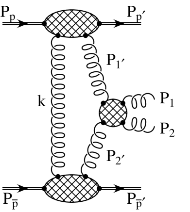
FIG. 4.: Our model of the Nonfactorizing (Lossless) Double Pomeron Exchange (N(L)DPE) amplitude with two gluon jets produced.

FIG. 5.: Double pomeron exchange (DPE) dijet production-CDF cuts. (a) Mean rapidity spectra $y_{+}\equiv(y_{1}+y_{2})/2$. (b) Ratio of mean rapidity spectra between the DPE and corresponding inclusive dijet processes. (c) $E_{T}$- Spectra. (d) Ratio of $E_{T}$-Spectra between the DPE and corresponding inclusive dijet processes.

FIG. 6.: Double pomeron exchange (DPE) dijet production - DØ1800 cuts. (a) Mean rapidity spectra $y_{+}\equiv(y_{1}+y_{2})/2$. (b) Ratio of mean rapidity spectra between the DPE and corresponding inclusive dijet processes. (c) $E_{T}$- Spectra. (d) Ratio of $E_{T}$-Spectra between the DPE and corresponding inclusive dijet processes.

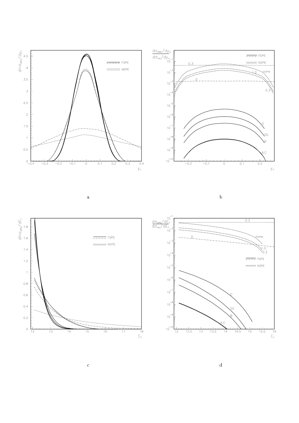
FIG. 7.: Double pomeron exchange (DPE) dijet production - DØ630 cuts. (a) Mean rapidity spectra $y_{+}\equiv(y_{1}+y_{2})/2$. (b) Ratio of mean rapidity spectra between the DPE and corresponding inclusive dijet processes. (c) $E_{T}$- Spectra. (d) Ratio of $E_{T}$-Spectra between the DPE and corresponding inclusive dijet processes.

FIG. 8.: Double pomeron exchange (DPE) dijet production - LHC cuts. (a) Mean rapidity spectra $y_{+}\equiv(y_{1}+y_{2})/2$. (b) Ratio of mean rapidity spectra between the DPE and corresponding inclusive dijet processes. (c) $E_{T}$- Spectra. (d) Ratio of $E_{T}$-Spectra between the DPE and corresponding inclusive dijet processes.

REFERENCES

- [1] V. N. Gribov, Zh. Eksp. Teor. Fiz. 41, 1962 (1961); V. N. Gribov and I. Ya. Pomeranchuk Phys. Lett. 9, 269, (1964).
- [2] T. Regge, Nuovo Cim. 14, 951 (1959).
- [3] G. Alberi and G. Goggi, Phys. Rept. 74, 1 (1981).
- [4] K. Goulianos, Phys. Rept. 101, 169 (1983).
- [5] J.C. Collins, D.E. Soper and G. Sterman, “Factorization of Hard Processes in QCD” in “Perturbative QCD” (A.H. Mueller, ed.) (World Scientific, Singapore, 1989).
- [6] J. C. Collins, D. E. Soper, and G. Sterman, Nucl. Phys. B261 (1985) 104; B308 (1988) 833; G. Bodwin, Phys. Rev. D 31 (1985) 2616; 34 (1986) 3932.
- [7] G. Ingelman and P.E. Schlein, Phys. Lett. B152, 256 (1985).
- [8] UA4 collaboration, M. Bozzo et al., Phys. Lett. B 155 (1985) 197; Phys. Lett. B 171 (1986) 142.
- [9] UA8 Collaboration, R. Bonino et al., Phys. Lett. B211, 239 (1988).
- [10] H. Fritzsch and K. K. Streng, Phys. Lett. B164, 391 (1985); K. H. Streng, Phys. Lett. B166, 443 (1986); K. H. Streng, Phys. Lett. B171, 313 (1986).
- [11] E.L. Berger, J.C. Collins, D.E. Soper and G. Sterman, Nucl. Phys. B286, 704 (1987).
- [12] A. Berera and D.E. Soper, Phys. Rev. D50, 4328 (1994).
- [13] A. Berera and D.E. Soper, Phys. Rev. D53, 6162 (1996).
- [14] L. Trentadue and G. Veneziano, Phys. Lett. B323, 201 (1994); M. Grazzini, L. Trentadue and G. Veneziano, Nucl. Phys. B519, 394 (1998).
- [15] J.C. Collins, Phys. Rev. D57, 3051 (1998).
- [16] J.C. Collins, L. Frankfurt and M. Strikman, Phys. Lett. B307, 161 (1993).
- [17] F. E. Low, Phys. Rev. D 12 (1975) 163; S. Nussinov, Phys. Rev. Lett. 34 (1975) 1286; Phys. Rev. D 14 (1976) 246.
- [18] J. F. Gunion and D. E. Soper, Phys. Rev. D15 (1977) 2617.
- [19] L. Frankfurt and M. Strikman, Phys. Rev. Lett. 63 (1989) 1914.
- [20] UA8 Collaboration, A. Brandt et al., Phys. Lett. B297, 417 (1992).
- [21] J. Pumplin, Phys. Rev. D52 (1995) 1477.
- [22] A. Berera and J.C. Collins, Nucl. Phys. B474, 183 (1996).
- [23] A. Bialas and P. V. Landshoff, Phys. Lett. B256 (1991) 540.
- [24] A. Bialas and W. Szeremeta, Phys. Lett. B296, 191 (1992).
- [25] F. Hautmann, Z. Kunszt, and D. E. Soper, Phys. Rev. Lett. 81, 3333 (1998); hep-ph/9906284.
- [26] A. Hebecker, Nucl. Phys. B585, 349 (1997).
- [27] K. Goulianos, Phys. Lett. B358, 379 (1995).
- [28] P.V. Landshoff and J. C. Polkinghorne, Nucl. Phys. B33, 221 (1971); B36, 642 (1972); F. Henyey and R. Savit, Phys. Lett. B52, 71 (1974); J. L. Cardy and G. A. Winbow, ibid B52, 95 (1974); C. DeTar, S. D. Ellis, and P. V. Landshoff, Nucl. Phys. B87, 176 (1975).
- [29] L. Alvero, J.C. Collins and J.J. Whitmore, hep-ph/9806340.
- [30] M. G. Albrow, CDF Collaboration, Fermilab-Conf-98/138-E “Di-jet Production by Double Pomeron Exchange in CDF”, contribution to LISHEP 98, Rio de Janeiro, February 1998.
- [31] K. Goulianos, CDF Collaboration, Proceedings of the XXXIInd Rencontre de Moriond, “QCD ’97 and High Energy Hadronic Interactions”, ed. J. Tran Thanh Van (Editions Frontieres), p. 447.
- [32] E. Gotsman, E. M. Levin, and U. Maor, Phys. Lett. B309, 199 (1993); 353, 526 (1995).
- [33] A. Rostovtsev and M. G. Ryskin, Phys. Lett. B390, 375 (1997).
- [34] E. Eichten, I Hinchliffe, K. Lane, and C. Quigg, Rev. Mod. Phys. 56, 579 (1984); 58, 1065 (1986).
- [35] A. Donnachie and P. V. Landshoff, Nucl. Phys. B191, 309 (1987); B303, 634 (1988).
- [36] L. Alvero, J.C. Collins, J. Terron and J.J. Whitmore, Phys. Rev. D59, 074022 (1999).
- [37] A. Donnachie and P. Landshoff, Nucl. Phys. B231 (1984) 189; Nucl. Phys. B244 (1984) 322.
- [38] A. Berera, “Factorization and Nonfactorization in Diffractive Hard Scattering”, contribution to DIS ‘97, Chicago, IL, April 1997, hep-ph/9707499.
- [39] A.D. Martin, M.G. Ryskin and V.A. Khoze, Phys. Rev. D56, 5867 (1997).
- [40] V.V. Sudakov, Sov. Phys. JETP 3, 65 (1956).
- [41] J.C. Collins, Phys. Rev. D22, 1478 (1980).
- [42] D. Joyce et al., Phys. Rev. D48, 1943 (1993).
- [43] P. Melese, CDF collaboration, “Diffractive Dijet Search with Roman Pots at CDF” Report No. Fermilab-Conf-96/231-E.
- [44] K. Terashi, CDF collaboration, “Observation of Dijet Production in Double Pomeron Exchange in Collisions at GeV”, contribution to Small x Meeting, Fermilab, IL, 1998.
- [45] R. Hirosky, DØ collaboration, “Jet Production with Two Rapidity Gaps”, contribution to LISHEP 98, Rio de Janeiro, February 1998.
- [46] K. Mauritz, DØ Collaboration, “Hard Diffraction at DØ ”, contribution to Small x Meeting, Argonne, IL, September 1996.
- [47] G. Alyes, DØ Collaboration, “Jet Production with Two Rapidity Gaps” contribution to Small x Meeting, Fermilab, IL, September 1998.
- [48] K. Mauritz, DØ Collaboration, “Hard Diffraction at DØ ”, contribution to DIS ‘99, Zeuthen, Germany, April 1999.
- [49] A. Brandt, DØ Collaboration, “DØ Run II Possibilities ”, presented at Physics at Run II Workshop, Fermilab, March 1999.
- [50] ZEUS Collaboration, M. Derrick et al., Z. Phys. C 68, 569 (1995); ZEUS Collaboration, M. Derrick et al., ibid 70, 391 (1996).
- [51] H1 Collaboration, C. Adloff et. al., Z. Phys. C 76, 613 (1997).
- [52] H. L. Lai et. al., CTEQ Collaboration, MSU-HEP-903100 hep-ph/9903282, 1999.
- [53] K. Terashi, private communication; M. G. Albrow, CDF Collaboration, talk presented at low x physics workshop, Tel Aviv, June 1999.
- [54] J.D. Bjorken, Phys. Rev. D47, 101 (1993).