FUTURE OF HEAVY-FLAVOUR PHYSICS

Abstract:

The prospects for the coming Golden Age of heavy-flavour physics are discussed from the perspective of one who hopes it may provide a window onto physics beyond the Standard Model. Precise QCD calculations are necessary for accurate determinations of CKM parameters, and may be provided by the lattice and new perturbative techniques. The future of CKMology in the wake of the relatively small branching ratio for $B_{d}\rightarrow\pi^{+}\pi^{-}$ are discussed, including alternative strategies for measuring $\alpha$ and $\gamma$. The opportunities for measurements of rare $B$ decays are reviewed briefly, as are possible $K$-decay windows on physics beyond the Standard Model, in the wake of the establishment of a relatively large value for $\epsilon^{\prime}/\epsilon$. Finally, relations to other aspects of flavour physics are discussed, including the grand unification of quark and lepton masses in the context of neutrino-mass models motivated by the recent oscillation data from Super-Kamiokande and elsewhere.
                                                    
                                     CERN-TH/99-318         hep-ph/9910404

1 Why Study Heavy Flavours ?

There are many honourable answers to this question: the subject has many challenging problems, perhaps it was your thesis topic, maybe you are in love with the Standard Model, or want to answer Rabi’s question about the muon: who ordered that? My personal perspective is based on the hope that heavy flavours may provide a welcome window on physics beyond the Standard Model. However, even if this window is closed, precision measurements of Standard Model parameters may provide welcome indirect clues, just as the measurement of $\sin^{2}\theta_{W}$ at LEP provided a hint of supersymmetric grand unification. But one should not exclude a priori the possibility that heavy flavours may finally extract us directly from our Standard Model straitjacket.

Heavy flavours are good places to look, because many new physics effects are suppressed by factors $\propto(E/M)^{n}$, where $E$ is the energy and $M$ is some large mass scale. Heavy flavours $Q$ provide ready-made high energies $E\sim m_{Q}$, so any new physics effects may be enhanced by comparison with light-flavour physics. The prime example is top physics [1]: in some models of flavour $m_{t}/M=0(1)$, and certainly the top quark Yukawa coupling $\lambda_{t}=0(1)$, so here may be the key that unlocks the door of flavour physics. As another example, we shall see later that in a class of supersymmetric GUT models $B(\tau\rightarrow\mu\gamma)\gg B(\mu\rightarrow e\gamma)$.

From this perspective, we need to understand QCD in order to do CKMology better, in the hope of finding some signature of physics beyond the Standard Model. This might either appear in the form of a (relatively) big contribution to a rare decay mode, e.g., perhaps $B(B_{d}\rightarrow\mu^{+}\mu^{-})>2\times 10^{-10}$ (the Standard Model prediction), or of a (relatively) small contribution to a common decay, e.g., perhaps the unitary triangle will turn out to be a quadrilateral?

In any case, the golden age of heavy flavours is surely now dawning. The era of precision electroweak physics is drawing to a close: the SLC has been terminated and LEP will cease operation in 2000. At the same time, new opportunities for precision flavour physics are opening up: BaBar, BELLE, CLEO III, CDF/D$\phi$ at RUN II, etc.

2 QCD Challenges

Even though $1\gg\alpha_{s}(m_{Q})$ in heavy-quark physics, the crucial challenge here is: how to calculate accurately in a theory whose perturbative expansion parameter $\alpha_{s}(m_{Q})\gg\alpha_{em}$ ? The traditional approximation scheme for any observable is to write it in the form

$$\sum_{n}~{}C_{n}(\alpha_{s}(\mu),{\Lambda\over\mu})<O_{n}(\mu)>$$ (1)

where the $C_{n}$ are coefficient functions, $\mu$ a factorization scale, and the $<O_{n}>$ operator matrix elements or condensates to be calculated non-perturbatively, e.g., using lattice techniques. Unfortunately, because of weakness and/or stupidity, we can only calculate to some finite order in $\alpha_{s}$. However, we know that the perturbation series is at best asymptotic, and there are in general renormalons. The scheme dependence they introduce can be absorbed into higher-twist terms, but we can only calculate a few of these, e.g., in heavy-quark effective theory (HQET) [2]. Not only are perturbative expansions asymptotic, but there may be effects that are invisible in any approximation scheme. As discussed here [3], there may be singularities away from the light-cone, at $|x^{2}|\not=0$, even $|x^{2}|\rightarrow\infty$. There are examples such as instantons and the ’t Hooft model of such breakdowns of duality, but the practical importance of such effects is not clear.

Some of the primary QCD puzzles in heavy-flavour physics are provided by production cross sections in hadron-hadron collisions. The Tevatron cross sections for $J/\psi$ and $\psi^{\prime}$ production [4] are much larger than expected in a naïve colour-singlet model, leading to the proposal of colour-octet dominance [5, 2]. This reproduces well the large-$p_{T}$ dependence, but the overall normalization is not well determined theoretically [6]. Since the colour-octet mechanism invokes soft E1 gluons that do not flip spin, it predicts large polarization [2]. However, this has not been seen [7, 4], either in charmonium or bottomonium production.

Naked heavy-flavour production is notoriously difficult to calculate [6]. Near threshold, there are large $[\alpha_{s}\ln^{2}(1-4m^{2}_{Q}/\hat{s})]^{n}$ corrections to be resummed, and at high energies there are large $[\alpha_{s}\ln(\hat{s}/4m^{2}_{Q}/)]^{n}$ effects. These provide potentially large enhancements, with $O(\Lambda/m_{Q})$ ambiguities at threshold. The cross section for $\bar{b}b$ production measured at the Tevatron collider [4] is about 2.5 times higher than the best theoretical prediction available. At HERA, the status of the theoretical predictions is particularly confusing [8]: $\sigma^{c}_{exp}/\sigma^{c}_{theory}\sim 1$, whilst $\sigma^{b}_{exp}/\sigma^{b}_{theory}\sim 4$! Of particular interest to HERA-B is the cross-section they should expect. Unfortunately, it is currently not possible for theory to provide precise guidance [6]: estimates lie in the range

$$\sigma^{b}_{\rm HERA-B}\sim 7.6~{}{\rm to}~{}45~{}{\rm mb}$$ (2)

with significant uncertainties associated with the choice of $m_{b},\mu$ and proton structure functions.

Heavy quarkonia offer interesting opportunities to determine $\alpha_{s}$, if the systematic errors in the required lattice calculations can be controlled to the level needed. The NRQCD value from the $\chi_{c}-J/\psi$ system is [2]

$$\alpha_{s}^{\overline{MS}}(M_{Z})=0.1174(15)~{}(19)~{}(\ldots)$$

whilst that obtained from the $\psi^{\prime}$ and $J/\psi$ is

$$\alpha_{s}^{\overline{MS}}(M_{Z})=0.1173(21)~{}(18)~{}(\ldots)$$

where in each case the last parenthesis $(\ldots)$ is to accommodate the lattice errors associated with the extrapolations needed in $m_{u,d,s}$ and sending the lattice size $a\rightarrow 0$. The values (2.3) are to be compared with

$$\alpha_{s}^{\overline{MS}}(M_{Z}) = 0.119\pm 0.002~{}~{}({\rm LEP}@Z~{}\cite[cite]{[\@@bibref{}{LEPEWWG}{}{}]})~{},$$ (4)

$$0.120\pm 0.003~{}(\tau~{}{\rm decay}~{}\cite[cite]{[\@@bibref{}{Davier}{}{}]})$$

The extension of NRQCD to the $\bar{t}t$ system can benefit from the extremely large mass of the $t$ quark and its relatively short lifetime, as in the potential NRQCD (PNRQCD) approach [11].

The numbers (2.3), (4) are of interest for testing supersymmetric GUT predictions. It is also possible to extract from $\tau$ decays [10, 12]

$$\overline{m_{s}}~{}(1~{}{\rm GeV})=234^{+61}_{-76}~{}{\rm MeV}$$ (5)

which is to be confronted with the lattice value [13]

$$\overline{m_{s}}~{}(1~{}{\rm GeV})=130~{}{\rm to}~{}180~{}{\rm MeV}$$ (6)

In addition to its great importance for QCD and CKMology, the value of $\overline{m_{s}}$ is also of interest for testing models of flavour. Bottomonium spectroscopy can be used to estimate $m^{\overline{MS}}_{b}(m_{b}^{\overline{MS}})$. Here, a significant advance has recently been made with the calculation of the two-loop lattice matching factor, which removes an ambiguity of several hundred MeV, resulting in the value [13]

$$m^{\overline{MS}}_{b}(m_{b}^{\overline{MS}})=4.3\pm 0.1~{}{\rm GeV}$$ (7)

A precise value for $m_{b}$ is also of interest for testing the predictions of GUTs [14] and models of flavour, as discussed later.

Other aspects of heavy-hadron spectroscopy discussed here, such as hybrids [15] and excited $D^{**}$ and $B^{**}$ states [16], have intrinsic QCD interest, but are not so important in a larger context.

Turning now to heavy-flavour decay matrix elements, it seems that lattice calculations are now taking over as the most precise for many applications. Compare, for example, the QCD sum-rule numbers for decay constants [17]:

$$f_{B} = 160\pm 30~{}{\rm MeV}~{},\quad f_{B_{s}/f_{B}}=1.16\pm 0.09$$

$$f_{D} = 190\pm 30~{}{\rm MeV}~{},\quad f_{D_{s}/f_{D}}=1.19\pm 0.08$$

which are ‘not improvable’ [17], with the unquenched lattice results [18]:

$$f_{B} = 210\pm 20~{}{\rm MeV}~{},\quad f_{B_{s}/f_{B}}=1.16\pm 0.04$$

$$f_{D} = 211\pm 30~{}{\rm MeV}~{},\quad f_{D_{s}/f_{D}}=1.11\pm 0.04$$

Also impressive are the recent lattice results for the $B$ parameters [18]:

$$B_{B}(m_{b})=0.80\pm 0.10~{},\quad B_{B_{s}}/B_{B_{d}}=1.00\pm 0.03$$ (10)

Also of direct experimental interest are the estimates [18]

$$\left({\Delta\Gamma\over\Gamma}\right)_{B_{S}}=0.16~{}(3)~{}(4)~{},\quad{\tau_{B^{-}}\over\tau_{B^{0}}}=1.03\pm 0.2\pm 0.3$$ (11)

The ratio $\tau_{\Lambda_{b}}/\tau_{B^{0}}$ could probably benefit from further analysis.

The lattice calculations of heavy-hadron semi-leptonic-decay form factors are now also very competitive [18, 19]. They can be calculated directly in the physical region of $q^{2}$, obviating the need for any extrapolation to extract CKM matrix elements.

The interpretation of non-leptonic $B$ decays has been beset by greater theoretical uncertainties, but there have recently been promising developments in the formulation of the problem [20]. A typical non-leptonic decay amplitude may be written schematically as

$$A={G_{F}\over\sqrt{2}}\sum_{n}V_{n}^{CKM}C_{n}(\mu)<F|Q_{n}(\mu)|B>$$ (12)

where our (my) primary objective is the extraction of the different CKM matrix elements $V_{n}^{CKM}$, and the essence of the problem is that the hadronic matrix elements $<F|Q_{n}(\mu)|B>$ are often not suitable for lattice evaluations. It is an old idea that these might factorize, e.g., in two-body decays:

$$<M_{1}M_{2}|Q|B>~{}\simeq~{}<M_{1}|J_{1}|B>~{}<M_{2}|J_{2}|0>$$ (13)

but several issues have been outstanding, e.g., the scheme and scale invariance, possible non-factorizable terms, final-state-interaction (FSI) phases, etc. A systematic extension to non-leptonic decays of the QCD factorization known in hadronic processes [21] has recently been made [20], as illustrated in Fig. 1, where there are two distinct contributions, distinguished by the hardness of the interactions with the spectator quark in the $B$ meson. In Fig. 1a, soft spectator interactions are subsumed in an exclusive form factor, there is a short-distance hadronic wave-function factor and a $2\rightarrow 2$ hard-scattering kernel $T_{I}$. In Fig. 1b, the spectator interactions are hard, and the factorization is into three short-distance wave functions and a $2\rightarrow 4$ hard-scattering kernel $T_{II}$. This approach formalizes perturbative QCD factorization and FSI, but does not include power corrections. Some of these could be important, particularly if they contain large chiral factors:

$$\left({\Lambda_{QCD}\over m_{b}}\right)\times{m^{2}_{\pi}\over\Lambda_{QCD}(m_{u}+m_{d})}\simeq{1\over 2}$$ (14)

is not very small!

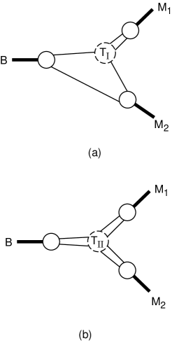
Figure 1: Contributions to the decay of a $B$ meson into two light mesons $M_{1,2}$, that may be factorized (a) with a $2\rightarrow 2$ hard-scattering kernel $T_{I}$, and (b) with a $2\rightarrow 4$ hard-scattering kernel $T_{ll}$ [20].

A useful phenomenological complement to this analysis is provided by diagramatic approaches based on Wick rotations [22, 23], as illustrated in Fig. 2, which can be improved using the renormalization group to become scale and scheme independent. In the honour of our Southampton hosts, I propose that Fig. 2a be baptized a ‘dolphin’ diagram . Note that Fig. 2b includes rescattering, as deconstructed in Fig. 2c.

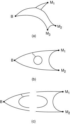
Figure 2: Examples of the renormalization-group-invariant classification of diagrams for $B$ decays [23], including (a) a ‘dolphin’ diagram for $B\rightarrow M_{1}+M_{2}+M_{3}$ decay, and (b) $B\rightarrow M_{1}+M_{2}$ decay, which may (c) be deconstructed to exhibit rescattering. The wavy lines denote generic-four-quark operators.

3 CKMology

Pride of place in this discussion goes to the unitarity triangle discussed here in more detail in [26], of which I now discuss various aspects in turn [27].

$\sin 2\beta$ : The theory of the CP-violating asymmetry in $B^{0}\rightarrow J/\psi~{}K_{S}$ decay is gold-plated, since the penguin contributions are expected to be very small, and FSI are unimportant [28]. This decay is also experimentally gold-plated, and the asymmetry has already been ‘measured’ by CDF [29]:

$$\sin 2\beta=0.79(39)~{}(16)$$ (15)

We will soon have $B$-factory measurements with a precision expected to attain $\pm$ 0.12 to 0.05 [30, 31], and eventually measurements at hadron machines may attain a precision $\pm$ 0.01. It should also be borne in mind that the available statistics could be doubled by including additional decay modes such as $B^{0}\rightarrow J/\psi K_{L}$, $\psi^{\prime}K_{S}$, etc. Measuring $\sin 2\beta$ does not determine $\beta$ uniquely, but the ambiguity could be removed by complementary measurements, e.g., comparing $B_{d}\rightarrow J/\psi K^{*}$ and $B_{s}\rightarrow J/\psi\phi$ can fix $\cos 2\beta$, and the cascade decay $B_{d}\rightarrow J/\psi(K^{0}\rightarrow\pi\ell\nu)$ can be used to measure $\cos 2\beta\sin(\Delta m_{K}t_{K})$ [28].

That was the good news $\ldots$ and now for the bad news $\ldots$

$\sin 2\alpha$ : The prime candidate for measuring this quantity was $B^{0}\rightarrow\pi^{+}\pi^{-}$, which was unseen by CLEO until just recently. The good news is that this mode has now been observed [32]:

$$B(B^{0}\rightarrow\pi^{+}\pi^{-})=(0.47^{+.18}_{-.15}\pm.13)\times 10^{-5}$$ (16)

but the bad news is that this is a factor $\sim 4$ below

$$B(B^{0}\rightarrow K^{+}\pi^{-})=(1.88^{+.28}_{-.26}\pm.06)\times 10^{-5}$$ (17)

The small ratio (16), (17) means that there must be considerable penguin pollution, which introduces ambiguity in the determination of $\sin 2\alpha$ [33], since penguins and trees have different phases. The improvement in theoretical calculations possible using isospin [34] or U-spin relations [35], or the new approach to amplitude factorization [20] may enable some of the penguin pollution to be cleaned up, but only a target error $\delta\alpha=\pm 10^{0}$ may be realistic. Under these circumstances, alternative ways to measure $\sin 2\alpha$ become more interesting. One suggestion [36] is the $B\rightarrow\rho\pi$ Dalitz plot, but here there are questions concerning the attainable statistics and the sensitivity in the presence of background, and another is to use $B\rightarrow D^{*\pm}\pi^{\mp}$ decays, which looks tough [28].

$\gamma$ : In view of the above imbroglio, in particular, there is increased interest in constraining and/or measuring $\gamma$. One line of attack [37] is to use $B^{\pm}\rightarrow\pi^{\pm}K^{0}$, $\pi^{0}K^{\pm}$ and $\pi^{\pm}\pi^{0}$ decays which receive contributions from penguins, electroweak penguins and tree diagrams (whose phase is $\gamma$). Using

$$R_{*}\equiv{B(B^{\pm}\rightarrow\pi^{\pm}K^{0})\over 2B(B^{\pm}\rightarrow\pi^{0}K^{\pm})}=0.47\pm 0.24$$ (18)

and $\bar{\epsilon}_{3/2}=0.24\pm 0.06,\delta_{EW}=0.64\pm 0.15$, in the inequality

$$R\equiv{1-\sqrt{R_{*}}\over\bar{\epsilon}_{3/2}}\leq|\delta_{EW}-\cos\gamma|+\ldots$$ (19)

where the dots denote small corrections, one finds the lower limit $\gamma>71^{0}$. It is possible, in principle, to extract $\gamma$ from the following combination of CP-violating asymmetries:

$$\tilde{A} \equiv {A_{CP}(\pi^{0}K^{\pm})\over R_{*}}-A_{CP}(\pi^{\pm}K^{0})$$ (20)

$$= 2\bar{\epsilon}_{3/2}\sin\gamma\sin\phi+\ldots$$

where $\phi$ is a strong-interaction phase: by measuring both $\tilde{A}$ and $R_{*}$, both $\gamma$ and $\phi$ can be determined [37].

Other channels offering prospects for measuring $\gamma$ include [28] $B^{\pm}\rightarrow{\buildrel(-)\over{D^{0}}}K^{\pm}$, ${\buildrel(-)\over{B^{0}}}\rightarrow D^{0}K^{*0}$, ${\buildrel(-)\over{B_{S}}}\rightarrow D^{\pm}_{s}K^{\mp}$ [38] and ${\buildrel(-)\over{B_{0}}}\rightarrow D^{*\pm}\pi^{\mp}$ [39], all of which may fairly be described as ‘challenging’. LHCb has studied, in particular, the second of these channels, and concludes that it could reach a precision of $\pm 10^{0}$ in $\gamma$. Hadron machines, such as the LHC, are clearly the ‘Promised Land’ for $B_{s}$ physics, which will surely flow with plenty of CP-violating ‘milk and honey’ [40].

4 Rare $B$ Decays

These offer good opportunities to measure Standard Model parameters [41], and may also be able to open windows on physics beyond the Standard Model [42].

As an example, $b\rightarrow s\gamma$ is related to $V_{st}$, and is also sensitive to $M_{H^{\pm}}$ and $(m_{\tilde{t}},m_{\chi^{\pm}})$ in supersymmetric extensions of the Standard Model. To make a precise calculation, one must resum the large QCD logarithms: $(\alpha_{s}/\pi)^{n+m}[\ln(m^{2}_{b}/M^{2})]^{m}$. In the Standard Model, the three-loop anomalous dimension and the two-loop matching conditions are known [43], so a relatively precise prediction can be made:

$$B(b\rightarrow s\gamma)=(3.32\pm 0.14\pm 0.26)\times 10^{-4}\phantom{\pm 0.2xx6}$$ (21)

This is to be compared with the experimental value:

$$B(b\rightarrow s\gamma)=(3.15\pm 0.35\pm 0.32\pm 0.26)\times 10^{-4}$$ (22)

There is some concern about the theoretical prediction of the $E_{\gamma}$ spectrum, and it might in principle be preferable to compare theory and experiment in a restricted and more reliable range [44], but there is certainly no hint yet of any need for physics beyond the Standard Model.

A NLO QCD calculation is available also in the MSSM [45], in the limit

$$\mu_{\tilde{g}} \equiv {\cal O}(m_{\tilde{g}},m_{\tilde{q}},m_{\tilde{t}_{1}})\gg\mu_{\tilde{w}}$$ (23)

$$\equiv {\cal O}(m_{W},m_{H^{\pm}},m_{\chi^{\pm}},m_{\tilde{t}_{2}})$$

The comparison between (21), (22) is an important constraint on the MSSM parameter space, as seen in Fig. 3 [46], where the NLO QCD calculation is used to exclude a region of parameter space that would otherwise be permitted for Higgsino cold dark matter. However, the available LO calculations are of limited accuracy when the simplified limit (23) is applicable, so it would be good to generalize the NLO QCD calculation beyond the region (23) of MSSM parameter space.

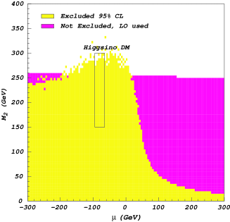
Figure 3: Regions of the $\mu,M_{2}$ plane of the MSSM which are allowed for Higgsino dark matter (rectangular box) but disallowed by the $b\rightarrow s\gamma$ analysis at NLO (light shaded region): the dark shading indicates a region allowed by a LO analysis. The following values of the other MSSM parameters have been chosen for this illustration: $m_{0}=1000$ GeV, $m_{A}=500$ GeV and tan$\beta=2.5$ [46].

The related decay $b\rightarrow d\gamma$ is equally calculable, and provides a way of measuring $V_{td}$. It may also provide an opportunity for physics beyond the Standard Model, such as supersymmetry.

The decays $b\rightarrow s,d\ell^{+}\ell^{-}$ provide additional opportunities for testing such theories, in particular via the measurement of a CP-violating forward-backward asymmetry. Personally, I also have a soft spot for $b\rightarrow s,d\bar{\nu}\nu$ decay, though this will be very difficult to observe.

The decay $B_{s}\rightarrow\mu^{+}\mu^{-}$ is expected to appear with a branching ratio of $(3.5\pm 0.1)\times 10^{-9}$ in the Standard Model. For comparison, the present experimental upper limit is $2.6\times 10^{-6}$. On the other hand, it should be measurable at the LHC: a CMS study indicates that as many as 26 events could be observed. Even the decay $B_{d}\rightarrow\mu^{+}\mu^{-}$ with an expected Standard Model branching ratio of $(1.5\pm 0.9)\times 10^{-10}$ may not lie beyond the reach of the LHC. CDF already has established an upper limit of $8.6\times 10^{-7}$, and CMS may be able to observe up to four events. These decays are vulnerable to physics beyond the Standard Model such as $R$ violation in supersymmetric models, and so could provide an interesting window on new physics.

5 Beyond the Standard Model ?

The best prospects for new physics at the TeV scale, and hence the most amenable to accelerator experiments, may be offered by the problem of mass, and hence associated with the Higgs sector and/or supersymmetry. In the MSSM, all the renormalizable couplings are related to those in the Standard Model, including the gauge coupling $g_{a}$, the Yukawa couplings $\lambda_{ijk}$ and their associated CKM phases. In addition, there are the standard soft supersymmetry-breaking parameters of the generic forms

$$(m^{2}_{0})^{j}_{i}\phi^{i}\phi^{*}_{j}~{},\quad{1\over 2}M_{a}\tilde{V}_{a}\tilde{V}_{a}~{},\quad A_{ijk}\lambda_{ijk}\phi^{i}\phi^{j}\phi^{l}$$ (24)

i.e., scalar and gaugino masses and soft trilinear couplings, respectively, and a term $B\mu\bar{H}H$ associated with Higgs mixing. There is no good theoretical reason known why the $(m^{2}_{0})^{j}_{i}$ should diagonalize in the same basis as the fermion masses, and they do not do so in generic string models, for example. However, there are important constraints on the $(m^{2}_{0})^{j}_{i}$ from flavour physics and CP physics [47], to which the most obvious solution is that they are universal [48]. There are in particular two CP-violating phases which are constrained by the experimental upper limits on the electric dipole moments of the electron and neutron, $d_{e}$ and $d_{n}$. The interpretation of $d_{e}$ is cleaner, since there are several different operators contributing to $d_{n}$ (e.g., involving $s$ quarks [49] as well as the valence $u$ and quarks), which could introduce cancellations, and hence make its interpretation more uncertain [50].

In addition to the above supersymmetric possibilities for new physics, one should also bear in mind the possibilities of non-standard soft super-symmetry-breaking terms [51]:

$$\phi^{i}\phi^{*}_{j}\phi^{*}_{k},\quad\phi^{i}\phi^{j}$$ (25)

where the $\phi^{i}$ are generic complex chiral scalar fields, and $R$-violating interactions [52].

The recent confirmation by KTeV [53] and NA48 [54] of the surprisingly large value of $\epsilon^{\prime}/\epsilon$ found previously by NA31 [55, 56] has rekindled interest in possible supersymmetric effects on CP-violating observables [57]. In the Standard Model, the first crude calculation was made in [58], and has subsequently been greatly refined - the fact that the data agree with the estimate $\epsilon^{\prime}/\epsilon\sim 1/450$ given in [58] is pure coincidence! One calculates nowadays [59, 60, 61, 62, 63]

$${\rm Re}\left({\epsilon^{\prime}\over\epsilon}\right)\simeq 13{\rm Im}\lambda_{t}\left({130~{}{\rm MeV}\over m_{s}(m_{c})}\right)^{2}\left({\Lambda^{(4)}_{\overline{MS}}\over 340~{}{\rm MeV}}\right)$$

$$\times\left[B_{6}(1-\Omega_{\eta\eta^{\prime}})-0.4B_{8}\left({m_{t}(m_{t})\over 165~{}{\rm GeV}}\right)^{2.5}\right]$$

(26)

where Im $\lambda_{t}=(1.33\pm 0.14)\times 10^{-4}$ is the CP-violating CKM factor, $B_{6}$ is a penguin operator matrix element factor estimated to be $1.0\pm 0.3$, $\Omega_{\eta\eta^{\prime}}$ is an electroweak penguin correction and $B_{8}$ is another matrix element factor estimated to be $0.8\pm 0.2$. Because of all the uncertainties [64] and the possibilities of cancellations, it is difficult to make a precise estimate of Re$(\epsilon^{\prime}/\epsilon)$. Formal analyses by two theoretical groups have recently yielded [59, 63]

$${\rm Re}\left({\epsilon^{\prime}\over\epsilon}\right)=(7.7^{+6.0}_{-3.5})\times 10^{-4}~{},\quad(4.7^{+6.7}_{-5.9})\times 10^{-4}$$ (27)

which might suggest a discrepancy with the experimental world average:

$${\rm Re}\left({\epsilon^{\prime}\over\epsilon}\right)=(21.2\pm 4.6)\times 10^{-4}$$ (28)

However, in view of the theoretical uncertainties, it seems safer to quote the following envelope of predictions [59]:

$$1\times 10^{-4}<{\rm Re}\left({\epsilon^{\prime}\over\epsilon}\right)<28\times 10^{-4}$$ (29)

which is not in significant disagreement with experiment (28). Nevertheless, it is clear that the measured value of Re$(\epsilon^{\prime}/\epsilon)$ tends to favour relatively large values of ${\rm Im}\lambda_{t},\Lambda^{(4)}_{\overline{MS}}$ and particularly $B_{6}$ [60, 63], as well as relatively small values of $B_{8},m_{s}$ and $m_{t}$. The least one can say, within the context of the Standard Model, is that the experimental value (28) requires big penguins: exotic [65] emperors, maybe?

This being said, even incorporating the constraints from $\epsilon^{\prime}/\epsilon$ and $K_{L}\rightarrow\mu^{+}\mu^{-}$, there is a window of opportunity for a significant contribution from CP violation beyond the Standard Model. One possibility is an enhanced $Zs\bar{d}$ vertex, which could enhance substantially the expected branching ratio for the rare CP-violating decay mode $K_{L}\rightarrow\pi^{0}\bar{\nu}\nu$, as well as $K_{L}\rightarrow\pi^{0}e^{+}e^{-}$ and $K^{+}\rightarrow\pi^{+}\bar{\nu}\nu$, so it would be interesting to push the experimental sensitivities for all these modes down to the Standard Model predictions, which are $B(K_{L}\rightarrow\pi^{0}\bar{\nu}\nu)=0.4\times 10^{-10}$, $B(K_{L}\rightarrow\pi^{0}e^{+}e^{-})=0.7\times 10^{-11}$ and $B(K^{+}\rightarrow\pi^{+}\bar{\nu}\nu)=1.1\times 10^{-10}$, respectively. They could be as large as $B(K_{L}\rightarrow\pi^{0}\bar{\nu}\nu)=1.2\times 10^{-10}$, $B(K_{L}\rightarrow\pi^{0}e^{+}e^{-})=2.0\times 10^{-11}$ and $B(K^{+}\rightarrow\pi^{+}\bar{\nu}\nu)=1.7\times 10^{-10}$, respectively [57].

There are many related opportunities for signatures of physics beyond the Standard Model in $b$ decays, notably [42]: squark mixing effects in $b\rightarrow d\gamma$? unexpected CP violation in $b\rightarrow s\gamma$? rate enhancements and CP-violating asymmetries in $b\rightarrow s,d\ell^{+}\ell^{-}$? enhanced rates for $B_{s,d}\rightarrow\mu^{+}\mu^{-}$? Other signatures to bear in mind are the possibilities that $B\rightarrow J/\psi K_{S}$, $\phi K_{S}$ and $D^{0}\pi^{0}$ might yield different values of $\beta$, and that the unitarity triangle could be distorted by new contributions to $B_{s}-\bar{B}_{s}$ mixing [66].

Although they lie beyond the limits of heavy-flavour physics, I should also like to advertize the physics interests of some related experiments. One is a proposal for a new-generation experiment on the neutron electric dipole moment. Another is the possibility that $\mu\rightarrow e\gamma$ decay might show up ‘close’ to the present experimental upper limit, which is motivated by the evidence for lepton flavour violation via neutrino oscillations, particularly in the context of supersymmetric GUTs [67]. A related heavy-flavour opportunity is provided by $\tau\rightarrow\mu/e\gamma$ decay: estimates in the same supersymmetric GUT framework suggest the possibility that $B(\tau\rightarrow e/\mu\gamma)\mathrel{\hbox to0.0pt{\raise 2.15277pt\hbox{$>$}\hss}{\lower 2.15277pt\hbox{$\sim$}}}10^{-9}$ [67], which might be accessible to CMS at the LHC.

6 Relations to Other Physics ?

We have already seen many potential interfaces of heavy-flavour physics with extensions of the Standard Model related to its outstanding problems of mass (via the Higgs sector and supersymmetry) and of unification (via GUTs). However, the outstanding contributions of the next generation of heavy-flavour experiments will surely be towards unravelling the problem of flavour, which is the most baffling puzzle raised by the Standard Model. It is not that we lack clues: the flavour sector contains at least 13 parameters (6 quark masses, 3 lepton masses and the 4 CKM angles), most of which have been measured to some level. Also, theorists abound with ideas, but their predictions are more often qualitative than quantitative. Perhaps the next generation of heavy-flavour experiments will provide more clues: it will certainly provide more precise measurements that may bust some of the GUT flavour models.

GUTs can predict quark masses in terms of lepton masses, because quarks and leptons are linked in common GUT multiplets. The prototype relation was [14]

$$m_{b}=m_{\tau}$$ (30)

before renormalization. The effective value of $m_{b}$ varies with the energy scale, as has been verified by DELPHI at LEP [68], and the renormalization group can be used to calculate the physical value of $m^{\overline{MS}}_{b}(m_{b}^{\overline{MS}})$ if one knows the spectrum of particles between here and $m_{GUT}$ (the Standard Model? the MSSM?). Starting from (30), such a calculation yields [69]

$$m^{\overline{MS}}_{b}(m_{b}^{\overline{MS}})\simeq 4.5~{}~{}{\rm to}~{}~{}5~{}~{}{\rm GeV}$$ (31)

in the MSSM, with the details depending on the sparticle thresholds, the appropriate value of $\alpha_{s}$, etc.

However, the analogous relations: $m_{s}\leftrightarrow m_{\mu}$ and $m_{d}\leftrightarrow m_{e}$ are unsuccessful, which is not surprising in the context of GUT models of flavour. These introduce higher-order terms in the mass matrices [70]:

$$m_{b}\left(\matrix{\epsilon^{n}&\epsilon^{m}&\epsilon^{p}\cr\epsilon^{m^{\prime}}&\epsilon^{q}&\epsilon^{r}\cr\epsilon^{p^{\prime}}&\epsilon^{r^{\prime}}&1}\right)\leftrightarrow m_{\tau}\left(\matrix{\epsilon^{\tilde{n}}&\epsilon^{\tilde{m}}&\epsilon^{\tilde{p}}\cr\epsilon^{\tilde{p}^{\prime}}&\epsilon^{\tilde{q}}&\epsilon^{\tilde{r}}\cr\epsilon^{\tilde{p}^{\prime}}&\epsilon^{\tilde{r}^{\prime}}&1}\right)$$ (32)

where $\epsilon$ is a small parameter, and the extra terms (which are indicated only in order of magnitude) may be related to non-renormalizable interactions and/or approximate symmetries: $U(1)$? a non-Abelian group?

New light on such models may be cast [71] by models of neutrino masses in GUTs and the emerging indications of neutrino oscillations. Most theoretical models of neutrino masses are based on the generic seesaw mechanism [72]:

$$(\nu_{L},\nu_{R})~{}~{}\left(\matrix{0&m\cr m^{T}&M}\right)~{}~{}\left(\matrix{\nu_{L}\cr\nu_{R}}\right)$$ (33)

where each entry is to be understood as a $3\times 3$ matrix in flavour space, the $\nu_{R}$ are right-handed singlet states, $m={\cal O}(m_{q},m_{\ell})$ and $M={\cal O}(m_{GUT})$ $\gg m_{W}$. After diagonalization, (33) yields light neutrino masses

$$m_{\nu}=m{1\over M}m^{T}$$ (34)

and one naturally obtains $m_{\nu}\sim 10^{-2}$ eV if, e.g., $m\sim$ 10 GeV and $M\sim 10^{13}$ GeV. Thanks to the matrices $m$ and $M$ appearing in (34), one can expect non-trivial mixing between the light-neutrino flavour eig- enstates, parametrized by a mixing matrix $V_{\nu}$, and there will in general also be mixing between the charged-lepton flavour eigenstates, parametrized by $V_{\ell}$. Thus we obtain a measurable neutrino mixing matrix [73] (between the neutrino and charged-lepton mass eigenstates) analogous to $V_{CKM}$:

$$V_{MNS}=V_{\ell}V^{\dagger}_{\nu}$$ (35)

The mixing observed experimentally might arise from $V_{\ell}$, or $V_{\nu}$, or both, and any mixing in $V_{\nu}$ might arise from $m$ or $M$, a priori. The neutrino mixing angles need not be small: one can easily construct models in which the powers of $\epsilon$ in the mass matrices (32) are different, the same is true a fortiori of $m$, and we have no hints about the structure of $M$ [74].

The indications from atmospheric neutrino data [75] are for maximal $\nu_{\mu}-\nu_{\tau}$ mixing with a difference in mass squared $\Delta m^{2}\sim 3\times 10^{-3}$ eV². The solar neutrino data indicate mixing of $\nu_{e}$ with $\nu_{\mu}$ and/or $\nu_{\tau}$, with three possible scenarios: $\Delta m^{2}\mathrel{\hbox to0.0pt{\raise 2.15277pt\hbox{$>$}\hss}{\lower 2.15277pt\hbox{$\sim$}}}10^{-5}$ eV² and large mixing, $\Delta m^{2}\sim 10^{-5}$ eV² and small mixing, or $\Delta m^{2}\sim 10^{-10}$ eV and large mixing. The last alternative may be disfavoured by the electron energy spectrum measured by Super-Kamiokande, and the second solar scenario is being constrained by constraints on a day-night difference in the Super-Kamiokande data. The first solar scenario will be probed by the KamLAND experiment, that is already observing reactor neutrinos. The atmospheric neutrino region will be probed by long-baseline accelerator neutrino experiments: K2K in Japan and MINOS in the U.S. are intended to look for $\nu_{\mu}$ disappearance, and the CERN-Gran Sasso project is intended primarily to search for $\nu_{\tau}$ appearance. The investment in these projects is modest compared to that in $B$ factories and experiments, but this may change. One of the interesting options for the future is a $\nu$ factory based on a muon storage ring [76], which may be able to extend the measurements of neutrino oscillations to CP-violating observables [77].

What does this (very) light-flavour physics have to do with heavy flavours? There are important implications for the interpretation of quark-lepton mass unification relations, and hence for theories of flavour [71]. One effect is a change in the mass renormalization at scales $\mu$: $m_{\nu_{R}}<\mu<m_{GUT}$, which we parametrize by $\xi_{N}$. A second effect is that non-trivial diagonalization of the lepton mass matrix (32) may alter significantly the relevant mass eigenvalue. For example, if

$$m^{0}_{D}=A\left(\matrix{C&0\cr 0&1}\right)~{},\quad m^{0}_{E}=\left(\matrix{x^{2}&x\cr x&1}\right)$$ (36)

one finds after diagonalization that

$${m_{D}\over m_{E}}={1\over 1+x^{2}}$$ (37)

As a result of these two effects, the appropriate extrapolated ratio to compare with GUT predictions is modified to [71]

$${\tilde{m}_{\tau}(m_{GUT})\over m_{b}(m_{GUT})}=(1+x^{2})~{}~{}\sqrt{{2\over 1+\xi^{2}_{N}}}$$ (38)

As a consequence, GUT mass unification can be maintained for any value of $\tan\beta$, the ratio of MSSM Higs vev’s, whereas it was often thought possible only for $\tan\beta$ either very large or very small.

7 May You Live in Interesting Times

This used to be considered a curse in ancient China, but may nowadays be considered a blessing. You are now entering what may turn out to be the Golden Age of heavy-flavour physics, with Babar, BELLE, CLEO III and HERA-B starting to take data, CDF and D$\phi$ soon returning to the fray, and LHCb and possibly BTeV on the horizon. In parallel with this experimental cornucopia, many theoretical tools are maturing, such as the lattice, HQET, (P)NRQCD, etc. Thus, you, the heavy-flavour community, will soon be having plenty of fun. You will be able to measure precisely the parameters of the Standard Model, perhaps revealing hints for new physics beyond the Standard model. If you are lucky, you may even find direct evidence for new physics. Happy hunting!

References

- [1] E. Simmons, hep-ph/9908488, and talk at this meeting.
- [2] I. Rothstein, talk at this meeting.
- [3] I. Bigi, M. Shifman, N. Uraltsev and A. Vainshtein, Phys. Rev. D59 (1999) 054011; M. Shifman, talk at this meeting
- [4] K. Sumorok, talk at this meeting.
- [5] E. Braaten and S. Fleming, Phys. Rev. Lett. 74 (1995) 3327.
- [6] P. Nason, talk at this meeting.
- [7] K. Seth, talk at this meeting.
- [8] C. Adloff et al., H1 Collaboration, hep-ex/9909029; F. Sefkow, talk at this meeting.
-
[9]
LEP Electroweak Working Group,
http://www.cern.ch/LEPEWWG. - [10] R. Barate et al., ALEPH Collaboration, hep-ex/9903015 and M. Davier, talk at this meeting.
- [11] M. Beneke, talk at this meeting.
- [12] See also A. Pich and J. Prades, JHEP 10 (1999) 004, who quote the value MeV.
- [13] G. Martinelli, talk at this meeting.
- [14] M.S. Chanowitz, J. Ellis and M.K. Gaillard, Nucl. Phys. B128 (1977) 506; A.J. Buras, J. Ellis, M.K. Gaillard and D.V. Nanopoulos, Nucl. Phys. B135 (1978) 66.
- [15] C. Michael, talk at this meeting.
- [16] V. Ciulli, talk at this meeting.
- [17] V. Braun, talk at this meeting.
- [18] S. Hashimoto, hep-latt/9909136 and talk at this meeting.
- [19] L. Lellouch, talk at this meeting.
- [20] M. Beneke, G. Buchalla, M. Neubert and C. Sachrajda, Phys. Rev. Lett. 83 (1999) 1914.
- [21] S.J. Brodsky and P. Lepage, Phys. Rev. D22 (1980) 2157.
- [22] M. Ciuchini, E. Franco, G. Martinelli and L. Silvestrini, Nucl. Phys. B501 (1997) 271.
- [23] A.J. Buras and L. Silvestrini, hep-ph/9812392; L. Silvestrini, talk at this meeting.
- [24] M. Shifman, hep-ph/9510397.
- [25] J. Ellis, M.K. Gaillard, D.V. Nanopoulos and S. Rudaz, Nucl. Phys. B131 (1977) 285.
- [26] S. Plaszczynski, talk at this meeting.
- [27] For a recent discussion by an expert, see: M. Gronau, hep-ph/9908343.
- [28] I. Dunietz, talk at this meeting.
- [29] T. Affolder et al., CDF Collaboration, hep-ex/9909003; D. Bortoletto, talk at this meeting.
- [30] R. Waldi, talk at this meeting.
- [31] S. Suzuki, talk at this meeting.
- [32] Y. Kwon et al., CLEO Collaboration, hep-ex/9908039; Y. Kubota, talk at this meeting.
- [33] See, for example, J. Charles, Phys. Rev. D59 (1999) 054007
- [34] M. Gronau and D. London, Phys. Rev. Lett. 65 (1990) 3381.
- [35] R. Fleischer, Phys. Lett. B459 (1999) 306.
- [36] H. Lipkin, Y. Nir, H. Quinn and A. Snyder, Phys. Rev. D44 (1991) 1454.
- [37] M. Gronau, J.L. Rosner and D. London, Phys. Rev. Lett. 73 (1994) 21; R. Fleischer, Phys. Lett. B365 (1996) 399; R. Fleischer and T. Mannel, Phys. Rev. D57 (1998) 2752; M. Gronau and J.L. Rosner, Phys. Rev. D59 (1999) 113002; A.J. Buras and R. Fleischer, hep-ph/9810260; M. Neubert and J.L. Rosner, Phys. Lett. B441 (1998) 403 and Phys. Rev. Lett. 81 (1998) 5076; M. Neubert, talk at this meeting.
- [38] R. Aleksan, I. Dunietz and B. Kayser, Z. Phys. C54 (1992) 653.
- [39] R. Fleischer, Int. J. Mod. Phys. A12 (1997) 2459; for further strategies using and/or decays, see: R. Fleischer, Eur. Phys. J. C10 (1999) 299.
- [40] N. Harnew, Nucl. Instrum. Meth. A408 (1998) 137, and talk at this meeting.
- [41] C. Greub, talk at this meeting.
- [42] A. Masiero, talk at this meeting.
- [43] M. Ciuchini, G. Degrassi, P. Gambino and G.F. Giudice, Nucl. Phys. B527 (1998) 21.
- [44] A.L. Kagan and M. Neubert, Eur. Phys. J. C7 (1999) 5.
- [45] M. Ciuchini, G. Degrassi, P. Gambino and G.F. Giudice, Nucl. Phys. B534 (1998) 3.
- [46] J. Ellis, T. Falk, G. Ganis, K.A. Olive, M. Schmitt and M. Spiropulu, in preparation.
- [47] J. Ellis and D.V. Nanopoulos, Phys. Lett. 110B (1982) 44.
- [48] R. Barbieri and R. Gatto, Phys. Lett. 110B (1982) 211.
- [49] J. Ellis and R. Flores, Phys. Lett. B377 (1996) 83.
- [50] A. Bartl, T. Gajdosik, W. Porod, P. Stockinger and H. Stremnitzer, Phys. Rev. D60 (1999) 073003.
- [51] I. Jack and D.R.T. Jones, Phys. Lett. B457 (1999) 101.
- [52] For a recent review, see: B.C. Allanach, A. Dedes and H.K. Dreiner, Phys. Rev. D60 (1999) 075014.
- [53] A. Alavi-Harati et al., KTeV Collaboration, Phys. Rev. Lett. 83 (1999) 22; A. Barker, talk at this meeting.
- [54] V. Fanti et al., NA48 Collaboration, hep-ex/9909022; P. Lubrano, talk at this meeting.
- [55] G.D. Barr et al., NA31 Collaboration, Phys. Lett. B317 (1993) 233.
- [56] For a recent discussion how to combine these results, see: G. D’Agostini, hep-ex/9910036.
- [57] A. Masiero and H. Murayama, Phys. Rev. Lett. 83 (1999) 907; R. Barbieri, R. Contino and A. Strumia, hep-ph/9908255; A.J. Buras, G. Colangelo, G. Isidori, A. Romanino and L. Silvestrini, hep-ph/9908371; G. Eyal, A. Masiero, Y. Nir and L. Silvestrini, hep-ph/9908382.
- [58] J. Ellis, M.K. Gaillard and D.V. Nanopoulos, Nucl. Phys. B109 (1976) 213.
- [59] S. Bosch, A.J. Buras, M. Gorbahn, S. Jager, M. Jamin, M.E. Lautenbacher and L. Silvestrini, hep-ph/9904408; A.J. Buras, hep-ph/9908395; M. Jamin, talk at this meeting.
- [60] S. Bertolini, J.O. Eeg, M. Fabbrichesi and E.I. Lashin, Nucl. Phys. B514 (1998) 93; S. Bertolini, M. Fabbrichesi and J.O. Eeg, hep-ph/9802405; M. Fabbrichesi, hep-ph/9909224.
- [61] T. Hambye, G.O. Kohler, E.A. Paschos and P.H. Soldanet, hep-ph/9906434.
- [62] A.A. Bel’kov, G. Bohm, A.V. Lanyov and A.A. Moshkin, hep-ph/9907335.
- [63] M. Ciuchini, E. Franco, L. Giusti, V. Lubicz and G. Martinelli, hep-ph/9910236 and hep-ph/9910237.
- [64] For a striking recent reminder of some of these uncertainties, see: T. Blum et al., hep-latt/9908025.
- [65] R. Fleischer and J. Matias, hep-ph/9906274.
- [66] A. Ali and D. London, hep-ph/9907243.
- [67] J. Ellis, M. Gomez, G. Leontaris, S. Lola and D.V. Nanopoulos, CERN preprint CERN-TH/99-237.
- [68] P. Abreu et al., DELPHI Collaboration, Phys. Lett. B418 (1998) 430.
- [69] M. Carena, M. Olechowski, S. Pokorski and C.E. Wagner, Nucl. Phys. B426 (1994) 269.
- [70] J. Ellis and M.K. Gaillard, Phys. Lett. 88B (1979) 315.
- [71] M. Carena, J. Ellis, S. Lola and C.E. Wagner, hep-ph/9906362.
- [72] M. Gell-Mann, P. Ramond and R. Slansky, Proceedings of the Stony Brook Supergravity Workshop, New York, 1979, eds. P. Van Nieuwenhuizen and D. Freedman (North-Holland, Amsterdam); T. Yanagida, Proceedings of the Workshop on Unified Theories and Baryon Number in the Universe, Tsukuba, Japan 1979, eds. A. Sawada and A. Sugamoto, KEK Report No. 79-18.
- [73] Z. Maki, M. Nakagawa and S. Sakata, Prog. Theor. Phys. 28, 247 (1962).
- [74] J. Ellis, G.K. Leontaris, S. Lola and D.V. Nanopoulos, Eur. Phys. J. C9 (1999) 389.
- [75] J.M. Conrad, Review Talk at 29th International Conference on High-Energy Physics (ICHEP 98), Vancouver, Canada, 23-29 Jul 1998, hep-ex/9811009.
- [76] Prospective study of muon storage rings at CERN, eds. B. Autin, A. Blondel and J. Ellis, CERN report 99-02.
- [77] S.M. Bilenkii, C. Giunti and W. Grimus, Phys. Rev. D58 (1998) 033001; A. De Rujula, M.B. Gavela and P. Hernandez, Nucl. Phys. B547 (1999) 21; V. Barger, Y. Dai, K. Whisnant and B. Young, Phys. Rev. D59 (1999) 113010; K.R. Schubert, hep-ph/9902215; M. Tanimoto, hep-ph/9906516; A. Donini, M.B. Gavela, P. Hernandez and S. Rigolin, hep-ph/9909254; A. Kalliomaki, J. Maalampi and M. Tanimoto, hep-ph/9909301; A. Romanino, hep-ph/9909425; M. Koike and J. Sato, hep-ph/9909469.