A New Approach to Weak Amplitudes in Large-$N_{C}$ QCD

Abstract

We report on some recent progress made in understanding weak matrix elements of mesons in the context of the next-to-leading order of the large-$N_{C}$ approximation to QCD. Specifically, we first use the example of the weak contributions to the $\pi^{+}-\pi^{0}$ mass difference to exhibit how a systematic matching can be achieved analytically between short distances and long distances within our large-$N_{C}$ framework. We are then also able to compute matrix elements of the operator $Q_{7}$, as they turn out to depend on the same QCD correlator as the previous pion mass difference. As a final example we determine the chiral counterterms governing the pseudoscalar decay into a lepton pair, where we briefly comment also on the special case $K_{L}\rightarrow\mu^{+}\mu^{-}$. This report covers the material presented by the authors in three separate talks at the QCD’99 conference in Montpellier.

1 INTRODUCTION

At the present level of accuracy, the simple description of electroweak interactions in the Standard Model gives an excellent fit to the experimental data at high energies collected over the last years, for instance at LEP [1]. For low-energy phenomenology however, the description in terms of the fields which appear in the Standard Model Lagrangian is inappropriate. It is more convenient to use an effective Lagrangian description where the heavy degrees of freedom of the Standard Model are integrated out in the presence of the strong interactions. This procedure leads, however, to a rather complicated structure for the weak processes involving hadrons. The effective Hamiltonian that describes the non-leptonic $\Delta S=1$ decay of kaons, for instance, is given by a set of four-quark operators $Q_{i}$,

$${\cal H}^{\mbox{\rm{\tiny eff}}}\,=\,\sum_{i}C_{i}(\mu)\ Q_{i}(\mu),$$ (1)

modulated by the functions $C_{i}(\mu)$, the Wilson coefficients, containing the information from the short-distance physics. The matching of the effective theory to the underlying theory of the Standard Model is performed at a high scale $\mu_{{\mbox{\tiny SM}}}\sim m_{\mbox{\tiny t}}\sim M_{W}$, where the corresponding Wilson coefficients $C_{i}(\mu_{{\mbox{\tiny SM}}})$ can be accurately computed in perturbation theory. In order to evaluate a weak matrix element at much lower energies $\mu\ll\mu_{{\mbox{\tiny SM}}}$, the Wilson coefficients are evolved downward using their renormalization group properties [2].

Physical observables evaluated with the effective Hamiltonian in Eq. (1) are independent of the arbitrary scale $\mu$ that was introduced in order to separate the short-distance physics, contained in the Wilson coefficients $C_{i}(\mu)$, from the long-distance contributions described by the hadronic matrix elements $<h^{\prime}|Q_{i}(\mu)|h>$ of the four-quark operators $Q_{i}(\mu)$. However, depending on the scale $\mu$ at which one is working, the contribution of a given operator $Q_{i}(\mu)$ can be more or less important, according to the behaviour of the modulating factor $C_{i}(\mu)$ under the renormalization group evolution. The latter is available only within a perturbative expansion in powers of the strong coupling constant $\alpha_{s}$. Although the present state of the art includes NNLO contributions[2] , it can only provide a reliable description of the scale dependence of the Wilson coefficients down to a scale $\mu$ which may, at best, be taken slightly below the charm quark mass, $\mu{\ \lower-1.2pt\vbox{\hbox{\hbox to0.0pt{$<$\hss}\lower 5.0pt\vbox{\hbox{$\sim$}}}}\ }m_{\mbox{\tiny c}}$. On the other hand, the computation of the matrix elements $<h^{\prime}|Q_{i}(\mu)|h>$ themselves requires non-perturbative methods. One possibility is to have recourse to numerical computations based on a discretized lattice version of QCD. Another approach consists in implementing in an analytic way some particular but systematic expansion scheme, like chiral perturbation theory (ChPT) and/or the large-$N_{C}$ expansion, etc. The fact that the final result for the matrix element $<h^{\prime}|{\cal H}^{\mbox{\rm{\tiny eff}}}|h>$ must then be independent of the factorization scale (at the given order of the non-perturbative expansion considered for the evaluation of the matrix elements of the four-quark operators) provides thus a non-trivial constraint and a crucial check of the whole calculation.

Finally, at a very low scale $\mu\ll 1$ GeV, the interactions of the light pseudoscalar mesons can be described within a systematic expansion in powers of momenta (chiral expansion). Indeed, in the chiral limit, these pseudoscalar states are the Goldstone bosons of spontaneous chiral symmetry breaking, so that their interaction becomes small at low energy. To lowest order in ChPT, their strong and weak matrix elements can be obtained, in the chiral limit, from the ${\cal O}(p^{2})$ chiral Lagrangian

$${\cal L}^{\mbox{\rm{\tiny eff}}}_{\chi}\,=\,{\cal L}^{(2)}_{S}+{\cal L}^{(2)}_{W;8}+{\cal L}^{(2)}_{W;27}\,,$$ (2)

where ${\cal L}^{(2)}_{S}$ accounts for the strong interactions between the pseudoscalars

$${\cal L}^{(2)}_{S}\,=\,-\frac{1}{F_{0}^{2}}\mbox{\rm tr}({\cal L}_{\mu}{\cal L}^{\mu}),$$ (3)

while the weak $|\Delta S|=1$ transitions receive contributions with the (8,1) quantum numbers of the chiral group $SU(3)_{L}\times SU(3)_{R}$

$${\cal L}^{(2)}_{W;8}\,=\,-4\frac{G_{F}}{\sqrt{2}}V_{ud}V_{us}^{*}g_{8}({\cal L}_{\mu})_{2i}({\cal L}_{\mu})_{i3}\,+\,{\mbox{h.c.}},$$ (4)

or with the (27,1) quantum numbers

$${\cal L}^{(2)}_{W;27} = -4\frac{G_{F}}{\sqrt{2}}V_{ud}V_{us}^{*}g_{27}\bigg{[}\frac{2}{3}({\cal L}_{\mu})_{21}({\cal L}_{\mu})_{13}$$ (5)

$$\qquad+({\cal L}_{\mu})_{23}({\cal L}_{\mu})_{11}\bigg{]}\,+\,{\mbox{h.c.}}\,.$$

Here we use the notation ${\cal L}_{\mu}=-i\frac{F_{0}^{2}}{2}U^{+}D_{\mu}U$, and as usual $U$ denotes a unitary $3\times 3$ matrix describing the octet of pseudoscalar fields. All strong and weak matrix elements involving only the Goldstone bosons can thus be evaluated at ${\cal O}(p^{2})$ accuracy and expressed in terms of only three low-energy constants, the decay constant of the pion in the chiral limit $F_{0}$, and the two constants $g_{8}$ and $g_{27}$ which, because of CP violation, are complex numbers. For instance, in this approximation, we obtain the following ratio of the $K\to(\pi\pi)_{I}$ amplitudes for the decay of kaons into two pions in a prescribed isospin channel $I=0,2$

$$\left|\frac{{\cal A}(K\to(\pi\pi)_{0})}{{\cal A}(K\to(\pi\pi)_{2})}\right|\,=\,\frac{1}{\sqrt{2}}\left|\frac{g_{8}+g_{27}}{g_{27}}\right|.$$ (6)

Higher order or quark mass corrections can, of course, be considered as well, but at the expense of introducing additional low-energy constants.

Unfortunately, an $a~{}priori$ knowledge of the values of the constants $g_{8}$ and $g_{27}$, which would lead to a quantitative understanding of the ratio in Eq.  (6), i.e. of the $\Delta I=1/2$ rule, is not available at present. Such a knowledge would require that one is actually able to continue the process of integrating out the high energy modes in (1) in a non-perturbative way down to the very low scale where the description in terms of the effective Lagrangian (2) is valid. On the other hand, these low-energy constants can be identified in terms of QCD correlators of bilinear quark operators. For instance, $F_{0}$ is exactly given by the following two-point correlator in the chiral limit and at zero momentum transfer:

$$\lim_{Q^{2}\to 0}\left(-Q^{2}\Pi_{LR}(Q^{2})\right)\,=\,F_{0}^{2},$$ (7)

where

$$\Pi_{LR}^{\mu\nu}(q) = 2i\!\int d^{4}x\,e^{iq\cdot x}\langle 0|\mbox{\rm T}\!\left(L^{\mu}(x)R^{\nu}(0)^{\dagger}\right)\!|0\rangle$$ (8)

$$= (\!q^{\mu}q^{\nu}\!-\!g^{\mu\nu}q^{2})\Pi_{LR}(Q^{2})\,,$$

with $Q^{2}=-q^{2}$, and where $L^{\mu}$ and $R^{\nu}$ are left- and right-handed currents with the appropriate flavour quantum numbers $e.g.$ $L_{\mu}\,=\,{\overline{u_{L}}}\gamma_{\mu}d_{L}$, $R_{\mu}\,=\,{\overline{u_{R}}}\gamma_{\mu}d_{R}$. The low-energy constants of the strong interaction part ${\cal L}^{\mbox{\rm{\tiny eff}}}_{S}=\sum_{n\geq 1}{\cal L}^{(2n)}_{S}$ describing higher orders in the chiral expansion can likewise be expressed in terms of the low-momentum behaviour of QCD correlators. For instance, one of the Gasser-Leutwyler constants [3] at order ${\cal O}(p^{4})$, $L_{10}$, is given by the coefficient of the secont term in the expansion of $-Q^{2}\Pi_{LR}(Q^{2})$, i.e.

$$-Q^{2}\Pi_{LR}(Q^{2})\,=\,F_{0}^{2}+4L_{10}Q^{2}+{\cal O}(Q^{4})\,,$$ (9)

modulo chiral logarithms that we have not displayed explicitly. In general, one can find an analogous representation for the other low-energy constants of ${\cal L}^{\mbox{\rm{\tiny eff}}}_{S}$ as coefficients of a Taylor expansion around zero momentum of certain Green functions, but not always two-point Green functions. Using dispersion relations, one may then express these low-energy constants in terms of observables of the hadronic spectrum in the chiral limit. As a matter of fact, the low-energy constants of interest, such as $F_{0}$, and the corresponding Green’s functions, such as $\Pi_{LR}^{\mu\nu}(q)$, happen to be order parameters of chiral symmetry breaking. This means that these Green’s functions, which receive no contribution from the pertubative QCD continuum, behave smoothly at short distances, and that the corresponding dispersion relations converge therefore rapidly. In practice, one may thus expect to need information on the hadronic spectrum only over a finite energy range, say up to $\sim$1 GeV. Unfortunately such data, even away from the chiral limit, are not always available. An enormous simplification comes about after taking the large-$N_{C}$ limit of QCD. In this limit the spectrum consists of an infinite number of zero-width mesonic resonances. For instance, $\Pi_{LR}(Q^{2})$ is then given by the pion pole and by an infinite sum over single particle vector and axial-vector states, i.e.

$$-Q^{2}\Pi_{LR}(Q^{2})=F_{0}^{2}\qquad\qquad\qquad\qquad$$

$$+Q^{2}\sum_{A}\frac{f_{A}^{2}M_{A}^{2}}{M_{A}^{2}+Q^{2}}-Q^{2}\sum_{V}\frac{f_{V}^{2}M_{V}^{2}}{M_{V}^{2}+Q^{2}}\,,$$ (10)

which, upon expanding the above large-$N_{C}$ representation of $-Q^{2}\Pi_{LR}(Q^{2})$ around $Q^{2}=0$, yields the following expression for $L_{10}$ [4][5],

$$4L_{10}=\sum_{A}f_{A}^{2}-\sum_{V}f_{V}^{2}\,,$$ (11)

in terms of the parameters of the zero-width mesonic resonances.

The situation is more involved when it comes to the constants occurring in the $|\Delta S|=1$ sector, such as $g_{8}$ or $g_{27}$. Although they can still be expressed in terms of QCD four-point functions of quark bilinears which are order parameters of spontaneous chiral symmetry breaking, they involve for instance two left-handed charged currents convoluted with a free $W$-boson propagator. Therefore, the whole range of momenta, and not only the low-momentum region, is involved. The same happens to the constants describing electromagnetic corrections to strong processes.

The crucial question is of course whether this interpolation at large $N_{C}$ can be realized in a way that provides the correct matching of the scale dependence of the weak matric elements $<h^{\prime}|Q_{i}(\mu)|h>$ with the scale dependence of the short-distance piece encoded in the Wilson coefficients, $C_{i}(\mu)$. As we shall see, there are some observables where we have already been able to realize this program.

2 A CLASSIC EXAMPLE REVISITED

In the chiral limit the $\pi$, the $K$ and the $\eta$ form an octet of massless Goldstone bosons, provided electroweak interactions are neglected. In the presence of electromagnetic interactions, however, the electrically charged members of the erstwhile octet of Goldstone bosons acquire a mass even in the chiral limit. This mass term can be described by the effective operator

$${\cal L}^{\mbox{\rm{\tiny eff}}}_{mass;\gamma}\,=\,4\pi\alpha C_{\gamma}\,\mbox{\rm tr}\left(Q_{R}UQ_{L}U^{\dagger}\right)\qquad\qquad$$

$$\qquad\,=\,-8\pi\alpha C_{\gamma}\frac{1}{F_{0}^{2}}(\pi^{+}\pi^{-}+K^{+}K^{-})+\cdots\,,$$ (12)

where $Q_{R,L}$ are matrices of charges in flavour space governing the couplings of quarks to the photon, $Q_{R}\!=\!Q_{L}\!=\!\mbox{\rm diag}[2/3,-1/3,-1/3]$, and $\alpha$ is the fine structure constant. The constant $C_{\gamma}$ results from integrating out all degrees of freedom but the Goldstone bosons and the photon in the Standard Model Lagrangian. The fact that the QCD part is described in terms of quarks and gluons and not in terms of hadrons is of course a good part of the difficulty in performing this integration.

In this classic example, it is well known that $C_{\gamma}$ is determined by the same two-point function $\Pi_{LR}(Q^{2})$ that we have already encountered [6], but contrary to $F_{0}$ or to $L_{10}$, which describe its low-momentum behaviour, the identification of $C_{\gamma}$ involves an integral of $\Pi_{LR}(Q^{2})$, weighted with the free photon propagator, over the whole range of momenta,

$$C_{\gamma}=-\frac{1}{8\pi^{2}}\,\frac{3}{4}\int_{0}^{\infty}dQ^{2}\,Q^{2}\Pi_{LR}(Q^{2}).$$ (13)

We stress here that $C_{\gamma}$ is thus very akin to the coupling constants in the chiral Lagrangian describing electroweak interactions of hadrons, such as $g_{8}$ or $g_{27}$ for instance.

The integral in (13) can be split-off at an arbitrary intermediate scale $\Lambda$, but large enough that perturbation theory sets in [7]. The high-momentum region of integration, $Q^{2}\gg\Lambda^{2}$, can be evaluated upon taking for $\Pi_{LR}(Q^{2})$ its asymptotic behaviour at short distances, which in QCD is given by (this property ensures the convergence of Eq. (13))

$$\lim_{Q^{2}\rightarrow\infty}Q^{4}\Pi_{LR}(Q^{2})\,=\,0\,,$$ (14)

and

$$\lim_{Q^{2}\rightarrow\infty}Q^{6}\Pi_{LR}(Q^{2})=\qquad\qquad\qquad\qquad$$

$$-4\pi^{2}\left(\frac{\alpha_{s}}{\pi}+{\cal O}(\alpha_{s}^{2})\right)\langle\bar{\psi}\psi\rangle^{2}\,.$$ (15)

Notice that in the last formula, we have already replaced the relevant four-quark condensate by its factorized large-$N_{C}$ expression. For the large-$N_{C}$ limit representation in Eq. (1), these properties translate into the first and second Weinberg sum rules [8]

$$\sum_{V}f_{V}^{2}M_{V}^{2}-\sum_{A}f_{A}^{2}M_{A}^{2}=F_{0}^{2},$$ (16)

$$\sum_{V}f_{V}^{2}M_{V}^{4}-\sum_{A}f_{A}^{2}M_{A}^{4}=0,$$ (17)

and into the relation [5]

$$\sum_{V}f_{V}^{2}M_{V}^{6}-\sum_{A}f_{A}^{2}M_{A}^{6}=\qquad\qquad\qquad\qquad$$

$$-4\pi^{2}\left(\frac{\alpha_{s}}{\pi}+{\cal O}(\alpha_{s}^{2})\right)\langle\bar{\psi}\psi\rangle^{2}\ ,\$$ (18)

respectively. The corresponding contribution to $C_{\gamma}$ from the high-momentum part of the integral reads

$$C_{\gamma}^{>}(\Lambda)\,=\,+\frac{3}{8}\left(\frac{\alpha_{s}}{\pi}+{\cal O}(\alpha_{s}^{2})\right)\frac{\langle\bar{\psi}\psi\rangle^{2}}{\Lambda^{2}}$$

$$\qquad\qquad+{\cal O}\left(\frac{1}{\Lambda^{4}}\right)\,.$$ (19)

For the low-momentum region of the integral, the large-$N_{C}$ representation of Eq. (1) gives

$$C_{\gamma}^{<}(\Lambda)\,=\qquad\qquad\qquad\qquad\qquad\qquad\qquad\qquad$$

$$+\frac{3}{32\pi^{2}}\bigg{[}\sum_{A}f_{A}^{2}M_{A}^{4}\ln\frac{M_{A}^{2}}{\Lambda^{2}}-\sum_{V}f_{V}^{2}M_{V}^{4}\ln\frac{M_{V}^{2}}{\Lambda^{2}}\bigg{]}$$

$$+\frac{3}{32\pi^{2}}\ \ \frac{\sum_{V}f_{V}^{2}M_{V}^{6}-\sum_{A}f_{A}^{2}M_{A}^{6}}{\Lambda^{2}}\qquad\qquad\qquad$$

$$+{\cal O}\left(\frac{1}{\Lambda^{4}}\right)\ ,\qquad$$ (20)

after using the two Weinberg sum rules (16) and (17). Upon adding the two pieces, one obtains a perfect matching to the given order in $1/\Lambda$, i.e. $C_{\gamma}^{<}(\Lambda)+C_{\gamma}^{>}(\Lambda)\sim{\cal O}(1/\Lambda^{4})$, due to the sum-rule in Eq. (2). Clearly this cancellation can be effected to any order in $1/\Lambda$, as Eq. (13) has no $\Lambda$ to begin with, but the point is that, in order to accomplish this $\Lambda$ matching, care must be taken that the constraints imposed by the OPE are satisfied to that order in $1/\Lambda$ [5]. This lesson is very important in the case of weak matrix elements.

Let us notice here that a simple ansatz that realizes all the properties listed above consists in taking into account only one vector and one axial-vector resonance (satisfying even some other stronger constraints discussed in Ref.[9]) that we shall call the Lowest Meson Dominance (LMD) approximation to large-$N_{C}$ QCD. In this case one has the simpler expression [7]

$$-Q^{2}\Pi_{LR}^{\mbox{\tiny{LMD}}}(Q^{2})\,=\,\frac{M_{\rho}^{2}M_{a1}^{2}F_{0}^{2}}{(Q^{2}+M_{\rho}^{2})(Q^{2}+M_{a1}^{2})}\,,$$ (21)

where $M_{\rho}^{2}=\frac{3\sqrt{6}}{5N_{C}}(4\pi F_{0})^{2}$, $M_{a1}=\sqrt{2}M_{\rho}$ [9] and $F_{0}\simeq 87$MeV is an estimate of the pion decay constant in the chiral limit [4][3]. Combining Eqs. (2,13) and (21) one obtains

$$m_{\pi^{+}}^{2}=F_{0}^{2}\ \frac{24\sqrt{6}}{5}\pi\alpha\ln 2\quad,$$ (22)

i.e. $m_{\pi^{+}}-m_{\pi^{0}}\simeq\ 5$ MeV to be compared to $m_{\pi^{+}}-m_{\pi^{0}}|_{exp}\simeq 4.6$ MeV.

In order to create a situation which is more similar to the one encountered in the case of the $|\Delta S|=1$ transitions, let us rather consider the masses acquired by the pseudoscalar octet under the influence of the weak neutral currents [10]. They result from an effective term similar to (2)

$${\cal L}^{\mbox{\rm{\tiny eff}}}_{mass;Z^{0}}=4\pi\alpha C_{Z}\,\mbox{\rm tr}\left(Q_{R}UQ_{L}U^{\dagger}\right)\,,$$ (23)

but with a coupling constant $C_{Z}$ which involves the integral of $\Pi_{LR}(Q^{2})$ weighted by the propagator of the massive $Z^{0}$,

$$C_{Z}=\frac{1}{8\pi^{2}}\,\frac{3}{4}\int_{0}^{\infty}dQ^{2}\,\frac{Q^{2}}{Q^{2}+M_{Z}^{2}}\,Q^{2}\Pi_{LR}(Q^{2}).$$

The change of sign as compared to Eq. (13) is a consequence of the $SU(2)\times U(1)$ quantum numbers of the quarks. Using an Euclidean momentum cutoff $\Lambda$, one may again split the integral into a low-energy piece, which gives

$$C_{Z}^{<}(\Lambda)\,=\,\frac{3}{32\pi^{2}}\frac{1}{M_{Z}^{2}}\bigg{[}\sum_{A}f_{A}^{2}M_{A}^{6}\ln\frac{M_{A}^{2}}{\Lambda^{2}}$$

$$-\sum_{V}f_{V}^{2}M_{V}^{6}\ln\frac{M_{V}^{2}}{\Lambda^{2}}\bigg{]}\,,$$ (25)

and a high-energy piece, evaluated with the leading short-distance behaviour given by Eq. (2),

$$C_{Z}^{>}(\Lambda)\,=\,-\frac{3}{8\pi}\frac{1}{M_{Z}^{2}}\alpha_{s}\langle\bar{\psi}\psi\rangle^{2}\,\,\ln\frac{M_{Z}^{2}}{\Lambda^{2}}.$$ (26)

Adding Eqs. (2) and (26) one obtains the final result which is, of course, $\Lambda$ independent.

A more common approach is to construct an effective Lagrangian in which the $Z^{0}$ has been integrated out and the Green functions are renormalized using the $\overline{MS}$ scheme. The relevant term in the Lagrangian of the Standard Model which is responsible for the $Z$-induced contribution to the $\pi^{+}-\pi^{0}$ mass difference is the neutral current interaction term

$${\cal L}_{\mbox{\rm{\tiny NC}}}=\frac{e}{2\sin\theta_{W}\cos\theta_{W}}\bigg{[}\bar{q}_{L}\gamma^{\mu}T_{3}q_{L}$$

$$\qquad-2\sin^{2}\theta_{W}\bar{q}_{L}\gamma^{\mu}Q_{L}q_{L}$$

$$\qquad-2\sin^{2}\theta_{W}\bar{q}_{R}\gamma^{\mu}Q_{R}q_{R}\bigg{]}Z_{\mu}\,.$$ (27)

When looking for the induced effective Lagrangian of order ${\cal O}(p^{0})$ which contributes to Goldstone boson masses, it is sufficient to consider left-right operators. In the absence of the strong interactions, the effective four-quark Hamiltonian which emerges after integrating out the $Z$ field is

$$-{\cal H}_{\mbox{\rm{\tiny NC}}}^{\mbox{\rm{\tiny eff}}}=\frac{-1}{M_{Z}^{2}}\frac{e^{2}}{\cos^{2}\theta_{W}}\times\qquad\qquad\qquad$$

$$\bigg{[}\sin^{2}\theta_{W}Q_{LR}-\frac{1}{2}\left(\bar{q}_{L}\gamma_{\mu}T_{3}q_{L}\right)\left(\bar{q}_{R}\gamma^{\mu}Q_{R}q_{R}\right)\bigg{]}$$

$$=\frac{e^{2}}{M_{Z}^{2}}Q_{LR}\qquad\qquad\qquad\qquad\qquad\qquad\qquad$$

$$-\frac{e^{2}}{M_{Z}^{2}}\frac{1}{\cos^{2}\theta_{W}}\frac{1}{6}\left(\sum_{q}\bar{q}\gamma_{\mu}q\right)\left(\bar{q}_{R}\gamma^{\mu}Q_{R}q_{R}\right)\ ,$$

where

$$Q_{LR}\equiv\left(\bar{q}_{L}\gamma_{\mu}Q_{L}q_{L}\right)\left(\bar{q}_{R}\gamma^{\mu}Q_{R}q_{R}\right)\,,$$ (29)

and summation over quark colour indices within brackets is understood. In fact, to ${\cal O}(p^{0})$, only the first term proportional to the four-quark operator $Q_{LR}$ can contribute. In the presence of the strong interactions, the evolution of $Q_{LR}$ from the scale $M_{Z}^{2}$ down to a scale $\mu^{2}$ can be calculated in the usual way, provided this $\mu^{2}$ is still large enough for a perturbative QCD (pQCD) evaluation to be valid. In the leading logarithmic approximation in pQCD, and to leading non–trivial order in the $1/N_{C}$ expansion, the relevant mixing in this evolution which we need to retain is simply given by

$$Q_{LR}(M_{Z}^{2})=Q_{LR}(\mu^{2})\qquad\qquad\qquad\qquad$$

$$-3\frac{\alpha_{\mbox{\rm{\scriptsize s}}}}{\pi}\frac{1}{2}\log\frac{M_{Z}^{2}}{\mu^{2}}D_{RL}(\mu^{2})$$

$$+\cdots$$ (30)

where $\mu$ is the $\overline{MS}$ scale and $D_{RL}$ denotes the four-quark density-density operator

$$D_{RL}\equiv\sum_{q,q^{\prime}}e_{q}e_{q^{\prime}}(\bar{q^{\prime}}_{L}q_{R})(\bar{q}_{R}q^{\prime}_{L})\,,$$ (31)

with $e_{q}$ and $e_{q^{\prime}}$ the quark charges in units of the electric charge. This can be seen as follows: in the $\overline{MS}$ renormalization scheme, the full evolution of the Wilson coefficients $c_{Q}$ and $c_{D}$ of the operators $Q_{LR}$ and $D_{LR}$ at the one-loop level is governed by the equations (subleading contributions in the $1/N_{C}$ expansion have been neglected)

$$\mu^{2}\frac{d}{d\mu^{2}}\left(\begin{array}[]{c}c_{Q}\\ c_{D}\end{array}\right)=\qquad\qquad\qquad\qquad\qquad$$ (34)

$$\frac{1}{4}\frac{\alpha_{\mbox{\rm{\scriptsize s}}}N_{C}}{\pi}\left(\begin{array}[]{cc}\cdots&\cdots\\ \frac{6}{N_{C}}&-3+\cdots\end{array}\right)\left(\begin{array}[]{c}c_{Q}\\ c_{D}\end{array}\right)\,,$$ (39)

with boundary conditions: $c_{Q}(M_{Z})=1$ and $c_{D}(M_{Z})=\frac{3}{2}\frac{\alpha_{\mbox{\rm{\scriptsize s}}}}{\pi}$. The result in eq. (2) follows when taking $c_{D}(M_{Z})=0$, which is appropriate when keeping the one–loop leading log only, and from the off–diagonal term in the (transposed) anomalous dimension matrix.

We are then confronted with a typical problem of bosonization of four-quark operators. The bosonization of $D_{RL}$ is only needed to leading order in the $1/N_{C}$ expansion. To that order and to order ${\cal O}(p^{0})$ in the chiral expansion it can be readily obtained from the bosonization of the factorized density currents, with the result 

$$D_{RL}\equiv\sum_{q,q^{\prime}}e_{q}e_{q^{\prime}}(\bar{q^{\prime}}_{L}q_{R})(\bar{q}_{R}q^{\prime}_{L})\qquad\rightarrow$$

$$\left(\frac{\langle{\bar{\psi}}\psi\rangle}{2}\right)^{2}\,\mbox{\rm tr}\left(UQ_{L}U^{\dagger}Q_{R}\right)\,.$$ (40)

We find that the overall contribution of the term proportional to the $D_{RL}(\mu^{2})$ four–quark operator, which we denote $C_{Z}|_{D_{RL}}$, is given by the expression

$$C_{Z}|_{D_{RL}}=\frac{-3}{8\pi}\frac{1}{M_{Z}^{2}}\alpha_{\mbox{\rm{\scriptsize s}}}\langle\bar{\psi}\psi\rangle^{2}\log\frac{M_{Z}^{2}}{\mu^{2}}\,,$$ (41)

and it is exactly the same result as the one coming from the $d=6$ term of the OPE in the previous calculation of Eq. (26), except for the difference between $\mu$ and $\Lambda$.

The problem is then reduced to the bosonization of the operator $Q_{LR}(\mu^{2})$. We are confronted here with a typical calculation of a hadronic matrix element of a four-quark operator, in this case the matrix element $\langle\pi^{+}|Q_{LR}(\mu^{2})|\pi^{+}\rangle$. The factorized component of the operator $Q_{LR}$, which is leading in $1/N_{C}$, cannot contribute to the ${\cal O}(p^{0})$ term of the low-energy effective Lagrangian. The contribution we want from this matrix element is therefore the next-to-leading one in the $1/N_{C}$ expansion.

The calculation proceeds along much the same lines as first suggested in papers by Bardeen, Buras and G érard [12] sometime ago , except that we shall go beyond loops generated by Goldstone particle interactions alone in order to achieve a correct matching with the logarithmic scale dependence of the short–distance contribution in eq. (41). We can evaluate now the matrix element $\langle\pi^{+}|Q_{LR}(\mu^{2})|\pi^{+}\rangle$ within the framework of an effective Lagrangian which is a straightforward generalization to an arbitrary number of massive $J^{P}=1^{-}$ and $J^{P}=1^{+}$ mesonic states of the effective Lagrangian corresponding to the LMD approximation to QCD$(\infty)\;$recently discussed in ref. [9]. Furthermore we shall do so by using an Euclidean momentum cutoff to study the issue of regularization. We leave the details of the calculation to our work in Ref. [10]. The final result reads

$$C_{Z}|_{Q_{LR}}=-\frac{F_{0}^{2}}{2M_{Z}^{2}}\langle\pi^{+}|Q_{LR}(\mu^{2})|\pi^{+}\rangle\quad{\mbox{\rm with}}$$

$$\langle\pi^{+}|Q_{LR}(\mu^{2})|\pi^{+}\rangle=\qquad\qquad\qquad\qquad\qquad$$

$$\frac{+1}{16\pi^{2}}\bigg{\{}\frac{3}{2}\mu^{4}+4\frac{L_{10}}{F_{0}^{2}}\mu^{6}\qquad\qquad\qquad\qquad\qquad$$

$$+\frac{3}{F_{0}^{2}}\int_{0}^{\mu^{2}}dQ^{2}Q^{6}\qquad\qquad\qquad\qquad\qquad$$

$$\quad\qquad\times\bigg{[}\sum_{V}\frac{f_{V}^{2}}{Q^{2}+M_{V}^{2}}-\sum_{A}\frac{f_{A}^{2}}{Q^{2}+M_{A}^{2}}\bigg{]}\bigg{\}}\,.$$ (42)

The contribution of the Goldstone bosons alone corresponds to the two terms in the first line of the r.h.s. of Eq. (2). They display a typical polynomial dependence with respect to the cut-off $\mu$, which can hardly provide a reasonably good matching with the logarithmic scale dependence coming from the short–distance contributions in $C_{Z}|_{D_{RL}}$. In fact, in an $\overline{MS}$ regularization scheme, as commonly chosen for the evaluation of the short-distance Wilson coefficients, these power divergences will automatically disappear. Simply adding higher resonances does not by itself solve the problem of matching the long and the short distances either; however, when the information coming from the two Weinberg sum rules (16,17) and the sum rule (11) is taken into account, the result of Eq. (2) can indeed be recast into a form which reproduces Eq. (2). Notice that in an $\overline{MS}$ regularization scheme, the integral in eq. (2) should have been understood in $n=4-\epsilon$ dimensions and therefore multiplied by $\mu^{4-n}$, $\mu$ being the $\overline{MS}$ regularization scale; and, of course, all the power divergences should have been put to zero. The result, when combined with Eq. (41) finally yields the contribution of Eq. (2) plus Eq. (26) as before. We insist on the fact that, regardless of the regularization one chooses, the calculation we have done of the matrix element $\langle\pi^{+}|Q_{LR}(\mu^{2})|\pi^{+}\rangle$ is an exact calculation to next-to-leading order in the $1/N_{C}$ expansion and to ${\cal O}(p^{0})$ in the chiral expansion.

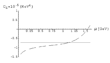
Figure 1: Plot of the total contribution to $C_{Z}$, Eqs. (41) plus (2), i) when only Goldstones are considered in Eq. (2) (dashed curve), ii) full result including all terms in Eq. (2) with just one vector and axial-vector resonances (solid curve).

In Fig. 1 we compare the complete result (with just one resonance for the vector and axial-vector channels) with the value obtained for $C_{Z}$ when only Goldstones are included in the long-distance part, i.e. only the first two terms of Eq. (2) are kept. One immediately sees that the complete result shows a flat dependence on the cutoff $\mu$, as it should, while the result with only Goldstones shows a certain dependence on $\mu$. One also sees that for a reasonable value of the cutoff $\mu\sim 1.15$ GeV (which is some sort of average between the $\rho$ and $a_{1}$ masses) the result with only Goldstones gives the right answer but that, if one misses the right value of $\mu$ in this guess, one can easily even flip the sign of the whole contribution.

We think this clearly exemplifies the potential dangers of a calculation with only Goldstones and a physical Euclidean cutoff [12][15].

3 ELECTROWEAK PENGUIN OPERATORS

Within the framework discussed above, we have also shown [16] that the $K\to\pi\pi$ matrix elements of the four-quark operator,

$$Q_{7}=6(\bar{s}_{L}\gamma^{\mu}d_{L})\sum_{q=u,d,s}e_{q}(\bar{q}_{R}\gamma_{\mu}q_{R})\,,$$ (43)

can be calculated to first non–trivial order in the chiral expansion and in the $1/N_{C}$ expansion.

The operator $Q_{7}$ emerges at the $M_{W}$ scale from considering the so-called electroweak penguin diagrams. In the presence of the strong interactions, the renormalization group evolution of $Q_{7}$ from the scale $M_{W}$ down to a scale $\mu{\ \lower-1.2pt\vbox{\hbox{\hbox to0.0pt{$<$\hss}\lower 5.0pt\vbox{\hbox{$\sim$}}}}\ }m_{c}$ mixes this operator with others, in particular with the four-quark density-density operator $Q_{8}$

$$Q_{8}=-12\sum_{q=u,d,s}e_{q}(\bar{s}_{L}q_{R})(\bar{q}_{R}d_{L})\,.$$ (44)

These two operators, times their corresponding Wilson coefficients, contribute to the lowest order ${\cal O}(p^{0})$ effective chiral Lagrangian which induces $|\Delta S|=1$ transitions in the presence of electromagnetic interactions to order ${\cal O}(\alpha)$ and of virtual $Z^{0}$ exchange, i.e., the Lagrangian [17]

$${\cal L}_{\chi,0}^{|\Delta S|=1}=-\frac{G_{\mbox{\rm{\tiny F}}}}{\sqrt{2}}\frac{\alpha}{\pi}V_{ud}V_{us}^{\ast}\times$$

$$\frac{M_{\rho}^{6}}{16\pi^{2}}\,\mbox{\bf h}\,\mbox{\rm tr}\left(U\lambda_{L}^{(23)}U^{\dagger}Q_{R}\right)+\mbox{\rm h.c.}\,,$$ (45)

where $\lambda_{L}^{(23)}$ is the effective left–handed flavour matrix $\left(\lambda_{L}^{(23)}\right)_{ij}=\delta_{i2}\delta_{3j}$ $(i,j=1,2,3)$. This is the only possible invariant which in the Standard Model can generate $|\Delta S|=1$ transitions to orders ${\cal O}(\alpha)$ and ${\cal O}(p^{0})$ in the chiral expansion. The coupling constant h is dimensionless and, a priori, of order ${\cal O}(N_{C}^{2})$ in the $1/N_{C}$ expansion. It plays a crucial rôle in the phenomenological analysis of radiative corrections to the $K\rightarrow\pi\pi$ amplitudes, hence the interest of identifying all the possible contributions to this constant.

The bosonization of the operator $Q_{7}$ to next-to-leading order in the $1/N_{C}$ expansion turns out to be entirely analogous to the bosonization of the operator $Q_{LR}\equiv\left(\bar{q}_{L}\gamma^{\mu}Q_{L}q_{L}\right)\left(\bar{q}_{R}\gamma^{\mu}Q_{R}q_{R}\right)$ which governs the electroweak $\pi^{+}\!-\!\pi^{0}$ mass difference discussed in the previous section. Because of the $LR$ structure, the factorized component of $Q_{7}$, which is leading in $1/N_{C}$, cannot contribute to the ${\cal O}(p^{0})$ low-energy effective Lagrangian in Eq. (3). The first ${\cal O}(p^{0})$ contribution from this operator is next-to-leading in the $1/N_{C}$ expansion and is given by the integral [16],

$$Q_{7}\rightarrow-3ig_{\mu\nu}\int\frac{d^{4}q}{(2\pi)^{4}}\Pi_{LR}^{\mu\nu}(q)\times$$

$$\mbox{\rm tr}\left(U\lambda_{L}^{(23)}U^{\dagger}Q_{R}\right)\,,$$ (46)

involving the same two-point function as in Eq. (8). This integral, however, is divergent for large $Q^{2}$ and needs to be regulated. The usual prescription [12] for the evaluation of integrals such as this, consists in taking a sharp cut-off in the (Euclidean) integration over $Q^{2}$,

$$Q_{7}\rightarrow-6\frac{3}{32\pi^{2}}\int_{0}^{\Lambda^{2}}dQ^{2}Q^{2}\left(-Q^{2}\Pi_{LR}(Q^{2})\right)\times$$

$$\!\!\!\!\!\mbox{\rm tr}\left(U\lambda_{L}^{(23)}U^{\dagger}Q_{R}\right)\,.$$ (47)

Inserting the same large–$N_{C}$ expression for the function $\Pi_{LR}(Q^{2})$ as in Eq. (1), with the short–distance constraints between the couplings and masses of the narrow states incorporated, the integral on the r.h.s. of Eq. (3) becomes then only logarithmically dependent on the ultraviolet scale $\Lambda$, and one obtains the following result

$$\int_{0}^{\Lambda^{2}}dQ^{2}Q^{2}\left(-Q^{2}\Pi_{LR}(Q^{2})\right)=$$

$$\sum_{A}f_{A}^{2}M_{A}^{6}\log\frac{\Lambda^{2}}{M_{A}^{2}}-\sum_{V}f_{V}^{2}M_{V}^{6}\log\frac{\Lambda^{2}}{M_{V}^{2}}\,,$$ (48)

for values of the cutoff much larger than any resonance mass included in the difference. Notice that if only the contribution from the Goldstone pole had been taken into account, the resulting expression would have displayed a polynomial dependence on the cut-off scale $\Lambda$. Another possibility is to evaluate the integral in Eq. (3) within a dimensional regularization scheme, say ${\overline{MS}}$, in which case one obtains the same result as in Eq. (3), but with the correspondence between the cut–off $\Lambda$ and the ${\overline{MS}}$ subtraction scale $\mu$ given by $\Lambda=\mu\cdot e^{\frac{1}{6}}$. In this case we can check that our result satisfies the correct renormalization group equation, i.e. by acting with $\mu d/d\mu$ on $Q_{7}$ in Eqs. (3,3) one obtains

$$\mu\frac{d}{d\mu}Q_{7}=\frac{-9}{8\pi^{2}}\left(\sum_{A}f_{A}^{2}M_{A}^{6}-\sum_{V}f_{V}^{2}M_{V}^{6}\right)$$

$$\times\mbox{\rm tr}\left(U\lambda_{L}^{(23)}U^{\dagger}Q_{R}\right)$$

$$=\frac{6}{4\pi}\alpha_{s}Q_{8}\,,\qquad\qquad\qquad$$ (49)

where one has to bosonize the operator $Q_{8}$ in Eq. (44) utilizing, mutatis mutandis, the rule of Eq. (2) and the constraint of Eq. (2).

The bosonic expression of $Q_{7}$ given by Eqs. (3) and (3) enables us to compute the $K\to\pi\pi$ matrix elements induced by this operator which, following the usual conventions, we express in terms of the following isospin amplitudes

$$\langle Q_{7}\rangle_{I}\equiv\langle(\pi\pi)_{I}|Q_{7}|K^{0}\rangle\,,\qquad I=0,2\,.$$ (50)

To leading order ${\cal O}(p^{0})$ in the chiral expansion and to next–to–leading order in the $1/N_{C}$ expansion, ${\cal O}(1/\sqrt{N_{C}})$ for $K\rightarrow\pi\pi$ amplitudes, we obtain the result

$$\langle Q_{7}\rangle_{0}=\sqrt{2}\langle Q_{7}\rangle_{2}=\frac{6\sqrt{3}}{16\pi^{2}F_{0}^{3}}\times$$ (51)

$$\!\!\!\!\!\!\!\!\!\!\!\left(\sum_{A}f_{A}^{2}M_{A}^{6}\log\frac{\Lambda^{2}}{M_{A}^{2}}-\sum_{V}f_{V}^{2}M_{V}^{6}\log\frac{\Lambda^{2}}{M_{V}^{2}}\right)\,.$$

It has become customary to parameterize the results of weak matrix elements of four-quark operators $Q_{i}$ in terms of the factorized contributions from the so-called vacuum saturation approximation, modulated by correction factors, the so called $B$–factors. Although the resulting $B$ factors for the $\Delta I=1/2$ and $\Delta I=3/2$ transitions generated by the $Q_{7}$ operator are found to depend only logarithmically on the matching scale $\mu$, their actual numerical values turn out to be rather sensitive to the precise choice of $\mu$ in the GeV region. Furthermore, because of the normalization to the vacuum saturation approximation inherent to the (rather disgraceful) conventional definition of $B$-factors, there appears a spurious dependence on the light quark masses as well. In Fig. 2 we show our prediction for the ratio

$${\widetilde{B}}_{7}^{(3/2)}\,\equiv\,\frac{\langle\pi^{+}|Q_{7}^{(3/2)}|K^{+}\rangle}{\langle\pi^{+}|Q_{7}^{(3/2)}|K^{+}\rangle^{\rm VSA}_{0}}\,,$$ (52)

versus the matching scale $\mu$ defined in the ${\overline{MS}}$ scheme. This is also the ratio considered in recent lattice QCD calculations [18]. [In fact, the lattice definition of ${\widetilde{B}}_{7}^{(3/2)}$ uses a current algebra relation between the $K\to\pi\pi$ and the $K\to\pi$ matrix elements which is only valid at order ${\cal O}(p^{0})$ in the chiral expansion.] In Eq. (52), the matrix element in the denominator is evaluated in the chiral limit, as indicated by the $0$ subscript .

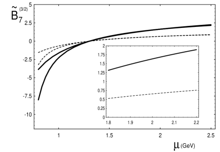
Figure 2: The $\tilde{B}_{7}^{(3/2)}$ factor in Eq. (52) versus $\mu$ in GeV. Solid lines correspond to $(m_{s}\!+\!m_{d})(2\,{\rm GeV})=158\,{\rm MeV}$; dashed lines to $(m_{s}+m_{d})(2\,{\rm GeV})=100\,{\rm MeV}$.

It would be much better, whenever possible, to compare lattice results directly of the amplitude $\langle\pi^{+}|Q_{7}^{(3/2)}|K^{+}\rangle$ with our prediction

$$\langle\pi^{+}|Q_{7}^{(3/2)}|K^{+}\rangle=\frac{3}{8\pi^{2}F_{0}^{2}}\!\left[\!\sum_{A}\!\!f_{A}^{2}M_{A}^{6}\log\frac{M_{A}^{2}}{\Lambda^{2}+M_{A}^{2}}\right.$$ (53)

$$\left.-\sum_{V}f_{V}^{2}M_{V}^{6}\log\frac{M_{V}^{2}}{\Lambda^{2}+M_{V}^{2}}\right]\simeq$$

$$\!\!\!\!\!\!\!\!\frac{3M_{V}^{4}}{4\pi^{2}}\left(\log\frac{\Lambda^{2}+M_{V}^{2}}{M_{V}^{2}}-2\log\frac{\Lambda^{2}+2M_{V}^{2}}{2M_{V}^{2}}\right)\,,$$

where in the second line we have used the LMD approximation discussed in Ref. [9], or the equivalent expression in the ${\overline{MS}}$ regularization, namely,

$$\langle\pi^{+}|Q_{7}^{(3/2)}(\mu)|K^{+}\rangle|_{\mbox{\rm}{\overline{MS}}}=$$ (54)

$$\frac{3M_{V}^{4}}{4\pi^{2}}\left(2\log 2-\log\frac{\mu^{2}e^{1/3}}{M_{V}^{2}}\right)\,.$$

Numerically one obtains $-0.02\pm 0.01$ GeV⁴ for the expression in Eq. (54) evaluated at $\mu=2$ GeV. The error is an estimate of $1/N_{C}$ corrections and corrections to the LMD limit.

It is interesting to compare the $\Lambda$ dependence of Eq. (53) with the $\mu$ dependence of Eq. (54). The two results clearly coincide for asymptotic values of their respective $\Lambda$ and $\mu$ scales. The situation, however, is rather different for values of these scales in the GeV region. This can be best seen by looking at the functional relation between these two scales which follows from identifying the two expressions in Eqs. (53) and (54): setting $x\equiv\frac{\mu^{2}}{M_{V}^{2}}e^{1/3}$ and $y\equiv\frac{\Lambda^{2}}{M_{V}^{2}}$ this relation is given by the function $x=4\frac{(1+y/2)^{2}}{1+y}$. The requirement that $y\geq 0$ results in a non trivial constraint $x\geq 4$, i.e., $\mu\geq 2e^{-1/6}M_{V}=1.69M_{V}$. In fact, at the value $\mu=1.69M_{V}$ the matrix element in Eq. (54) flips its sign in contradiction with a general positivity property [19] which demands that $-Q^{2}\Pi(Q^{2})\geq 0$ for all values of $0\leq Q^{2}\leq\infty$. Although the specific critical value $\mu=1.69M_{V}$ depends on the hadronic LMD approximation which we have made, it shows that pushing the matching of four-quark operators at low $\mu^{2}$ values in the ${\overline{MS}}$ regularization scheme may be very dangerous and can lead to totally misleading results.

4 DECAY OF PSEUDOSCALARS INTO LEPTON PAIRS

The examples discussed so far involved only the two-point function $\Pi_{LR}$. In this section we present an example which allows us to study the matching between short and long distances in the case where a three-point function is involved [20]. The physical processes of interest are the decay of $\pi^{0}$ or $\eta$ into a pair of charged leptons. These processes are dominated by the exchange of two virtual photons, as shown in Fig. 3, and it is therefore phenomenologically useful to consider the branching ratios normalized to the two-photon branching ratio ($P=\pi^{0},\eta$)

$$\!\!\!\!\!\!\!\!\!\!R(P\to\ell^{+}\ell^{-})=\frac{Br(P\to\ell^{+}\ell^{-})}{Br(P\to\gamma\gamma)}$$

$$\qquad=2\bigg{(}\frac{\alpha m_{\ell}}{\pi M_{P}}\bigg{)}^{2}\,\beta_{\ell}(M_{P}^{2})\,|{\cal A}(M_{P}^{2})|^{2},$$ (55)

with $\beta_{\ell}(s)=\sqrt{1-4m_{\ell}^{2}/s}$. The unknown dynamics is then contained in the amplitude ${\cal A}(M_{P}^{2})$. To lowest order in the chiral expansion the contribution to this amplitude arises from the two graphs of Fig. 3 with the result

$$\!\!\!\!{\cal A}(s)=\chi_{P}(\mu)+\frac{N_{C}}{3}\bigg{[}\,-\frac{5}{2}$$

$$\qquad+\frac{3}{2}\ln\bigg{(}\frac{m_{\ell}^{2}}{\mu^{2}}\bigg{)}\,+\,C(s)\,\bigg{]},$$ (56)

where

$$\chi_{\pi^{0}}=\chi_{\eta}=-\frac{(\chi_{1}+\chi_{2})}{4}\equiv\chi\quad,$$ (57)

with $\chi_{1}$ and $\chi_{2}$ the couplings of the two counterterms which describe the direct interactions of pseudoscalar mesons with lepton pairs to lowest order in the chiral expansion [21]

$$\!\!\!\!\!\!\!{\cal L}_{P\ell^{+}\ell^{-}}=\frac{3i}{32}\left(\frac{\alpha}{\pi}\right)^{2}\,{\bar{\ell}}\gamma^{\mu}\gamma_{5}\ell$$

$$\!\!\!\!\!\times\,\big{[}\chi_{1}\mbox{\rm tr}(Q_{R}Q_{R}D_{\mu}UU^{\dagger}-Q_{L}Q_{L}D_{\mu}U^{\dagger}U)$$

$$\!\!\!\!\!+\,\chi_{2}\mbox{\rm tr}(U^{\dagger}Q_{R}D_{\mu}UQ_{L}-UQ_{L}D_{\mu}U^{\dagger}Q_{R})\big{]}.$$ (58)

The function $C(s)$ in Eq. (56) corresponds to a finite three–point loop integral which can be expressed in terms of the dilogarithm function ${\mbox{Li}}_{2}(x)\,=\,-\int_{0}^{x}(dt/t)\ln(1-t)$. For $s<0$, its expression reads

$$C(s) = \frac{1}{\beta_{\ell}(s)}\bigg{[}\,{\mbox{Li}}_{2}\bigg{(}\frac{\beta_{\ell}(s)-1}{\beta_{\ell}(s)+1}\bigg{)}\,+\,\frac{\pi^{2}}{3}$$ (59)

$$+\,\frac{1}{4}\ln^{2}\bigg{(}\frac{\beta_{\ell}(s)-1}{\beta_{\ell}(s)+1}\bigg{)}\,\bigg{]}.$$

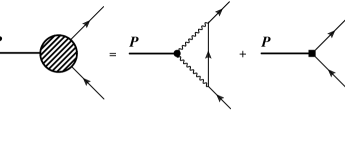
Figure 3: The lowest order contributions to the $P\to\ell^{+}\ell^{-}$ decay amplitude. The second graph denotes the contribution from the counterterm Lagrangian of Eq. (58).

The corresponding expression for $s>4m_{\ell}^{2}$ is obtained by analytic continuation, using the usual $i\epsilon$ prescription. The loop diagram of Fig. 3 originates from the usual coupling of the light pseudoscalar mesons to a photon pair given by the well–known Wess–Zumino anomaly [22]. The divergence associated with this diagram has been renormalized within the ${\overline{\mbox{MS}}}$ minimal subtraction scheme of dimensional regularization. The logarithmic dependence on the renormalization scale $\mu$ displayed in the above expression is compensated by the scale dependence of the combination $\chi(\mu)$ of renormalized low-energy constants defined above. Let us stress here that, as shown explicitly in Eq. (56) and in contrast with the usual situation in the purely mesonic sector, this scale dependence is not suppressed in the large–$N_{C}$ limit, since it does not arise from meson loops.

As a first step towards its subsequent evaluation we shall identify the coupling constant $\chi$ in terms of a QCD correlation function. For that purpose, consider the matrix element of the light quark isovector pseudoscalar density $P^{3}(x)\,=\,{1\over 2}({\bar{u}}i\gamma_{5}u-{\bar{d}}i\gamma_{5}d)(x)$ between leptonic states in the chiral limit. In the absence of weak interactions, and to lowest non-trivial order in the fine structure constant, this matrix element is given by the integral

$$\!\!\!\!\!\!\!\!<\ell^{-}(p^{\prime})\,|\,P^{3}(0)\,|\,\ell^{-}(p)>\qquad$$

$$=e^{4}\int\frac{d^{4}q}{(2\pi)^{4}}\,\frac{{\bar{u}}(p^{\prime})\gamma^{\mu}[{\not\!p}^{\prime}-{\not\!q}+m_{\ell}]\gamma^{\nu}u(p)}{[(p^{\prime}-q)^{2}-m_{\ell}^{2}]q^{2}(p^{\prime}-p-q)^{2}}$$

$$\quad\times\,i\int d^{4}x\int d^{4}y\,e^{iq\cdot x}e^{i(p^{\prime}-p-q)\cdot y}$$

$$\quad\times<0\,|\,T\{j_{\mu}^{\mbox{\scriptsize{em}}}(x)j_{\nu}^{\mbox{\scriptsize{em}}}(y)P^{3}(0)\}\,|\,0>,$$ (60)

with $j_{\mu}^{\mbox{\scriptsize{em}}}={1\over 3}(2{\bar{u}}\gamma_{\mu}u-{\bar{d}}\gamma_{\mu}d-{\bar{s}}\gamma_{\mu}s)$. In the chiral limit, the QCD three–point correlator appearing in this expression is again an order parameter of spontaneous chiral symmetry breaking. Bose symmetry and parity conservation of the strong interactions yield

$$\!\!\!\!\!\!\!\!\!\!\int d^{4}x\int d^{4}y\,e^{iq_{1}\cdot x}e^{iq_{2}\cdot y}$$

$$\times<0\,|\,T\{j_{\mu}^{\mbox{\scriptsize{em}}}(x)j_{\nu}^{\mbox{\scriptsize{em}}}(y)P^{3}(0)\}\,|\,0>$$

$$=\ \frac{2}{3}\,\epsilon_{\mu\nu\alpha\beta}q_{1}^{\alpha}q_{2}^{\beta}\,{\cal H}(q_{1}^{2},q_{2}^{2},(q_{1}+q_{2})^{2}),$$ (61)

with ${\cal H}(q_{1}^{2},q_{2}^{2},(q_{1}+q_{2})^{2})={\cal H}(q_{2}^{2},q_{1}^{2},(q_{1}+q_{2})^{2})$. For very large (Euclidian) momenta, the leading short-distance behaviour of this correlation function is given by

$$\!\!\!\!\lim_{\lambda\to\infty}\,{\cal H}\big{(}(\lambda q_{1})^{2},(\lambda q_{2})^{2},(\lambda q_{1}+\lambda q_{2})^{2}\big{)}$$

$$=\ -\frac{1}{2\lambda^{4}}<{\bar{\psi}}\psi>\,\frac{q_{1}^{2}+q_{2}^{2}+(q_{1}+q_{2})^{2}}{q_{1}^{2}q_{2}^{2}(q_{1}+q_{2})^{2}}$$

$$\,+\,{\cal O}\bigg{(}\frac{\alpha_{s}}{\lambda^{4}},\frac{1}{\lambda^{6}}\bigg{)}.$$ (62)

Actually, what matters for the convergence of the integral in Eq. (60) is the leading short-distance singularity of the $T-$product of the two electromagnetic currents, which corresponds to

$$\!\!\!\!\!\!\!\!\lim_{\lambda\to\infty}\,{\cal H}\big{(}(\lambda q)^{2},(p^{\prime}-p-\lambda q)^{2},(p^{\prime}-p)^{2}\big{)}$$

$$=\ -\frac{1}{\lambda^{2}}<{\bar{\psi}}\psi>\,\frac{1}{q^{2}(p^{\prime}-p)^{2}}$$

$$+\,{\cal O}\bigg{(}\frac{\alpha_{s}}{\lambda^{2}},\frac{1}{\lambda^{3}}\bigg{)},$$ (63)

Thus, the loop integral in Eq. (60) is indeed convergent. The QCD corrections of order ${\cal O}(\alpha_{s})$ in Eqs. (26) and (63) will not be considered here. Let us however notice that since the pseudoscalar density $P^{3}(x)$ and the single-flavour $<{\bar{\psi}}\psi>$ condensate share the same anomalous dimension, the power-like fall-off displayed by Eqs. (26) and (63) is canonical, i.e. it is not modified by powers of logarithms of the momenta.

At very low momentum transfers, the same correlator can be computed within Chiral Perturbation Theory (ChPT). At lowest order, it is saturated by the pion-pole contribution, given by the anomalous coupling of a neutral pion, emitted by the pseudoscalar source $P^{3}(0)$, to the two electromagnetic currents, i.e.

$${\cal H}(0,0,(q_{1}+q_{2})^{2}) = \,\frac{N_{C}}{8\pi^{2}}\,\frac{<{\bar{\psi}}\psi>}{F_{0}^{2}}\,\frac{1}{(q_{1}+q_{2})^{2}}$$ (64)

$$+\cdots\ ,$$

where the ellipsis stands for higher orders in the low-momentum expansion. The matrix element $<\ell^{-}(p^{\prime})\,|\,P^{3}(0)\,|\,\ell^{-}(p)>$ itself may also be evaluated in ChPT. At lowest order, it is given by the diagrams of Fig. 3, where the (off-shell) pion is now emitted by the pseudoscalar source $P^{3}(0)$. The result reads, with $t=(p^{\prime}-p)^{2}$,

$$\!\!\!\!\!\!\!\!<\ell^{-}(p^{\prime})\,|\,P^{3}(0)\,|\,\ell^{-}(p)>\big{|}_{\mbox{~{}\scriptsize{ChPT}}}$$ (65)

$$=\ -\frac{ie^{4}}{32\pi^{4}t}\,\frac{<{\bar{\psi}}\psi>}{F_{0}^{2}}\,m_{\ell}{\bar{u}}(p^{\prime})\gamma_{5}u(p)\,{\cal A}(t),$$

with the function ${\cal A}(t)$ defined in Eqs. (56) and (59). The contribution of the loop diagram of Fig. 3 is obtained upon replacing, in Eq. (60), the three-point QCD correlator by its lowest order chiral expression given in Eq. (64). The coupling constant $\chi(\mu)$ is thus given by the residue of the pole at $t=0$ of the matrix element $<\ell^{-}(p^{\prime})\,|\,P^{3}(0)\,|\,\ell^{-}(p)>$, after subtraction of the contribution of the two-photon loop, i.e.

$$\frac{\chi(\mu)}{32\pi^{4}}\,\frac{<{\bar{\psi}}\psi>}{F_{0}^{2}}\,m_{\ell}{\bar{u}}(p^{\prime})\gamma_{5}u(p)\qquad\qquad\qquad\qquad$$

$$=\ -\frac{2i}{3}\,{\bar{u}}(p^{\prime})\gamma_{\lambda}\gamma_{5}u(p)\qquad\times\qquad\qquad\qquad$$

$$\lim_{(p^{\prime}-p)^{2}\to 0}\int\frac{d^{d}q}{(2\pi)^{d}}\frac{(p^{\prime}-p)^{2}}{[(p^{\prime}-q)^{2}-m_{\ell}^{2}]q^{2}(p^{\prime}-p-q)^{2}}$$

$$\times\,(p^{\prime}-p-2q)_{\alpha}\bigg{[}\,q^{\alpha}(p^{\prime}-p)^{\lambda}-\,(p^{\prime}-p)^{\alpha}q^{\lambda}\,\bigg{]}$$

$$\!\!\!\!\times\,\bigg{[}\,{\cal H}(q^{2},(p^{\prime}-p-q)^{2},(p^{\prime}-p)^{2})$$

$$\!\!\!\!\quad-\,{\cal H}(0,0,(p^{\prime}-p)^{2})\,\bigg{]}.\quad$$ (66)

In the large-$N_{C}$ limit, the three–point correlator (4) is given by the tree–level exchanges of vector and pseudoscalar resonances, as shown in Fig. 4, so that the singularities in each channel consist of a succession of simple poles. This involves couplings of the resonances among themselves and to the external sources which, just like the masses of the resonances themselves, cannot be fixed in the absence of an explicit solution of QCD in the large-$N_{C}$ limit. Nevertheless, the general structure of the quantity appearing in Eq. (4) is of the form

$$\lim_{(p^{\prime}-p)^{2}\to 0}\,(p^{\prime}-p)^{2}\,{\cal H}(q^{2},q^{2},(p^{\prime}-p)^{2})=$$

$$\ -\frac{1}{2}\frac{<{\bar{\psi}}\psi>}{F_{0}^{2}}\qquad\qquad\qquad\qquad$$

$$\times\ \sum_{V}\,M_{V}^{2}\,\bigg{[}\,\frac{a_{V}}{(q^{2}-M_{V}^{2})}\,-\,\frac{b_{V}q^{2}}{(q^{2}-M_{V}^{2})^{2}}\,\bigg{]}\ ,$$ (67)

where a priori the sum extends over the infinite spectrum of vector resonances of QCD in the large-$N_{C}$ limit. Equation (4) follows from the fact that its left-hand side enjoys some additional properties: i) In the pseudoscalar channel, only the pion pole survives, while massive pseudoscalar resonances cannot contribute. ii) The momentum transfer in the two vector channels is the same. iii) Its high–energy behaviour is fixed by Eq. (63).

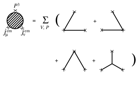
Figure 4: The contributions to the vector–vector–pseudoscalar three–point function in the large–$N_{C}$ limit of QCD. The sum extends over the infinite number of zero-width vector ($V$) and pseudoscalar ($P$) states.

Even though the constants $a_{V}$ and $b_{V}$ depend on the masses and couplings of the vector resonances in an unknown manner, they are however constrained by the two conditions

$$\sum_{V}\,a_{V}=\frac{N_{C}}{4\pi^{2}},\quad\sum_{V}\,(a_{V}\,-\,b_{V})\,M_{V}^{2}=2F_{0}^{2},$$ (68)

which follow from Eqs. (64) and (63), respectively. Notice that there are no contributions from the perturbative QCD continuum to these sums. Taking the first of these conditions (which, coming from the anomaly, has no ${\cal O}(\alpha_{s})$ corrections) into account, we obtain

$$\chi(\mu)=\frac{5N_{C}}{12}-2\pi^{2}\,\sum_{V}\,\bigg{[}\,a_{V}\ln\left(\frac{M_{V}^{2}}{\mu^{2}}\right)\,-\,b_{V}\,\bigg{]}.$$ (69)

This equation, together with the two conditions (68), constitutes the central result of Ref. [20]. This is as far as the large-$N_{C}$ limit allows us to go. Let us point out that the scale dependence of $\chi(\mu)$ is correctly reproduced by the expression (69), again as a consequence of the first condition in Eq. (68).

Within the LMD approximation of large–$N_{C}$ QCD, it is easy to write down the expression of the correlation function ${\cal H}(q_{1}^{2},q_{2}^{2},(q_{1}+q_{2})^{2})$ which correctly interpolates between the high energy behaviour in Eq. (26) and the ChPT result in Eq. (64) [23]

$${\cal H}^{\mbox{\scriptsize LMD}}(q_{1}^{2},q_{2}^{2},(q_{1}+q_{2})^{2})\ =\ -\frac{1}{2}<{\bar{\psi}}\psi>$$

$$\times\frac{q_{1}^{2}+q_{2}^{2}+(q_{1}+q_{2})^{2}-M_{V}^{4}a_{V}^{\mbox{\scriptsize LMD}}/F_{0}^{2}}{(q_{1}^{2}-M_{V}^{2})(q_{2}^{2}-M_{V}^{2})(q_{1}+q_{2})^{2}}.$$ (70)

Notice that this expression also correctly reproduces the behaviour in Eq. (63). In this approximation, the two conditions (68) completely pin down the two quantities $a_{V}$ and $b_{V}$ in terms of $F_{0}$ and of the mass $M_{V}$ of this lowest lying vector meson octet,

$$a_{V}^{\mbox{\scriptsize LMD}}=\frac{N_{C}}{4\pi^{2}}\quad\mbox{and}\quad b_{V}^{\mbox{\scriptsize LMD}}=\frac{N_{C}}{4\pi^{2}}\,-\,\frac{2F_{0}^{2}}{M_{V}^{2}}.$$ (71)

With the results of Eq. (71), and for $N_{C}$=3, it follows from Eq. (69) that

$$\chi^{\mbox{\scriptsize LMD}}(\mu)=\frac{11}{4}\,-\,\frac{3}{2}\ln\left(\frac{M_{V}^{2}}{\mu^{2}}\right)-4\pi^{2}\frac{F_{0}^{2}}{M_{V}^{2}}.$$ (72)

Numerically, using the physical values $F_{0}\simeq 87$ MeV and $M_{V}=M_{\rho}=770$ MeV, we obtain

$$\chi^{\mbox{\scriptsize LMD}}(\mu=M_{V})\ =\ 2.2\pm 0.9,$$ (73)

where we have allowed for a systematic theoretical error of 40%, as a rule of thumb estimate of the uncertainties attached to the large-$N_{C}$ and LMD approximations. The predicted ratios of branching ratios in Eq. (55) which follow from this result [26] are displayed in Table 1. We conclude that, within errors, the LMD–approximation to large-$N_{C}$ QCD reproduces well the observed rates of pseudoscalar mesons decaying into lepton pairs.

Table 1: The values for the ratios $R(P\to\ell^{+}\ell^{-})$ obtained within the LMD approximation to large–$N_{C}$ QCD and the comparison with available experimental results.

$R$	LMD	Experiment
$R(\pi^{0}\to e^{+}e^{-})\times 10^{8}$	$6.2\pm 0.3$	$7.13\pm 0.55$ [27]
$R(\eta\to\mu^{+}\mu^{-})\times 10^{5}$	$1.4\pm 0.2$	$1.48\pm 0.22$ [28]
$R(\eta\to e^{+}e^{-})\times 10^{8}$	$1.15\pm 0.05$	—

At first sight this approximation may resemble good old Vector Meson Dominance (VMD). However, there are important differences. Firstly, the systematic use of the $1/N_{C}$ expansion in QCD justifies the use of single particle intermediate states (and substantiates what otherwise is only an ansatz in VMD). And secondly, the use of the OPE resolves certain difficulties in the traditional VMD phenomenological approach, such as e.g. the ambiguity in the use of the VMD prescription for just one photon or for both photons in the decay $P\rightarrow\ell^{+}\ell^{-}$. This ambiguity is important, since making the wrong choice may result in a violation of the OPE constraints given by Eqs. (4,4) [29].

The situation in the case of the $|\Delta S|=1$ decay $K_{L}^{0}\to\ell^{+}\ell^{-}$ is slightly more delicate. It has recently been shown [30] that these processes can also be described by the expressions (55) and (56), but with an effective constant $\chi_{K^{0}_{L}}$ containing an additional piece from the short-distance contributions [31]. Of course, a cast-iron understanding of these transitions is very important [32] as the evaluation of $\chi(\mu)$ could then have a potential impact on possible constraints on physics beyond the Standard Model. At present, the most accurate experimental determination of the $K_{L}^{0}\to\mu^{+}\mu^{-}$ branching ratio [35] gives the result: $Br(K_{L}^{0}\to\mu^{+}\mu^{-})=(7.18\pm 0.17)\times 10^{-9}$. Using the experimental branching ratio [28] $Br(K_{L}^{0}\to\gamma\gamma)=(5.92\pm 0.15)\times 10^{-4}$, this leads to a unique solution for an effective $\chi_{K_{L}^{0}}=5.17\pm 1.13$. The authors of Ref. [30] argue that, to a good approximation, one has

$$\chi_{K_{L}^{0}}=\chi-\epsilon_{\gamma\gamma}\ \delta\chi_{SD}\,,$$ (74)

where $\chi$ is the constant defined in Eq. (57) and $\epsilon_{\gamma\gamma}$ is the sign of the on-shell form factor $c(0,0)$ (for the notation, we refer to [30]; see in particular Eqs. (6) and (7) of that reference) describing the $K_{L}^{0}\to\gamma\gamma$ decay. However, as also discussed in Ref. [30], the decay $K_{L}\rightarrow\gamma\gamma$ itself is rather problematic. The problem comes from the fact that at lowest order in the $SU(3)_{L}\times SU(3)_{R}$ chiral expansion, one obtains $c(0,0)=0$. There are two ways to bypass this situation, either by considering higher orders, or by including the $\eta^{\prime}$ as an explicit degree of freedom already at leading order, which can be done within the framework of the $U(3)_{L}\times U(3)_{R}$ combined chiral and large-$N_{C}$ expansions along the lines suggested in Refs. [36]. In both cases, additional contributions to the counterterm Lagrangian in (58), and thus to the effective constant $\chi_{K_{L}^{0}}$, have to be considered: quark mass corrections in the first case, $1/N_{C}$ corrections in the second. To the best of our knowledge, an accurate estimate of either of these corrections has, unfortunately, not been attempted so far. The analysis in the $U(3)_{L}\times U(3)_{R}$ framework performed in Ref. [30] obtains the value of $c(0,0)$ from the experimental number for $K_{L}\rightarrow\gamma\gamma$ and determines its sign, on combined large-$N_{C}$ and phenomenological grounds, to be positive. In a large-$N_{C}$ calculation this experimental value for $c(0,0)$ would require going beyond the leading term because in the strict limit $N_{C}\rightarrow\infty$ — keeping $m_{u}=m_{d}=0,m_{s}\not=0$ for simplicity— one finds again $c(0,0)=0$. Consistency demands, then, that subleading terms be also included in the counterterms which contribute to $\chi_{K_{L}^{0}}$, something that goes beyond the scope of this work [37]. If, on the other hand, one accepts the plausible phenomenological arguments of Ref. [30] whereby these subleading terms are neglected, our result (73) leads then to $\chi_{K_{L}^{0}}=0.4\pm 1.1$, corresponding to a ratio $R(K_{L}^{0}\to\mu^{+}\mu^{-})=(2.24\pm 0.41)\times 10^{-5}$ which is $2.5\sigma$ above the experimental value $R(K_{L}^{0}\to\mu^{+}\mu^{-})=(1.21\pm 0.04)\times 10^{-5}$.

Acknowledgements

We thank Ll. Ametller, J. Bijnens, V. Giménez, J.I. Latorre, L. Lellouch, A. Pich and J. Prades for discussions and M. Perrottet for a very pleasant collaboration.

Work supported in part by TMR, EC-Contract No. ERBFMRX-CT980169 (EURODA$\phi$NE). The work of S.P. has also been partially supported by research project CICYT-AEN98-1093.

References

- [1] For a review, see D. Treille, in probing the Standard Model of particle interactions, Les Houches Summer School 1997, R. Gupta et al. eds., North Holland (1999).
- [2] See for instance A.J. Buras in [1] and references therein.
- [3] J. Gasser and H. Leutwyler, Nucl. Phys. B250 (1985) 465.
- [4] J. Gasser and H. Leutwyler, Ann. Phys. (N.Y.) 158 (1984) 142.
- [5] M. Knecht and E. de Rafael, Phys. Lett. B424 (1998) 335.
- [6] T. Das et al., Phys. Rev. Lett. 18 (1967) 759.
- [7] W.A. Bardeen, J. Bijnens and J.-M. Gérard, Phys. Rev. Lett. 62 (1989) 1343.
- [8] S. Weinberg, Phys. Rev. Lett. 18 (1967) 507.
- [9] S. Peris, M. Perrottet and E. de Rafael, JHEP 05 (1998) 011; M. Golterman and S. Peris, hep-ph/9908252.
- [10] M. Knecht, S. Peris and E. de Rafael, Phys. Lett.B443 (1998) 255.
- [11] E. de Rafael, “Chiral Lagrangians and Kaon CP–Violation”, in CP Violation and the Limits of the Standard Model, Proc. TASI’94, ed. J.F. Donoghue (World Scientific, Singapore, 1995).
-
[12]
W.A. Bardeen, A.J. Buras and J.-M. Gérard, Nucl. Phys. B293
(1987) 787; Phys. Lett. B192 (1987) 138;
B211 (1988) 343.
W.A. Bardeen, J. Bijnens and J.-M. Gérard, Phys. Rev. Lett. 62 (1989) 1343.
For a review and further references, see A.J. Buras, “The 1/N Approach to Non-leptonic Weak Interactions”, in CP Violation, ed. C. Jarlskog (World Scientific, Singapore, 1989). - [13] J. Bijnens, J.-M. G érard and G. Klein, Phys. Lett. B257 (1991)191.
- [14] J.P. Fatelo and J.-M. G érard, Phys. Lett. B347 (1995) 136.
- [15] T. Hambye, G.O. Kohler and P.H. Soldan, Eur. Phys. J. C10 (1999) 271; T. Hambye, G.O. Kohler, E.A. Paschos and P.H. Soldan, hep-ph/9906434; T. Hambye and P.H. Soldan, hep-ph/9908232; T. Hambye, G.O. K öhler, E.A. Paschos, P.H. Soldan and W.A. Bardeen, Phys. Rev. D58 (1998) 014017; T. Hambye, Acta Phys. Pol. B28 (1997) 2479, and hep-ph/9806204; G. O. K öhler, hep-ph/9806224.
- [16] M. Knecht, S. Peris and E. de Rafael, Phys. Lett.B457 (1999) 277.
- [17] J. Bijnens and M. Wise, Phys. Lett. 137B (1984) 245.
- [18] L. Conti et al., Phys. Lett. B421, 273 (1998); C.R. Allton et al., hep-lat/9806016; L. Lellouch and C.-J. David Lin, hep-lat/9809142.
- [19] E. Witten, Phys. Rev. Lett. 51 (1983) 2351.
- [20] M. Knecht, S. Peris, M. Perrottet and E. de Rafael, hep-ph/9908283.
- [21] M.J. Savage, M. Luke and M.B. Wise, Phys. Lett.B291, 481 (1992).
- [22] J. Wess and B. Zumino, Phys. Lett. B37 95 (1971).
- [23] A similar analysis for the vector–vector–scalar and vector–axial–pseudoscalar three–point functions can be found in Refs. [24] and [25], respectively.
- [24] B. Moussallam and J. Stern, in Two - Photon Physics: From DAPHNE to LEP 200 and Beyond, edited by F. Kapusta and J.J. Parisi, World Scientific (1994), and hep-ph/9404353.
- [25] B. Moussallam, Nucl. Phys. B504, 381 (1997).
- [26] In the case of the decay into a muon pair, corrections lower the result of Eq. (73) by about 7%, and are taken into account in the numerical values of Table I.
- [27] A. Alavi-Harati et al., hep-exp/9903007 and references therein.
- [28] C. Caso et al., Review of Particle Physics, Eur. Phys. J. C3 1 (1998), and references therein.
- [29] See, for instance, Ll. Ametller, A. Bramon and E. Masso, Phys. Rev. D48 (1993) 3388 and references therein.
- [30] D. G ómez Dumm and A. Pich, Phys. Rev. Lett. 80, 4633 (1998).
- [31] G. Buchalla and A.J. Buras, Nucl. Phys. B412, 106 (1994); A.J. Buras and R. Fleischer, in Heavy Flavours II, edited by A.J. Buras and M. Linder, hep-ph/9704376.
- [32] We refer the reader to Ref. [30] for further details. See also Refs. [33] and [34] for an alternative approach.
- [33] G. D’Ambrosio, G. Isidori and J. Portol és, Phys. Lett. B423, 385 (1998).
- [34] G. Valencia, Nucl. Phys. B517, 339 (1998).
- [35] D. Ambrose et al., reported at the KAON’99 Workshop, Chicago, June 1999, (to be published).
- [36] P. Herrera-Siklody, J.I. Latorre, P. Pascual and J. Taron, Nucl. Phys. B497 (1997) 345; Phys. Lett. B419 (1998) 326; H. Leutwyler, Nucl. Phys. Proc. Suppl. 64 (1998) 223; R. Kaiser and H. Leutwyler, hep-ph/9806336.
- [37] See G.M. Shore and G. Veneziano, Nucl. Phys. B381 (1992) 3, for a discussion of the difficulties one encounters already in .