The possible form of New Physics (NP) interactions affecting the $ZZZ$, $ZZ\gamma$ and $Z\gamma\gamma$ vertices, is critically examined. Their signatures and the possibilities to study them, through $ZZ$ and $Z\gamma$ production, at the $e^{-}e^{+}$ Colliders LEP and LC and at the hadronic Colliders Tevatron and LHC, are investigated. Experimental limits obtained or expected on each coupling are collected. A simple theoretical model based on virtual effects due to some heavy fermions is used for acquiring some guidance on the plausible forms of these NP vertices. In such a case specific relations among the various neutral couplings are predicted, which can be experimentally tested and possibly used to constrain the form of the responsible NP structure.

1 Introduction

During the last two decades an intense activity has taken place about the possible existence of anomalous gauge boson couplings (i.e. non standard contributions). The general form of the 3-boson couplings was written, in a model-independent way, in terms of a set of seven independent Lorentz and $U(1)_{em}$ invariant operators[1, 2]. This general description has been applied to both charged ($\gamma WW$, $ZWW$) and neutral ($\gamma\gamma Z$, $\gamma ZZ$, $ZZZ$) sectors [2].

More recently, anomalous gauge boson couplings were considered in the framework of the Effective Lagrangians [3]. Here, the basic assumption is that, beyond SM, there exist new physics (NP) dynamics whose degrees of freedom are so heavy (of mass scale $\Lambda$) that they cannot be produced at present or near future colliders. The only observable effects should then be anomalous interactions of usual SM particles. Under these conditions, by integrating out these heavy NP states, the observable effects can be described by an Effective Lagrangian constructed in terms of operators involving only SM fields [2, 4]. So long as $\Lambda$ is much larger than the actually observable energy range, these operators are dominated by those with the lowest possible dimension. Each operator should be hermitian, multiplied by a constant coupling; while contributions from higher dimensional operators should be suppressed by powers of $s/\Lambda^{2}$.

The set of anomalous couplings can be classified and restricted using symmetry requirements and constraints on the highest allowed dimensionality. This procedure has been fruitfully applied to various sectors of the SM [5]. Thus, it has allowed to describe anomalous properties of several processes, like 4-fermion, 2 fermion-2 boson, 3-boson, 4-boson interactions; where the fermions are leptons or light or heavy quarks, while the bosons are $\gamma$, W, Z and Higgs.

The charged 3-boson sector has been explored in great detail with this method, both theoretically and experimentally [6, 7]. The general form with 7 types of couplings (4 CP-conserving and 3 CP-violating for the photon and separately for the $Z$ also), was shown to be reduced to only 5 independent couplings (3 CP-conserving and 2 CP-violating) if one restricts to $dim=6$ $SU(2)\times U(1)$ gauge invariant operators in the linear representation [8]. While, in the non-linear representation case (where no light Higgs boson exists), one finds that 4 independent CP conserving and 3 CP violating $SU(2)\times U(1)$ gauge invariant operators contribute to triple gauge couplings, at the level of $d_{chiral}=4$ [9]. Various other assumptions can also reduce the number of independent couplings [10].

Experimental constraints have already been established through $W^{+}W^{-}$ production at LEP2 and $W\gamma$, $WZ$ production at the TEVATRON, [11, 12, 13]. Relations between the coupling constants and the effective NP scale $\Lambda$ have also been established through unitarity relations; which allow to translate the upper limits on these couplings into lower limits for the effective scale $\Lambda$ [14]. Using this framework, a comparison of the experimental results already obtained or expected at future colliders in the various processes, should allow to establish interesting constraints on the possible structure of the NP interactions. At least it should show what is the SM sector that NP may affect, and what symmetry property it may preserve.

Our first aim in this paper is to explore if similar information could be obtained in the neutral 3-boson sector. Up to now, this sector has received less attention than the charged one. Probably this is because charged boson couplings already received tree level Standard Model (SM) contributions, whereas the neutral ones do not; so that they may be considered as purely ”anomalous”. The situation in it is less simple for several reasons. To the general Lorentz and $U(1)_{em}$ invariance requirements, one should add the constraints due to Bose statistics, as there are always at least two identical particles. This forbids $ZZZ$, $ZZ\gamma$ or $Z\gamma\gamma$ interactions vertices when all particles are on-shell [1]. The appearance of such vertices is only possible if at least one of the gauge bosons involved is off shell. The first discussions about these couplings were given in [15]. The most general allowed form involves only 2 independent couplings for each of the $VZZ$ vertices ($V=\gamma,~{}Z$; one CP-conserving and one CP-violating) and 4 independent couplings for each of the $VZ\gamma$ vertices ($V=\gamma,~{}Z$; two CP-conserving and two CP-violating). There is a priori no relation between these various couplings. Explicit expressions for these vertices were written in [2] and have then be widely used. However we noticed that a factor $i$ was omitted in the set of $VZ\gamma$ vertices. This factor $i$ is absolutely necessary in order the related effective New Physics (NP) Lagrangian to be hermitian.

As in the charged 3-boson sector, this effective lagrangian may be written in an $SU(2)\times U(1)$ invariant form. The only difference is that, while in the charged sector the NP interactions maybe generated already at the level of $dim=6$ operators; in the neutral sector we need operators of dimensions 8 or 10 in order for NP to be generated. So, if we restrict to $dim=6$ operators, no NP vertices in the neutral 3-boson sector is allowed. Thus, if such interactions exist, it would indicate either that some higher dimensional operators containing neutral 3-boson vertices without appreciable admixture from charged ones are somehow enhanced; or that the NP scale is rather nearby, so that there is no dimensional ordering on the size of the various operators. But of course, in such a case direct production of the new degrees of freedom may be observable. This fact should also arise when one tries to write unitarity constraints and relate the neutral couplings to the effective NP scale defined as the energy at which the various amplitudes saturate unitarity [14]. To be more precise we take one example of NP structure due to the one loop virtual effects of heavy fermions, and we discuss the corresponding pattern of anomalous couplings that are generated. It is found then the strength of these couplings may be enhanced compared to what the dimensionality of the related operators would had led us to expect. Moreover relations among the various couplings are obtained in such models. It will be very interesting to see what constraints the experimental measurements will put on these couplings; i.e. to see how they compare to the above theoretical pattern in the neutral and in the charged sectors.

Thus, our motivation for reconsidering the various $ZZ$ and $Z\gamma$ production processes at LEP2, LC, TEVATRON and LHC, is to see how they react to the presence of each of the anomalous couplings. In the next Section 2 we explicitly write the correct neutral 3-boson vertices and the Effective Lagrangian from which they derive. A toy model for the generation of such couplings is also presented. We then give the corresponding NP contributions to the helicity amplitudes for the $f\bar{f}\to ZZ,~{}Z\gamma$ processes. Our conventions are fully defined by the expressions for the SM parts of the amplitudes that we give in Appendix A. The expressions of the observables (cross sections and asymmetries) at the various colliders are given in Appendix B. In Section 3 we give explicit illustrations showing how the observables react to each of the anomalous couplings, in particular the interference patterns for the case of CP-conserving couplings. We emphasize the special role that longitudinal polarization would play at the LC Collider, for disentangling photon and $Z$ anomalous couplings. We also devote a special attention to the way these anomalous effects would be analyzed at hadron Colliders and the respective merits of transverse momentum, invariant mass and c.m. scattering angle distributions. Finally we summarize our observations and suggestions in Sect.4 .

2 Description of anomalous neutral boson couplings

Assuming only Lorentz and $U(1)_{em}$ gauge invariance as well as Bose statistics, the most general form of the $V_{1}V_{2}V_{3}$ vertex function defined in Fig.1, where $V_{1},V_{2}$ are on shell neutral gauge bosons, while $(V_{3}=Z~{},~{}\gamma)$ is in general off-shell but always coupled to a conserved current, has been given in [2]

$$\Gamma^{\alpha\beta\mu}_{ZZV}(q_{1},q_{2},P) = \frac{i(P^{2}-m_{V}^{2})}{m_{Z}^{2}}\left[f_{4}^{V}(P^{\alpha}g^{\mu\beta}+P^{\beta}g^{\mu\alpha})-f_{5}^{V}\epsilon^{\mu\alpha\beta\rho}(q_{1}-q_{2})_{\rho}\right]~{},$$ (1)

$$\Gamma^{\alpha\beta\mu}_{Z\gamma V}(q_{1},q_{2},P) = \frac{i(P^{2}-m_{V}^{2})}{m_{Z}^{2}}\Bigg{\{}h_{1}^{V}(q_{2}^{\mu}g^{\alpha\beta}-q_{2}^{\alpha}g^{\mu\beta})+\frac{h_{2}^{V}}{m_{Z}^{2}}P^{\alpha}[(Pq_{2})g^{\mu\beta}-q_{2}^{\mu}P^{\beta}]$$ (2)

$$- h_{3}^{V}\epsilon^{\mu\alpha\beta\rho}q_{2\rho}~{}-~{}\frac{h_{4}^{V}}{m_{Z}^{2}}P^{\alpha}\epsilon^{\mu\beta\rho\sigma}P_{\rho}q_{2\sigma}\Bigg{\}}~{}.$$

Compared to [2], we have introduced in (2) an additional factor $i$ in order for the related effective New Physics (NP) Lagrangian to be hermitian. Of course, the choice of the sign of this factor is a convention.

The effective Lagrangian generating the vertices (1, 2) is

$${\cal L}_{NP} = \frac{e}{m_{Z}^{2}}\Bigg{[}-[f_{4}^{\gamma}(\partial_{\mu}F^{\mu\beta})+f_{4}^{Z}(\partial_{\mu}Z^{\mu\beta})]Z_{\alpha}(\partial^{\alpha}Z_{\beta})+[f_{5}^{\gamma}(\partial^{\sigma}F_{\sigma\mu})+f_{5}^{Z}(\partial^{\sigma}Z_{\sigma\mu})]\widetilde{Z}^{\mu\beta}Z_{\beta}$$ (3)

$$- [h_{1}^{\gamma}(\partial^{\sigma}F_{\sigma\mu})+h_{1}^{Z}(\partial^{\sigma}Z_{\sigma\mu})]Z_{\beta}F^{\mu\beta}-[h_{3}^{\gamma}(\partial_{\sigma}F^{\sigma\rho})+h_{3}^{Z}(\partial_{\sigma}Z^{\sigma\rho})]Z^{\alpha}\widetilde{F}_{\rho\alpha}$$

$$- \left\{\frac{h_{2}^{\gamma}}{m_{Z}^{2}}[\partial_{\alpha}\partial_{\beta}\partial^{\rho}F_{\rho\mu}]+\frac{h_{2}^{Z}}{m_{Z}^{2}}[\partial_{\alpha}\partial_{\beta}(\square+m_{Z}^{2})Z_{\mu}]\right\}Z^{\alpha}F^{\mu\beta}$$

$$+ \left\{\frac{h_{4}^{\gamma}}{2m_{Z}^{2}}[\square\partial^{\sigma}F^{\rho\alpha}]+\frac{h_{4}^{Z}}{2m_{Z}^{2}}[(\square+m_{Z}^{2})\partial^{\sigma}Z^{\rho\alpha}]\right\}Z_{\sigma}\widetilde{F}_{\rho\alpha}\Bigg{]}~{},$$

where $\widetilde{Z}_{\mu\nu}=1/2\epsilon_{\mu\nu\rho\sigma}Z^{\rho\sigma}$ with $Z_{\mu\nu}=\partial_{\mu}Z_{\nu}-\partial_{\nu}Z_{\mu}$ and similarely for the photon tensor $F_{\mu\nu}$. The couplings $f_{4}^{V},~{}h_{1}^{V},~{}h_{2}^{V}$ violate CP invariance; while $f_{5}^{V},~{}h_{3}^{V},~{}h_{4}^{V}$ respect it.

The use of the equations of motion for the photon and Z-fields implies that the replacements

$$\partial^{\mu}F_{\mu\nu} \Longrightarrow eQ_{f}\bar{f}\gamma_{\nu}f~{},$$ (4)

$$\partial^{\mu}Z_{\mu\nu}+m_{Z}^{2}Z_{\nu} \Longrightarrow e\bar{f}\left(g^{Z}_{L}\gamma_{\nu}\frac{(1-\gamma_{5})}{2}~{}+~{}g^{Z}_{R}\gamma_{\nu}\frac{(1+\gamma_{5})}{2}\right)f~{},$$ (5)

$$(\square+m_{Z}^{2})Z_{\nu} \Longrightarrow e\bar{f}\left(g^{Z}_{L}\gamma_{\nu}\frac{(1-\gamma_{5})}{2}~{}+~{}g^{Z}_{R}\gamma_{\nu}\frac{(1+\gamma_{5})}{2}\right)f~{},$$ (6)

may be done in the first factor of each term in (3), where $f$ is any fermion with couplings defined in (A.4). Thus, the effective Lagrangian in (3) is essentially equivalent to a set of contact $f\bar{f}ZZ$ and $f\bar{f}Z\gamma$ interactions.

Of course, the computation of the NP scattering amplitudes for $f\bar{f}\to ZZ$ and $f\bar{f}\to Z\gamma$, either by using these contact interactions, or working directly with (3), gives the same results. They are given below, and should be added to the SM ones, which are due to fermion ($f$) exchange in the $t$-channel. These SM helicity amplitudes appear in Appendix A and serve to define our notations and conventions.

In $f\bar{f}\to ZZ$, the only non-vanishing NP helicity amplitudes induced by (1) are those where one $Z$ is transverse ($\tau_{1}\equiv\tau=\pm 1$) and the other longitudinal ($\tau_{2}=0$). In this case we have

$$F^{\lambda}_{\tau 0}(f\bar{f}\to ZZ~{};~{}NP)=F^{\lambda*}_{0,-\tau}(f\bar{f}\to ZZ~{};~{}NP)$$ (7)

$$= \frac{e^{2}\hat{s}^{3/2}\beta}{m_{Z}^{3}2\sqrt{2}}(1+\lambda\tau\cos\vartheta^{*})\left[i(f_{4}^{\gamma}Q_{f}+f_{4}^{Z}g_{\lambda}^{Z})-(f_{5}^{\gamma}Q_{f}+f_{5}^{Z}g_{\lambda}^{Z})\beta\tau\right]~{},$$

where the same definitions as in (A.7) are used.

Correspondingly for the NP contribution to $f\bar{f}\to Z\gamma$, compare (A.12)

$$F^{\lambda}_{\tau_{1}\tau_{2}}(f\bar{f}\to Z\gamma~{};~{}NP) = -~{}\frac{e^{2}(\hat{s}-m_{Z}^{2})\lambda}{4m_{Z}^{2}}\sin\vartheta^{*}\Big{[}i(h_{1}^{\gamma}Q_{f}+h_{1}^{Z}g_{\lambda}^{Z})(1+\tau_{1}\tau_{2})$$ (8)

$$-(\tau_{1}+\tau_{2})(h_{3}^{\gamma}Q_{f}+h_{3}^{Z}g_{\lambda}^{Z})\Big{]}~{}\mbox{ for }~{}\tau_{1}\tau_{2}\neq 0~{}~{},$$

$$F^{\lambda}_{0\tau_{2}}(f\bar{f}\to Z\gamma~{};~{}NP)=-~{}\frac{e^{2}\sqrt{\hat{s}}(\hat{s}-m_{Z}^{2})}{m_{Z}^{3}2\sqrt{2}}(1-\lambda\tau_{2}\cos\vartheta^{*})\Big{[}-i(h_{1}^{\gamma}Q_{f}+h_{1}^{Z}g_{\lambda}^{Z})$$

$$+i(h_{2}^{\gamma}Q_{f}+h_{2}^{Z}g_{\lambda}^{Z})\frac{(\hat{s}-m_{Z}^{2})}{2m_{Z}^{2}}+\tau_{2}(h_{3}^{\gamma}Q_{f}+h_{3}^{Z}g_{\lambda}^{Z})-\tau_{2}\frac{(\hat{s}-m_{Z}^{2})}{2m_{Z}^{2}}(h_{4}^{\gamma}Q_{f}+h_{4}^{Z}g_{\lambda}^{Z})\Big{]}~{},$$ (9)

where of course $\tau_{2}=\pm 1$.

A toy model: heavy fermion contributions at one loop.

In order to give at least one illustration of how such anomalous couplings can be generated, we consider the virtual effects of heavy particles at one loop (triangle diagrams with $\gamma$ and $Z$ external legs), using standard gauge boson couplings. We first observe that heavy scalar particles cannot generate such neutral self-couplings. Heavy fermions can generate $f^{V}_{5}$ and $h^{V}_{3}$ couplings ($V=\gamma,~{}Z$). No CP-violating couplings ($f^{V}_{4}$, $h^{V}_{1,2})$ and no $h^{V}_{4}$ coupling are generated at this level. Higher order effects are needed to get them, see [17] for a detailed discussion.

These results suggest that, indeed, the dominant anomalous couplings may be $f^{V}_{5}$ and $h^{V}_{3}$. In fact at one loop, the results of the computation in [17] for a heavy fermion $F$ interacting with $Z$ and $\gamma$ as

$${\cal L}=-eQ_{F}A^{\mu}\bar{F}\gamma_{\mu}F-{e\over 2s_{W}c_{W}}Z^{\mu}\bar{F}\left(\gamma_{\mu}g_{VF}-\gamma_{\mu}\gamma_{5}g_{AF}\right)F~{}~{},$$ (10)

give

$$h^{Z}_{3}=-f^{\gamma}_{5}=-N_{f}{e^{2}Q_{F}g_{VF}g_{AF}\over 96\pi^{2}s^{2}_{W}c^{2}_{W}}\left({m^{2}_{Z}\over M^{2}_{F}}\right)~{}~{},$$ (11)

$$h^{\gamma}_{3}=-N_{F}{e^{2}Q^{2}_{F}g_{AF}\over 48\pi^{2}s_{W}c_{W}}\left({m^{2}_{Z}\over M^{2}_{F}}\right)~{}~{},$$ (12)

$$f^{Z}_{5}=N_{f}\frac{e^{2}g_{AF}(5g_{VF}^{2}+g^{2}_{AF})}{960\pi^{2}s^{3}_{W}c^{3}_{W}}\left({m^{2}_{Z}\over M^{2}_{F}}\right)~{}~{},$$ (13)

$$h^{Z}_{4}=h^{\gamma}_{4}=0~{}~{},$$ (14)

where $Q_{F}$ is the $F$ electric charge, and $g_{VF}$, $g_{AF}$ are defined in (10). $N_{F}$ is a (colour, hypercolour) counting factor which may possibly include enhancement effects due to a strongly interacting sector, while $M_{F}$ is the $F$ mass.

In general there is no relation to be expected between $f^{V}_{i}$ and $h^{V}_{i}$ couplings. Note though from (11), that in the above model the remarkable relation

$$h^{Z}_{3}=-f^{\gamma}_{5}~{}~{}$$ (15)

should hold, which is independent of the fermion couplings. Another striking result is that there are no $h^{Z}_{4}$ or $h^{\gamma}_{4}$ couplings in such a model [17]. We also remark that such a model would also generate anapole $ZWW$ and $\gamma WW$ couplings, when the heavy fermion is integrated out at the 1-loop level.

Of course, a complete family of exactly degenerate heavy fermions (leptons and quarks with the SM structure) would lead to the vanishing of all the NP couplings in (11-13). Because, in this case the combination of the heavy fermion contributions is the same as in the (mass independent) cancellation in the triangle anomaly. This is the unbroken $SU(2)\times U(1)$ situation.

If instead, one introduces a mass splitting of electroweak size (i.e. $\simeq m^{2}_{Z}$ ) among the multiplets; like e.g. between the heavy lepton and quark doublets; then the resulting couplings are of the order ${m^{4}_{Z}/M^{4}_{F}}$, which means that they are suppressed by an extra power $m_{Z}^{2}/M_{F}^{2}$, as compared to what appears in (11-13). This case is referred to as a spontaneous broken $SU(2)\times U(1)$ situation in [17].

Finally, if a single (or a doublet of a) heavy fermion is much lighter than all the other fermions in the family, then the couplings are as appearing in (11-13); i.e. just proportional to $({m^{2}_{Z}/M^{2}_{F}})$. This is obviously the most favorable situation for their observability, and would essentially mean that $SU(2)\times U(1)$ is strongly broken in the NP sector.

A final important warning concerning the magnitude of the above couplings must be made. Keeping only standard gauge couplings, the factor $\alpha/4\pi$ which naturally arises in the one loop computations, predicts anomalous couplings of the order of $10^{-3}$ for $M_{F}$ in the $100~{}GeV$ range. So without a strong enhancement factor there is little hope of observability, except with the very high luminosities expected for the LC collider as we will see in the next Section.

3 Application to $ZZ$ and $Z\gamma$ production processes

In this Section we examine how the presence of any of the aforementioned anomalous couplings reflects in $ZZ$ and $Z\gamma$ production at present and future $e^{+}e^{-}$ and hadron colliders. The corresponding differential cross sections are given in Appendix B. They are expressed in terms of helicity amplitudes for the basic $f\bar{f}\to ZZ$ and $f\bar{f}\to Z\gamma$ processes.

As expected, the CP-conserving couplings always lead to real amplitudes interfering with the SM ones; so that the various observables are linearly sensitive to these NP terms. On the contrary, the CP-violating couplings always lead to purely imaginary amplitudes that do not interfere with the SM ones. Thus the CP violating observables depend only quadratically on the NP couplings, and their sensitivity limits are accordingly reduced.

Another feature is related to the dimension ($dim=6$ and $dim=8$) of the couplings in the Lorentz and $U(1)_{em}$ invariant expression (3). Obviously the $dim=8$ couplings $h^{V}_{2}$ and $h^{V}_{4}$, associated to terms growing with one more power of $\hat{s}$, will be more easily constrained than the $dim=6$ ones, thus affording a better sensitivity limit.

Form factors:

Especially at hadron colliders, it has become rather usual to analyze the NP sensitivity limits, by multiplying the basic constant anomalous couplings defined in Sect. 2, by ”form factors” [18, 6]. The reason for this procedure is the following. For a given value of these basic couplings, (for example chosen in order to give a visible effect at an intermediate $\sqrt{\hat{s}}$ energy), the departure from the SM prediction grows rapidly when $\hat{s}$ increases, and may even reach an unreasonable (unitarity violating) size. In order to cure this behaviour, form factors decreasing with $\hat{s}$ with an arbitrary scale (denoted below as $\Lambda_{FF}$), are introduced. The form factor usually used is $(1+\hat{s}/\Lambda_{FF}^{2})^{-n}$, with n=3 for $f^{V}_{4,5}$, $h^{V}_{1,3}$ and n=4 for $h^{V}_{2,4}$ [13]. In our illustrations we shall neglect the form factor at LEP2; but, for comparison with previous works, we shall keep it for LC where we take $\Lambda_{FF}=1~{}TeV$, as well as for the TEVATRON for which we take $\Lambda_{FF}=0.75~{}TeV$, and LHC for which $\Lambda_{FF}=3~{}TeV$ is used.

When one analyses experimental results at a given $\sqrt{\hat{s}}$, it is not of particular importance whether one chooses to use or not to use this procedure; as one can unambiguously translate the limits obtained with form factors, to those reached without them. However at a hadron collider where the limits often arise from an integration over a large range of $\hat{s}$, no simple correspondence is possible.

In fact, the use of form factors is somewhat in contradiction with the basic assumption ($\Lambda\gg\sqrt{\hat{s}}$), that allows to work with Effective Lagrangians keeping only the lowest dimensions. The additional $\hat{s}$ dependence brought in by the form factor, would correspond to the presence of higher dimensional operators with a specific form. Therefore, we would prefer a treatment where no form factors are used, and one instead tries to stay within the basic assumptions; i.e. to keep working within the range $\Lambda\gg\sqrt{\hat{s}}$ and far from the unitarity limit, by considering sufficiently small values for the anomalous couplings for each $\sqrt{\hat{s}}$ domain. We shall come back to this point with some new proposal at the end of this Section.

Application to LEP2 at 200 GeV
The results for $e^{+}e^{-}\to ZZ$ are shown in Fig.2a,b. As expected, the non interfering CP-violating couplings always produce an increase of the cross section; whereas CP-conserving ones produce typical interference patterns with the SM contribution.

The final sensitivity will depend on the integrated luminosity assumed here to be $150~{}pb^{-1}$; and on the angular cuts and selection of $Z$ decay modes needed for its identification, which should reduce the number of events by roughly a factor 2. In Fig.2a,b we illustrate the additive effects of the CP-violating couplings with $|f^{\gamma}_{4}|=0.3$ and $|f^{Z}_{4}|=0.5$, and the interference patterns of the CP-conserving ones with $f^{\gamma}_{5}=\pm 0.6$ and $f^{Z}_{5}=\pm 0.3$. With the expected number of events these values roughly correspond to one standard deviation from SM predictions. This may be compared with recent results obtained at 189 GeV (see e.g. [20]), in which observability limits were given at 95 % confidence level:

$$-1.9\leq f^{Z}_{4}\leq 1.9\ ,\ -5.0\leq f^{Z}_{5}\leq 4.5\ ,\ -1.1\leq f^{\gamma}_{4}\leq 1.2\ ,\ -3.0\leq f^{\gamma}_{5}\leq 2.9~{}.$$ (16)

Note that around 200 GeV we are just above the $ZZ$ threshold where the beta factor (compare (B.2)) strongly affects the cross section. Thus, in this region, the sensitivity to the $f^{V}_{5}$ couplings strongly increase with the energy.

In the case of $e^{+}e^{-}\to Z\gamma$, the cross section is larger than the $ZZ$ one. It is a factor 2 larger at large angles, and it has a much larger forward peaking; see Fig.3a,b,c. Since the detection of the final photon should be sufficient to characterize the process and all Z decay modes may be used, no reduction factor is probably needed. This should lead to a number of events an order of magnitude larger than for $ZZ$. Consequently the observability limits should be much better. For the CP-violating couplings we then expect one standard deviation effects like $|h^{\gamma}_{1}|=0.1$, $|h^{Z}_{1}|=0.2$, $|h^{\gamma}_{2}|=0.07$ ,$|h^{Z}_{2}|=0.12$. Correspondingly, for the CP-conserving couplings, we expect asymmetrical one standard deviation effects of the form $h^{\gamma}_{3}=\pm 0.02$, $h^{Z}_{3}=\pm 0.12$, $h^{\gamma}_{4}=\pm 0.015$, $h^{Z}_{4}=\pm 0.09$.

The difference in the sensitivities to the $\gamma$- and Z-couplings can be simply understood as a consequence of the fact that the exchanged photon has a pure vector electron coupling $Q_{e}$, whereas the exchanged Z has a weaker (by a factor $4s_{W}c_{W}$) and essentially purely axial coupling to the electron, so that the interference patterns with the SM amplitude differ in size and in sign for each helicity amplitude; the interplay of linear and quadratic contributions generates further differences.

Application to LC at 500 GeV
At energies of $500~{}GeV$ and at large angles, the cross section is weaker than at 200 GeV by about a factor 10. This should be largely compensated by the expected increase in luminosity [21] (three orders of magnitude for TESLA); which leads to a number of events larger by more than two orders of magnitude. In addition, the NP amplitude increases like $s$ (or even $s^{2}$), producing at least an additional order of magnitude in the sensitivity. So finally, the statistical sensitivity to the above couplings should be increased by more than two orders of magnitude.

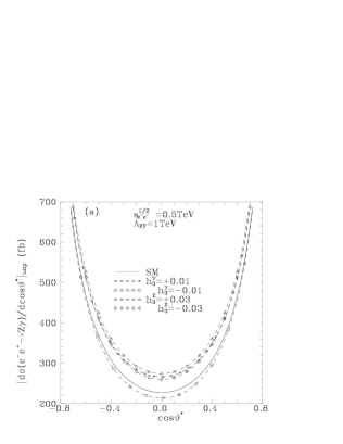
Figure 5: Standard and anomalous contributions to unpolarized $e^{-}e^{+}\to Z\gamma$ cross sections at an LC.

We present an illustration in Fig.4a,b for $ZZ$ and Fig.5a,b,c for $Z\gamma$, by choosing values for the couplings which make the SM and SM+NP curves well visible on the drawing; but of course the observability limits are found to correspond to much lower values. To be more precise, a careful study of the background should be done. One can find some preliminary studies of these effects presented at the ECFA meeting [19]. In the case of $e^{+}e^{-}\to ZZ$ there is almost no background for the $q\bar{q}l\bar{l}$ mode, but there is some background in the $q\bar{q}\nu\bar{\nu}$ mode due to the $WW$ channel. Taking them into account, a final (statistical + systematical) accuracy of the order of 1% should be expected, for a conservative integrated luminosity of $100~{}fb^{-1}$. We may even expect a better sensitivity with the higher luminosity of the TESLA design. In any case a 1% accuracy on the cross section at large angles (see Fig.4a,b), would lead to sensitivity limits for $f^{\gamma}_{4}$, $f^{Z}_{4}$, $f^{\gamma}_{5}$, $f^{Z}_{5}$ like $2.10^{-3},~{}4.10^{-3},~{}3.10^{-3},~{}7.10^{-4}$ respectively, at the one standard deviation level.

In the case of $e^{+}e^{-}\to Z\gamma$ at large angles ($|cos\theta|<0.8$) no appreciable background is expected [19]. With $100~{}fb^{-1}$, about $50000$ events should be selected, leading to an accuracy better than the 0.5% level. The sensitivity (one standard deviation) is now of $3.10^{-3}$, $5.10^{-3}$, $3.10^{-4}$, $4.10^{-4}$, $2.10^{-4}$, $4.10^{-3}$, $4.10^{-5}$, $3.10^{-4}$, for $h^{\gamma}_{1}$, $h^{Z}_{1}$, $h^{\gamma}_{2}$, $h^{Z}_{2}$, $h^{\gamma}_{3}$, $h^{Z}_{3}$, $h^{\gamma}_{4}$, $h^{Z}_{4}$, respectively. Indeed, the observability limits should be about two orders of magnitude better than the ones quoted in the LEP2 case.

Another feature of LC is the possibility of having longitudinally polarized $e^{\pm}$ beams; (a polarized $e^{-}$ beam would be in fact sufficient, like at SLC). We have therefore looked at the effect of the anomalous couplings on the $A_{LR}$ asymmetry whose expression is given in Appendix B. Note, from the expression of the SM amplitudes given in Appendix A, that the SM values of $A_{LR}$ are independent of the scattering angle and energy, taking the values

$$A_{LR}^{SM}(e^{-}e^{+}\to ZZ) = {(g^{Z}_{-})^{4}-(g^{Z}_{+})^{4}\over(g^{Z}_{-})^{4}+(g^{Z}_{+})^{4}}\simeq 0.28~{}~{},$$ (17)

$$A_{LR}^{SM}(e^{+}e^{-}\to Z\gamma) = {(g^{Z}_{-})^{2}-(g^{Z}_{+})^{2}\over(g^{Z}_{-})^{2}+(g^{Z}_{+})^{2}}\simeq 0.14~{}~{}.$$ (18)

NP departures from there relations arise very differently for the anomalous photon- and $Z$-couplings; especially in the CP-conserving case which interferes with SM. Thus, one observes a large sensitivity to the sign of certain anomalous CP conserving couplings. See Fig.6a,b for $ZZ$ and Fig.7a,b,c for $Z\gamma$. It appears therefore, that measurements of $A_{LR}$ should be very useful for disentangling the anomalous photon and Z couplings.

Application to $ZZ$ and $Z\gamma$ production at hadron colliders.
Finally we have made an illustration for $ZZ$ and $Z\gamma$ at the TEVATRON (2TeV) and at LHC (14TeV). We have chosen to illustrate the transverse momentum ($p_{T}$) distribution of one Z (both in the $ZZ$ and in the $Z\gamma$ case), as it is the one which is mostly used in the literature [18]. But we have also checked that the $ZZ$ or $Z\gamma$ invariant mass ($\sqrt{\hat{s}}$) distribution shows roughly the same features and gives the same sensitivity to the anomalous couplings. These distributions reflect the fact that CP-conserving amplitudes interfere with the SM ones, whereas the CP-violating ones always do not, as we can see in Fig.8 for the TEVATRON and Fig.9 for the LHC .

These interference patterns are somewhat less pronounced than in the illustrations for $e^{-}e^{+}$ collisions. This is due to the fact that the $p_{T}$ distributions that we are showing, are the results of integrations over regions of phase space where the quadratic term is important and partly washes out the interference term. In order to recover the same features as in the $e^{-}e^{+}$ illustrations, one should make severe cuts selecting a restricted domain in invariant mass and preferably large values of the cm scattering angle. In such a domain one can find values of the CP-conserving couplings producing a visible effect dominated by the linear (interfering) term. Such a study, which should be carefully done taking into account all the event selection criteria, is beyond the scope of this paper, but we think that it should be tried. For this purpose we have given in Appendix B the expression of the differential cross section with respect to invariant mass and c.m. scattering angle.

As far as the comparison of the sensitivities at hadron colliders and at $e^{-}e^{+}$ colliders is concerned, we would like to come back to the discussion we gave at the begining of this Section about the use of form factors, by adding a few (more or less obvious) remarks. This use of form factors is commonly done when analyzing transverse momentum or invariant mass distributions at hadron colliders, in order to take into account the fact that any given non vanishing value of an anomalous coupling, will eventually violate unitarity at sufficiently higher energies. In spite of its apparent necessity, this procedure forbids to do any clear comparison of observability limits among different colliders because they involve an integration over a large range of invariant mass $\sqrt{\hat{s}}$. We would therefore prefer another procedure that would consist in giving observability limits for the considered basic couplings (without any form factor), in restricted domains (bins) of the subprocess invariant mass. At the same collider, one could then establish a set of different observability limits, by taking a set of such domains of invariant masses in which there are enough events to analyze. This set of observability limits could then be compared among each other and also with observability limits obtained separately at different colliders and different energies.

This is an additional motivation for our suggestion to make analyses in restricted domains of invariant masses, that we already mentioned above.

4 Final discussion

In this paper we have examined the existing phenomenological description of the anomalous neutral 3-boson couplings ($\gamma\gamma Z,~{}\gamma ZZ,~{}ZZZ$), and we have reviewed the basic assumptions which allow to constrain the number and structure of the relavant couplings.

A first observation was that in the set of couplings which were commonly used for studying $Z\gamma$ production, a factor ”i” was missing making the Effective Lagrangian antihermitian. As a result, the interference patterns of the CP-conserving and the CP-violating NP amplitudes, with the SM ones, were reversed. Nevertheless, this observation does not seem to invalidate most of the presently existing experimental observability limits, since they are so low, that they are mainly arising from the quadratic part of the NP contribution. But of course, as the accuracy of the measurements is increasing, it would eventually lead to non-intuitive results.

We have therefore carefully rederived the Standard Model (SM) and the anomalous (NP) amplitudes, in order to clearly fix all conventions and normalizations. We have illustrated the corresponding effects that the various anomalous couplings induce on $ZZ$ and $Z\gamma$ production at $e^{-}e^{+}$ and hadron colliders. We have made applications for LEP2, for an LC of 500 GeV, and for the TEVATRON and the LHC. On the angular distribution, we have shown the interference patterns produced by the CP-conserving couplings and the additive contributions given by the CP-violating couplings.

In the case of LC, we have emphasized the possible role of longitudinal polarization for disentangling different sets of couplings, as in some cases the interference pattern in the $A_{LR}$ asymmetry is much more pronounced than on the unpolarized cross section.

As far as hadron colliders are concerned, we have suggested to try to make analyses in different restricted domains (bins) of invariant $ZZ$ or $Z\gamma$ masses, with large values of the c.m. scattering angle. In such a case, the inteference patterns should be comparable to the ones observable in $e^{-}e^{+}$ collisions, and much more pronounced than in a (fully integrated) transverse momentum distribution. Of course such an analysis was not possible in the $1.8~{}TeV$ TEVATRON; but it may be possible, due to the much larger expected statistics, at the upgraded TEVATRON and the LHC.

This procedure would also allow to get rid of the multiplicative form factor introduced in many previous analyses. The comparison of the various observability limits obtained at different $e^{-}e^{+}$ or hadron colliders, each one being defined for a given invariant mass range, would then be straightforward.

We have also mentioned that if we use e.g. the linear scalar sector representation appropriate for a relatively light higgs particle, then at the level of all possible $SU(2)\times U(1)$ gauge invariant $dim=6$ operators, which predict a certain pattern of anomalous $\gamma WW$ and $ZWW$ couplings, no neutral gauge boson couplings are expected. Thus if such couplings are discovered, it may mean either that for some reasons certain $dim=8$ or 10 operators are more important than those of $dim=6$; or that NP scale is nearby, thus invalidating the dimensional ordering of the $SU(2)\times U(1)$ gauge invariant operators.

We have made a specific application taking as NP effect the one due to the contributions of heavy fermions at one loop. We have discussed two cases, one in which only one set of heavy fermions is lighter than all others, and one in which the complete family is nearly degenerate. In both cases one observes that only the $f^{V}_{5}$ and $h^{V}_{3}$ couplings are generated (together with the anapole $ZWW$, $\gamma WW$ couplings in the charged sector), the other couplings requiring higher order effects. In addition, we have noticed remarkable relations among these couplings. An important difference between these two aforementioned cases is that, in the first one, the couplings behave like $1/\Lambda^{2}_{NP}$, whereas in the second they go like $1/\Lambda^{4}_{NP}$, leading to much poorer bounds on the NP scale. We should also state that, within this type of models, in order to generate observable couplings at present colliders, the NP dynamics must include a strong enhancement effect that would compensate the one loop $\alpha/4\pi$ factor. Otherwise one could expect such virtual effects to be observable only at a very high luminosity LC. In any case this example has shown how experimental constraints established on each coupling could give some indications on the NP properties.

Acknowledgments: It is a pleasure to thank Robert Sekulin for very informative discussions and suggestions.

Appendix A: The Standard Model helicity amplitudes for $f\bar{f}\to ZZ$ and $f\bar{f}\to Z\gamma$.

The invariant helicity amplitudes for the production processes of the neutral vector bosons $V_{1},V_{2}$,

$$f(k_{1},\lambda_{1})\bar{f}(k_{2},\lambda_{2})\to V_{1}(q_{1},\tau_{1})V_{2}(q_{2},\tau_{2})~{}~{},$$ (A.1)

are denoted as $F_{\lambda_{1}\lambda_{2}\tau_{1}\tau_{2}}$, where the momenta and helicities of the incoming fermions ($f,\bar{f}$) and the outgoing neutral vector bosons are indicated in parentheses in (A.1). Since at Collider energies the mass $m_{f}$ of the incoming fermion can be neglected in all cases, the dependence of the amplitude on the initial helicities is only through the combination $\lambda\equiv\lambda_{1}-\lambda_{2}$, so that the notation $F^{\lambda}_{\tau_{1}\tau_{2}}$ will be used below. Thus, there two possible values for $\lambda$ are $\lambda=-1(+1)$, corresponding to an $f_{L(R)}$ fermion interacting with a $\bar{f}_{R(L)}$ antifermion respectively; so that the $Z$ and photon couplings in (A.3,A.4) may be written as $g^{Z}_{\lambda}$ and $g^{\gamma}_{\lambda}$ respectively, as defined by the Standard Model interaction Lagrangian involving a fermion $f$ of charge $Q_{f}$ and third isospin component $t_{f}^{(3)}$,

$${\cal L}=-eV^{\mu}\bar{f}\left(g^{V}_{L}\gamma_{\mu}\frac{(1-\gamma_{5})}{2}~{}+~{}g^{V}_{R}\gamma_{\mu}\frac{(1+\gamma_{5})}{2}\right)f~{}~{},$$ (A.2)

with

$$g^{\gamma}_{L}=g^{\gamma}_{R}=Q_{f}~{}~{}~{},$$ (A.3)

$$g^{Z}_{L}=\frac{1}{s_{W}c_{W}}(t_{f}^{(3)}-Q_{f}s^{2}_{W})~{}~{}~{},~{}~{}~{}g^{Z}_{R}=\frac{1}{s_{W}c_{W}}(-Q_{f}s^{2}_{W})$$ (A.4)

For $ZZ$ production, CPT invariance implies at tree level

$$F^{\lambda}_{\tau_{1},\tau_{2}}(f\bar{f}\to ZZ)=F^{\lambda*}_{-\tau_{2},-\tau_{1}}(f\bar{f}\to ZZ)~{}~{},$$ (A.5)

while CP invariance would demand

$$F^{\lambda}_{\tau_{1},\tau_{2}}(f\bar{f}\to ZZ)=F^{\lambda}_{-\tau_{2},-\tau_{1}}(f\bar{f}\to ZZ)~{}~{},$$ (A.6)

even at higher orders. Since the Standard Model amplitudes for $f\bar{f}\to ZZ$ satisfy CP invariance, the tree level standard helicity amplitudes are real and may be written, following the notations of [2], as

$$F^{\lambda}_{\tau_{1}\tau_{2}}(f\bar{f}\to ZZ~{};~{}SM)=-e^{2}(g^{Z}_{\lambda})^{2}~{}\frac{A^{\lambda Z}_{\tau_{1}\tau_{2}}}{4\beta^{2}\sin^{2}\vartheta^{*}+\gamma^{-4}}~{}~{},$$ (A.7)

where

$$A^{\lambda Z}_{\tau_{1},\tau_{2}}=2\sin\vartheta^{*}\left[2\lambda\cos\vartheta^{*}(\beta^{2}-\tau_{1}\tau_{2})-(1+\beta^{2})(\tau_{2}-\tau_{1})\right]~{}\mbox{for}~{}\tau_{1}\tau_{2}\neq 0~{},$$ (A.8)

$$A^{\lambda Z}_{0,\tau}=A^{\lambda Z}_{-\tau,0}=\frac{2\sqrt{2}}{\gamma}(1-\lambda\tau\cos\vartheta^{*})[\lambda\tau(1+\beta^{2})+2\cos\vartheta^{*}]~{}\mbox{for}~{}\tau\neq 0~{},$$ (A.9)

$$A^{\lambda Z}_{00}=-~{}\frac{4\lambda\sin(2\vartheta^{*})}{\gamma^{2}}~{}~{},$$ (A.10)

and $\vartheta^{*}$ is the c.m. $Z$ scattering angle with respect to the $f$-beam axis, while

$$\beta=\sqrt{1-~{}\frac{4m_{Z}^{2}}{\hat{s}}}~{}~{}~{},~{}~{}~{}\gamma=\frac{1}{\sqrt{1-\beta^{2}}}~{}.$$ (A.11)

Notice that (A.7-A.10) define also our conventions on the relative fermion and antifermion phases.

Correspondingly the SM helicity amplitudes for $f\bar{f}\to Z\gamma$ are

$$F^{\lambda}_{\tau_{1}\tau_{2}}(f\bar{f}\to Z\gamma~{};~{}SM)=-e^{2}g^{Z}_{\lambda}g^{\gamma}_{\lambda}~{}\frac{\hat{s}}{\hat{s}-m_{Z}^{2}}~{}A^{\lambda\gamma}_{\tau_{1}\tau_{2}}~{}~{},$$ (A.12)

where

$$A^{\lambda\gamma}_{\tau_{1},\tau_{2}} = -~{}\frac{1}{\sin\vartheta^{*}}\Big{\{}\tau_{2}-\tau_{1}+\lambda\cos\vartheta^{*}(-1+\tau_{1}\tau_{2})$$ (A.13)

$$+~{}\frac{m_{Z}^{2}}{\hat{s}}[\tau_{1}+\tau_{2}+\lambda(1+\tau_{1}\tau_{2})\cos\vartheta^{*}]\Big{\}}~{},$$

$$A^{\lambda\gamma}_{0,\tau_{2}} = 2\sqrt{2}\lambda\tau_{2}~{}\frac{m_{Z}}{\sqrt{\hat{s}}}~{}.$$ (A.14)

Appendix B: Cross section for LEP, LC and the Hadron Colliders.

The full helicity amplitudes for $V_{1}V_{2}$ ($V_{1}=Z,~{}V_{2}=Z,\gamma$) production through the process (A.1) are obtained by adding the SM contributions in (A.7, A.12) and the NP ones appearing in (7, 8, 9) as

$$F^{\lambda}_{\tau_{1}\tau_{2}}(f\bar{f}\to V_{1}V_{2})=F^{\lambda}_{\tau_{1}\tau_{2}}(f\bar{f}\to V_{1}V_{2}~{};~{}SM)+F^{\lambda}_{\tau_{1}\tau_{2}}(f\bar{f}\to V_{1}V_{2}~{};~{}NP)~{},$$ (B.1)

and they are normalized so that the unpolarized differential cross sections are given by

$$\frac{d\hat{\sigma}(f\bar{f}\to ZZ)}{d\cos\vartheta^{*}} = \frac{\hat{s}}{2}\left(1-~{}\frac{4m_{Z}^{2}}{\hat{s}}\right)^{{1\over 2}}~{}\frac{d\hat{\sigma}(f\bar{f}\to ZZ)}{d\hat{t}}$$ (B.2)

$$=\frac{1}{128\pi\hat{s}}\left(1-~{}\frac{4m_{Z}^{2}}{\hat{s}}\right)^{{1\over 2}}\sum_{\tau_{1}\tau_{2}}\left[|F^{\lambda=1}_{\tau_{1}\tau_{2}}|^{2}+|F^{\lambda=-1}_{\tau_{1}\tau_{2}}|^{2}\right]~{},$$

$$\frac{d\hat{\sigma}(f\bar{f}\to Z\gamma)}{d\cos\vartheta^{*}} = \frac{(\hat{s}-m_{Z}^{2})}{2}~{}\frac{d\hat{\sigma}(f\bar{f}\to Z\gamma)}{d\hat{t}}$$ (B.3)

$$=\frac{(\hat{s}-m_{Z}^{2})}{128\pi\hat{s}^{2}}\sum_{\tau_{1}\tau_{2}}\left[|F^{\lambda=1}_{\tau_{1}\tau_{2}}|^{2}+|F^{\lambda=-1}_{\tau_{1}\tau_{2}}|^{2}\right]~{}.$$

Note that in (B.2), the identity of the two final $Z$ is taken into account by imposing the constrain $0\leq\cos\vartheta^{*}\leq 1$.

The Left-Right asymmetry measurable at an LC is defined by

$$A_{LR}(e^{-}e^{+}\to V_{1}V_{2}) = [\frac{d\hat{\sigma}(e_{L}^{-}e_{R}^{+}\to V_{1}V_{2})}{d\cos\vartheta^{*}}-\frac{d\hat{\sigma}(e_{R}^{-}e_{L}^{+}\to V_{1}V_{2})}{d\cos\vartheta^{*}}]\times$$ (B.4)

$$[\frac{d\hat{\sigma}(e_{L}^{-}e_{R}^{+}\to V_{1}V_{2})}{d\cos\vartheta^{*}}+\frac{d\hat{\sigma}(e_{R}^{-}e_{L}^{+}\to V_{1}V_{2})}{d\cos\vartheta^{*}}]^{-1}$$

$$= \frac{\sum_{\tau_{1}\tau_{2}}\left[|F^{\lambda=1}_{\tau_{1}\tau_{2}}|^{2}-|F^{\lambda=-1}_{\tau_{1}\tau_{2}}|^{2}\right]}{\sum_{\tau_{1}\tau_{2}}\left[|F^{\lambda=1}_{\tau_{1}\tau_{2}}|^{2}+|F^{\lambda=-1}_{\tau_{1}\tau_{2}}|^{2}\right]}$$

Finally the $p_{T}$ distribution at a hadron collider, with c.m. energy $\sqrt{s}$, is determined by

$$\frac{d\sigma(H_{1}H_{2}\to V_{1}V_{2}+...)}{dp_{T}^{2}dy_{1}dy_{2}}=\tau\Sigma^{V_{1}V_{2}}(x_{a},x_{b})~{}~{},$$ (B.5)

where

$$\Sigma^{ZZ}(x_{a},x_{b})=\sum_{j}\left[q_{j}(x_{a})\bar{q}_{j}(x_{b})+\bar{q}_{j}(x_{a})q_{j}(x_{b})\right]\frac{d\hat{\sigma}(q\bar{q}\to ZZ)}{d\hat{t}}~{},$$ (B.6)

$$\Sigma^{Z\gamma}(x_{a},x_{b})=\sum_{j}\left[q_{j}(x_{a})\bar{q}_{j}(x_{b})+\bar{q}_{j}(x_{a})q_{j}(x_{b})\right]\frac{d\hat{\sigma}(q\bar{q}\to Z\gamma)}{d\hat{t}}~{},$$ (B.7)

The summation extend over all quark and antiquarks inside the hadrons $H_{1},~{}H_{2}$. Note that the distributions considered in this paper are symmetrical in $\hat{t}$, $\hat{u}$ interchange. $\tau=\hat{s}/s$, while $(x_{a},x_{b})$ are fully determined in terms of the rapidities ($y_{1},~{}y_{2}$) and the (opposite) transverse momenta of the two final gauge bosons:

$$x_{a}={1\over 2}[x_{1T}e^{y_{1}}+x_{2T}e^{y_{2}}]\ \ \ \ \ \ x_{b}={1\over 2}[x_{1T}e^{-y_{1}}+x_{2T}e^{-y_{2}}]$$ (B.8)

where $x_{iT}={2\over\sqrt{s}}~{}(p^{2}_{T}+m^{2}_{V_{i}})^{{1\over 2}}$. In the integration over $y_{1}$ and $y_{2}$ we impose a cut at $|y_{i}|<2$.

We will also discuss the invariant mass and c.m. scattering angle distributions given by

$$\frac{d\sigma(H_{1}H_{2}\to V_{1}V_{2}+...)}{d\hat{s}d\cos\vartheta^{*}d\bar{y}}=J\tau\Sigma^{V_{1}V_{2}}(x_{a},x_{b})~{}~{},$$ (B.9)

where $J(Z\gamma)={\hat{s}-m^{2}_{Z}\over 2\hat{s}}$, $J(ZZ)={1\over 2}\sqrt{1-{4m^{2}_{Z}\over\hat{s}}}$. $\bar{y}$ is the boost defined as $\bar{y}=y_{1}-y^{*}_{1}=y_{2}-y^{*}_{2}$, with $thy^{*}_{1}=\beta_{1}^{*}\cos\vartheta^{*}$, $thy^{*}_{2}=-\beta_{2}^{*}\cos\vartheta^{*}$ and $\beta^{*}_{1}={\hat{s}-m^{2}_{Z}\over\hat{s}^{+}m^{2}_{Z}}$, $\beta^{*}_{2}=1$ for $Z\gamma$, but $\beta^{*}_{1}=\beta^{*}_{2}=\sqrt{1-{4m^{2}_{Z}\over\hat{s}}}$ for $ZZ$. With these variables, $x_{a}=e^{\bar{y}}\sqrt{\tau}$, $x_{b}=e^{-\bar{y}}\sqrt{\tau}$.

Figure 1: Feynman rule for the general $V_{1}V_{2}V_{3}$ vertex.

     

Figure 2: Standard and anomalous contributions to the unpolarized $e^{-}e^{+}\to ZZ$ cross section at LEP.

     

Figure 3: Standard and anomalous contributions to the unpolarized $e^{-}e^{+}\to Z\gamma$ cross sections at LEP.

     

Figure 4: Standard and anomalous contributions to unpolarized $e^{-}e^{+}\to ZZ$ cross sections at an LC.

     

     

Figure 6: Standard and anomalous contributions to Left-Right asymmetries in the $e^{-}e^{+}\to ZZ$ cross sections at an LC.

     

Figure 7: Standard and anomalous contributions to Left-Right asymmetries in the $e^{-}e^{+}\to Z\gamma$ cross sections at an LC.

     

     

Figure 8: Standard and anomalous contributions to the $pp\to ZZ~{},~{}Z\gamma$ inclusive cross sections at the Tevatron.

     

     

Figure 9: Standard and anomalous contributions to the $pp\to ZZ~{},~{}Z\gamma$ inclusive cross sections at LHC.

References

- [1] K.J.F. Gaemers and G.J. Gounaris, Z. f. Phys. (1979) 259.
- [2] K. Hagiwara, R.D. Peccei and D. Zeppenfeld, Nucl. Phys. (1987) 253.
- [3] H. Georgi, Nucl. Phys. (1991) 339.
- [4] G.J. Gounaris and F.M. Renard, Z. f. Phys. (1993) 133.
- [5] W. Buchmüller, D. Wyler, Nucl. Phys. (1986) 621.
- [6] J.Wudka, Int. J. Mod. Phys. A9(1994)(2301); J. Ellison and J. Wudka, Ann. Rev. Nucl. Sci. 48 (1998) 48.
- [7] H. Aihara et. al., Summary of the Working Subgroup on Anomalous Gauge Boson Interactions of the DPF Long-Range Planning Study, to be published in “Electroweak Symmetry Breaking and Beyond the Standard Model”, Editors T. Barklow, S. Dawson, H. Haber and J. Siegrist, LBL-37155, hep-ph/9503425; Report of the ‘Triple Gauge Boson Couplings’ Working Group, G.J.Gounaris, J-L.Kneur and D.Zeppenfeld (convenors), in Physics at LEP2, eds. G.Altarelli, T.Sjöstrand and F.Zwirner, CERN Report 96-01 (1996).
- [8] K. Hagiwara, S. Ishhara, R. Szalapski and D. Zeppenfeld Phys. Rev. (1993) 2182; G.J. Gounaris and C.G. Papadopoulos Eur. Phys. J. (1998) 365.
- [9] T. Appelquist and C. Bernard, Phys. Rev. (1980) 200; T.Appelquist and Guo-Hong Wu, Phys. Rev. (1993) 3235; H.-J. He, Y.-P. Kuang and C.-P. Yuan, DESY-97-056. Lectures given at CCAST Workshop on Physics at TeV Energy Scale, Beijing, China, 15-26 Jul 1996;
- [10] M.Kuroda, F.M.Renard and D. Schildknecht, Phys. Lett. (1987) 366; M. Kuroda, J. Maalampi, D. Schildknecht and K. H. Schwarzer, Nucl. Phys. B284, 271 (1987); Phys. Lett. 190, 217 (1987); C. Grosse-Knetter, I. Kuss and D. Schildknecht, Phys. Lett. B358, 87 (1995)
- [11] The LEP Collaborations ALEPH, DELPHI, L3, Opal, the LEP Electroweak Working Group and the SLD Heavy Flavour and Electroweak Groups, CERN-EP/99-15.
- [12] CDF Collaboration, F. Abe et.al. Phys. Rev. Lett. (1995) 1936
- [13] D0 Collaboration, S. Abachi et.al. Phys. Rev. (1997) 6742.
- [14] G.J. Gounaris, J. Layssac and F.M. Renard, Phys. Lett. (1994) 146; G.J. Gounaris, J. Layssac, J.E. Paschalis and F.M. Renard, Z. f. Phys. (1995) 619; G.J. Gounaris, F.M. Renard and G. Tsirigoti, Phys. Lett. (1995) 212; G.Gounaris, F.M.Renard and N.D.Vlachos, Nucl.Phys. B459(1996)51.
- [15] F.M. Renard, Nucl. Phys. (1982) 93; A. Barroso, F. Boudjema, J. Cole and N. Dombey, Z. f. Phys. (1985) 149.
- [16] F. Boudjema, Proc. of the Workshop on Collisions at 500GeV: The Physics Potential, DESY 92-123B (1992) p.757, edited by P.M. Zerwas.
- [17] G.J. Gounaris, J. Layssac and F.M. Renard, ”New Physics contributions to anomalous and self-couplings”, preprint in preparation.
- [18] U. Baur, E.L. Berger, Phys. Rev. (4889) 1993; U. Baur, T Han anf J. Ohnemus, Phys. Rev. (2823) 1998 and references therein.
- [19] J. Alcaraz, report presented at the ECFA meeting, Oxford, March 1999.
- [20] L3 Collaboration, M. Acciari et.al. Phys. Lett. (281) 1999; Phys. Lett. (363) 1999.
- [21] Opportunities and Requirements for Experimentation at a Very High Energy Collider, SLAC-329(1928); Proc. Workshops on Japan Linear Collider, KEK Reports, 90-2, 91-10 and 92-16; P.M. Zerwas, DESY 93-112, Aug. 1993; Proc. of the Workshop on Collisions at 500 GeV: The Physics Potential, DESY 92-123A,B,(1992), C(1993), D(1994), E(1997) ed. P. Zerwas; E. Accomando et.al. Phys. Rep. (1) 1998.