Evolution of a global string network in a matter-dominated universe

Abstract

We evolve the network of global strings in the matter-dominated universe by means of numerical simulations. The existence of the scaling solution is confirmed as in the radiation-dominated universe but the scaling parameter $\xi$ takes a slightly smaller value, $\xi\simeq 0.6\pm 0.1$, which is defined as $\xi=\rho_{s}t^{2}/\mu$ with $\rho_{s}$ the energy density of global strings and $\mu$ the string tension per unit length. The change of $\xi$ from the radiation to the matter-dominated universe is consistent with that obtained by Albrecht and Turok by use of the one-scale model. We also study the loop distribution function and find that it can be well fitted with that predicted by the one-scale model, where the number density $n_{l}(t)$ of the loop with the length $l$ is given by $n_{l}(t)=\nu/[t^{2}(l+\kappa t)^{2}]$ with $\nu\sim 0.040$ and $\kappa\sim 0.48$. Thus, the evolution of the global string network in the matter-dominated universe can be well described by the one-scale model as in the radiation-dominated universe.

Cosmic strings are formed in a class of cosmological phase transitions [2]. Among them, gauged or local strings have been extensively studied because they could produce density fluctuations responsible for the large-scale structure formation and the cosmic microwave background anisotropy [3]. A lot of analytical and numerical studies have been done to confirm that after some relaxation period a local string network enters the scaling regime. In this regime, the large-scale behavior of a network scales with the Hubble radius and the energy density of a network is given by

$$\rho_{\rm string}=\xi\mu/t^{2}\>,$$ (1)

where $\xi$ is a constant irrespective of cosmic time. [4, 5, 6, 7]. Long strings intercommute to make loops [6, 7, 8], which decay through radiating gravitational waves [9]. But an alternative scenario was recently proposed that long strings directly emit massive particles and lose their own energy [10]. Thus, though the mechanism to drive a network to the scaling regime is still in dispute, the existence of the scaling solution is undoubted.

On the other hand, global strings have been less investigated and considered only in the context of axion cosmology [11, 12, 13, 14, 15, 16]. It was assumed without direct verification that a global string network relaxes into the scaling solution just as the local counterpart, where long strings intercommute to create loops with a typical size that is comparable with the horizon scale and loops decay through emitting Nambu-Goldstone (NG) bosons. However, since global strings have a long-range interaction their dynamics could be different from that of local strings. In fact our numerical analysis of the evolution of a complex scalar field in 2+1 dimensions revealed that the global “strings” do not relax into the scaling solution but the number of defects per horizon volume increases logarithmically with time due to the long-range interaction [17]. In the previous paper [18] we examined the evolution of a global string network in the radiation-dominated universe by numerically solving the equation of motion for a complex scalar field representing a global string. Then the above picture was confirmed. The scaling parameter $\xi$ takes a constant value and becomes $\xi\sim(0.9-1.3)$, irrespective of the cosmic time. Furthermore, one of the authors (M.Y.) [19] has found that the number density $n_{l}(t)$ of the loop with the length $l$ can be well fitted by the formula predicted from the so-called one-scale model, that is, $n_{l}(t)=\nu/[t^{3/2}(l+\kappa t)^{5/2}]$ with $\nu\sim 0.0865$ and $\kappa\sim 0.535$. Thus, the evolution of a global string network in the radiation dominated universe is well described by the one-scale model proposed by Kibble [20, 21, 22].

In this paper, for a complete understanding, we study the evolution of a global string network in the matter-dominated universe, concretely, whether it can be well described by the one-scale model as in the radiation-dominated universe and, if at all, we clarify the relation between scaling parameters in both eras.

We consider the following Lagrangian density for a complex scalar field $\Phi(x)$,

$${\cal L}[\Phi]=g_{\mu\nu}(\partial^{\mu}\Phi)(\partial^{\nu}\Phi)^{\dagger}-V_{\rm eff}[\Phi,T]\>,$$ (2)

where $g_{\mu\nu}$ is identified with the Robertson-Walker metric and the effective potential $V_{\rm eff}[\Phi,T]$ is given by

$$V_{\rm eff}[\Phi,T]=\frac{1}{2}\lambda(\Phi\Phi^{\dagger}-\eta^{2})^{2}+\frac{1}{3}\lambda T^{2}\,\Phi\Phi^{\dagger}\>,$$ (3)

which represents a typical second-order phase transition and the $U(1)$ symmetry is broken below the critical temperature $T_{c}=\sqrt{3}\eta$.

For cosmological purposes, it would be desirable to trace the evolution of strings in the transition regime from the radiation-dominated era to the matter-dominated era. Due to the limitation of our computer powers, however, we concentrate on the evolution of a global string network during the matter-domination alone in this paper. Since the scaling property is expected to be reached irrespective of initial conditions if at all, we start simulations from a symmetric state with the equations of motion given in the matter domination. Strings are formed soon and they evolve in the matter-domination. As will be shown later, we confirm the scaling behavior in the matter-dominated regime and find that $\xi$ in this era is not different from that in the radiation-domination by more than a factor of 2. Hence we expect that transition from the radiation-dominated era to the matter-dominated era does not give rise to any significant cosmological effects, justifying our approach.

In the matter-dominated universe, the equation of motion is given by

$$\ddot{\Phi}(x)+3H\dot{\Phi}(x)-\frac{1}{R(t)^{2}}\nabla^{2}\Phi(x)=-V^{\prime}_{\rm eff}[\Phi,T]\>,$$ (4)

where the prime represents the derivative $\partial/\partial\Phi^{\dagger}$ and $R(t)$ is the scale factor which grows in proportion to $t^{2/3}$. We define $\alpha(T)$ [$\alpha(T)>1$] as $\alpha(T)\equiv\rho_{\rm mat}(T)/\rho_{\rm rad}(T)$ with $\rho_{\rm mat}(T)$ being the contribution to the energy density from non-relativistic particles and $\rho_{\rm rad}(T)$ being the contribution from relativistic particles at the temperature $T$. Then,

$$\alpha(T)=\alpha_{c}(T_{c}/T)\>,$$ (5)

with $\alpha_{c}\equiv\rho_{\rm mat}(T_{c})/\rho_{\rm rad}(T_{c})$. Therefore, the Hubble parameter $H=\dot{R}(t)/R(t)$ and the cosmic time $t$ are given by

$$H^{2} = \alpha(T)\frac{8\pi}{3m_{\rm pl}^{2}}\frac{\pi^{2}}{30}g_{*}T^{4}$$ (6)

$$= \alpha_{c}\frac{4\sqrt{3}\pi^{3}\eta g_{*}}{45m_{\rm pl}^{2}}T^{3},$$ (7)

$$~{}~{}~{}~{}~{}t = \frac{2}{3H}\equiv\frac{\epsilon}{T^{3/2}}\>,$$ (8)

where $m_{\rm pl}=1.2\times 10^{19}$ GeV is the Plank mass and $g_{*}$ is the total number of degrees of freedom for the relativistic particles. We define the dimensionless parameter $\zeta$ as

$$\zeta\equiv\frac{\epsilon}{\eta^{1/2}}=\left(\frac{5m_{\rm pl}^{2}}{\sqrt{3}\alpha_{c}\pi^{3}g_{*}\eta^{2}}\right)^{1/2}\>.$$ (9)

In our simulation, we take $\zeta=8$ and $4$ to investigate $\zeta$ dependence on the result. We take the initial time $t_{i}=t_{c}/(2\sqrt{2})$ corresponding to $T_{i}=2T_{c}$ and the final time $t_{f}=70(140)\,t_{i}$, where $t_{c}$ is the epoch with $T=T_{c}$. Since the $U(1)$ symmetry is restored at the initial time $t=t_{i}$, we adopt as the initial condition the thermal equilibrium state with the mass squared,

$$m^{2}=\left.\frac{d^{2}V_{\rm eff}[|\Phi|,T]}{d|\Phi|^{2}}\right|_{|\Phi|=0}\>,$$ (10)

which is the inverse curvature squared of the potential at the origin at $t=t_{i}$.

Below we measure all of the physical quantities in units of $t_{i}$. Then the equation of motion is given by

$$\ddot{\Phi}(x)+\frac{2}{t}\dot{\Phi}(x)-\frac{1}{t^{4/3}}\nabla^{2}\Phi(x)=-\left(|\Phi|^{2}+\frac{\zeta^{2}}{6\sqrt{3}\,t^{4/3}}-\frac{\zeta^{2}}{24\sqrt{3}}\right)\Phi^{\dagger}\>,$$ (11)

where $\lambda$ is set to unity for brevity. The scale factor $R(t)$ is normalized as $R(1)=1$.

Using the second-order leap-frog method (see Ref. [19] for details), we evolve the global string networks in the matter-dominated universe. In order to judge whether the global string network relaxes into the scaling regime in the matter-dominated universe, we give time development of the scaling parameter $\xi$ defined as $\rho=\xi\mu/t^{2}$. In our simulations, a lattice is identified with a part of a string core if the potential energy density there is larger than that corresponding to the field value of a static cylindrically-symmetric solution at $r=\delta x_{\rm{phys}}/\sqrt{2}$.

We perform the simulations in seven different sets of lattice sizes, spacings, and $\zeta$ (see Table I, II). In cases (1) and (5), the box size is nearly equal to the horizon volume $(H^{-1})^{3}$ and the lattice spacing to a typical width $\delta\sim 1.0/(\sqrt{2}\eta)$ of a string at the final time $t_{f}$. For each case, we simulate the system from 10 (Eqs. (1)-(6)) or 300 (Eq. (7)) different thermal initial conditions.

If the simulation box is much larger than the horizon volume, it is reasonable to think that the boundary effect is negligible. But, in our simulation, the simulation box is comparable with or at most $4^{3}$ times as large as the horizon volume at the final time of the simulation so that we should be careful to avoid possible boundary effects. In fact, a long-range force works between global strings so that the boundary effect cannot necessarily be neglected if the number of long strings in the simulation box is very small. As shown later, there are only a few long strings in our case so that the boundary effect could be significant. Hence in this paper we run simulations with two different boundary conditions of distinct features and employ a large enough simulation box so that the results with the different boundary conditions converge to each other. We thereby obtain a result free from the boundary effects.

First, we adopt the periodic boundary condition, under which a string feels an attractive force from the boundary and there exists no infinite string so that strings can completely disappear in the simulation box if the Hubble radius becomes larger than the dimension of the simulation box. Figure 1 represents time development of $\xi$ with $\zeta=8$ (cases(1),(3),(4)) under this boundary condition. In case (1) with the smallest box, the boundary effect is so significant that strings tend to disappear, which is inconsistent with the result in Refs. [20, 21, 22]. The larger the box size is, the less important the boundary effect is. In case (3) corresponding to the largest box simulations, the boundary effect is less significant so that $\xi$ seems to relax to a constant with $\xi\sim 0.49\pm 0.02$.

TABLE I.: Three different sets of the simulations under the periodic boundary condition.

Case	Lattice	Lattice spacing	$\zeta$	Realization	${\rm Box~{}size}/H^{-1}$	$\xi$
	number	[unit = $t_{i}R(t)$]			(at final time)
(1)	$128^{3}$	$\sqrt[3]{70}/85$	8	10	1(at 70)	Disappearance
(3)	$256^{3}$	$\sqrt[3]{70}/85$	8	10	2(at 70)	$0.50\pm 0.02$
(4)	$256^{3}$	$2\sqrt[3]{70}/85$	8	10	4(at 70)	$0.49\pm 0.02$

TABLE II.: Seven different sets of the simulations under the reflective boundary condition.

Case	Lattice	Lattice spacing	$\zeta$	Realization	${\rm Box~{}size}/H^{-1}$	$\xi$
	number	[unit = $t_{i}R(t)$]			(at final time)
(1)	$128^{3}$	$\sqrt[3]{70}/85$	8	10	1(at 70)	$1.93\pm 0.04$
(2)	$128^{3}$	$2\sqrt[3]{70}/85$	8	10	2(at 70)	$1.03\pm 0.03$
(3)	$256^{3}$	$\sqrt[3]{70}/85$	8	10	2(at 70)	$1.13\pm 0.02$
(4)	$256^{3}$	$2\sqrt[3]{70}/85$	8	10	4(at 70)	$0.72\pm 0.03$
(5)	$128^{3}$	$\sqrt[3]{140}/85$	4	10	1(at 140)	$1.36\pm 0.06$
(6)	$256^{3}$	$\sqrt[3]{140}/85$	4	10	2(at 140)	$1.21\pm 0.02$
(7)	$128^{3}$	$2\sqrt[3]{70}/85$	4	300	2(at 70)	$1.25\pm 0.02$

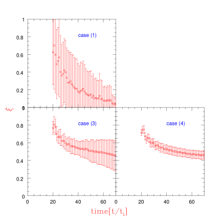
FIG. 1.: Time development of $\xi$ under the periodic boundary condition. Symbols ($\Box$) represent time development of $\xi$. The vertical lines denote a standard deviation.

Next we adopt the reflective boundary condition, where $\nabla^{2}\Phi(x)$ on the boundary points disappears. Under this boundary condition, a string suffers a repulsive force from the boundary so that a string near the boundary intercommutes less often than that near the center of the simulation box because the partner to intercommute only lies in the inner direction of the boundary. Thus, the number of the strings tends to be more than that in the real universe. Figures 2 and 3 represent time development of $\xi$ with $\zeta=8$ [cases(1)-(4)] and $\zeta=4$ [cases(5)-(7)], where $\xi$ becomes a constant irrespective of time with (1) $1.93\pm 0.04$, (2) $1.03\pm 0.03$, (3) $1.13\pm 0.02$, (4) $0.72\pm 0.03$, (5) $1.36\pm 0.06$, (6) $1.21\pm 0.04$, and (7) $0.72\pm 0.03$. $\xi$ has larger values in smaller-box simulations due to the boundary effect as explained above. Also, for larger-box simulations, $\xi$ depends very little on $\zeta$.

From the results of the largest-box simulations containing the largest number of the Hubble volume at the final epoch, we conclude that $\xi$ converges to a constant $\xi\simeq 0.6\pm 0.1$ irrespective of the boundary conditions. This result will be supported later by comparing it with our previous results in the radiation-dominated regime [18, 19] through an analytic model of Albrecht and Turok [4].

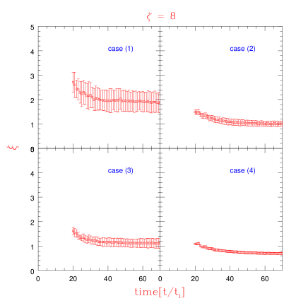
FIG. 2.: Time development of $\xi$ in the cases from (1) to (4) with $\zeta=8$ under the reflective boundary condition. Symbols ($\Box$) represent time development of $\xi$. The vertical lines denote a standard deviation over different initial conditions.

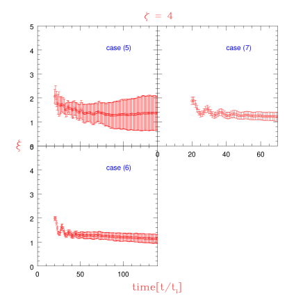
FIG. 3.: Time development of $\xi$ in the cases from (5) to (7) with $\zeta=4$ under the reflective boundary condition.

Next we investigate the loop distribution, which is predicted by Kibble’s one-scale model [20, 21, 22] as

$$n_{l}(t)=\nu/[t^{2}(l+\kappa t)^{2}]\>,$$ (12)

where $\nu$ is a constant, $l$ is the length of a loop, and the logarithmic dependence of $\mu$ is neglected. In contrast with local strings, the dominant energy loss mechanism of global strings is the radiation of the associated Nambu-Goldstone field [11]. We define the radiation power $P$ as $P=\kappa\mu$ where $\kappa$ is a constant.

We determine whether the loop distribution in the simulation coincides with the above function. Since case (4) with the largest box takes too much time for one realization, we investigate the loop distribution for case (7) under the reflective boundary condition. The loop distribution is depicted in Fig. 4 in case (7) at $t=40,50,60,$ and 70. Since long strings are rare, we cut the length of loops into bins with the width 5$\times\delta x$. Then, we divide 300 realizations into 6 groups comprised of 50 realizations and we summed the number of loops over 50 realizations for each groups. The dot represents the number of loops averaged over six groups and the dashed line represents the standard deviation. They can be simultaneously fitted with the above formula if one takes $\nu\sim 0.040$ and $\kappa\sim 0.48$. Fittings for $\kappa$ and $\nu$ are also given in Fig. 5. Thus, the loop production function as well as the large scale behavior of the string scales together for the global string network. Note that $\kappa$ takes almost the same value both in the matter- and radiation-dominated universe, which implies that NG bosons emission is not affected by the background universe and the large-scale behavior of a string network but is decided by the fundamental physics near a string segment.

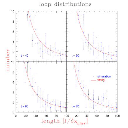
FIG. 4.: Loop distributions at $t=40,50,60,70$ are depicted. The number is summed over the box size [$128(\delta x)^{3}$] and 50 realizations for each groups. Bins are cut every 5$\times\delta x$.

FIG. 5.: Fittings for $\kappa$ and $\nu$. The cross point represents the best fit values for $\kappa$ and $\nu$. The solid circle denotes $68\%$ C.L.

As discussed in [4], the one-scale model can predict the scaling parameter $\xi_{m}$ in the matter domination from $\xi_{r}$ in the radiation domination. From the Nambu-Goto action together with the intercommutation effect, the evolution of the string energy density $\rho$ in the expanding universe is given by

$$d\rho/dt = -3H\rho+(1-2V^{2})H\rho-c\rho/L,$$ (13)

$$= -3H\rho+H^{2}L\rho-c\rho/L,$$ (14)

where $L=t/\sqrt{\xi}$ is the characteristic scale with $\rho=\mu/L^{2}$, $V^{2}$ is the average velocity squared of a string, and $c$ is a constant representing the intercommutation efficiency. Defining $\gamma$ as $\gamma=H^{-1}/L$, the evolution of $\gamma$ is given by

$$\frac{d\gamma}{dt}=-\frac{H}{2}\left\{c\gamma^{2}-[2\,\dot{(H^{-1})}-3]\gamma-1\right\}.$$ (15)

Then, in the radiation-domination with $\dot{(H^{-1})}=2$, we obtain the fixed point $\gamma_{r}$ given by

$$\gamma_{r}=(1+\sqrt{1+4c})/2c.$$ (16)

On the other hand, in the matter domination with $\dot{(H^{-1})}=3/2$, we obtain the fixed point $\gamma_{m}$ given by

$$\gamma_{m}=1/\sqrt{c}.$$ (17)

Considering $\xi_{r}=\gamma_{r}^{2}/4$ and $\xi_{m}=4\gamma_{m}^{2}/9$, we find the relation between $\xi_{r}$ and $\xi_{m}$,

$$\xi_{m}=\frac{16}{9}\frac{\xi_{r}}{(2\sqrt{\xi_{r}}+1)}.$$ (18)

Putting $\xi_{r}\sim(0.9-1.3)$ [19] into the relation, $\xi_{m}$ is predicted to be $0.6-0.7$, which coincides with our numerical results.

In this paper, we investigated the evolution of a global string network in the matter-dominated universe. The network relaxes into the scaling regime as in the radiation-dominated universe but the scaling parameter $\xi_{m}$ takes a smaller value, $\xi_{m}\simeq 0.6\pm 0.1$, which is consistent with the value predicted from $\xi_{r}$ by use of the formula obtained by Albrecht and Turok [4]. The loop distribution is also obtained and compared with that predicted by the one-scale model, where the number density $n_{l}(t)$ of the loop with the length $l$ is given by $n_{l}(t)=\nu/(t^{2}[l+\kappa t)^{2}]$. With $\nu\simeq 0.040$ and $\kappa\simeq 0.48$, the loop distribution function can be well fitted with that predicted by the one-scale model. Thus, the evolution of the global string network in the matter-dominated universe can be well described by the one-scale model as in the radiation-dominated universe.

This work was partially supported by the Japanese Grant-in-Aid for Scientific Research from the Monbusho, Nos. 10-04558 (M.Y.), 11740146 (J.Y.), and “Priority Area: Supersymmetry and Unified Theory of Elementary Particles (# 707)” (J.Y. and M.K.).

REFERENCES

- [1]
- [2] T. W. B. Kibble, J. Phys. A 9, 1387 (1976).
- [3] For a review, A. Vilenkin and E. P. S. Shellard, Cosmic String and Other Topological Defects (Cambridge University Press, Cambridge, England, 1994).
- [4] A. Albrecht and N. Turok, Phys. Rev. D 40, 973 (1989).
- [5] A. Albrecht and N. Turok, Phys. Rev. Lett. 54, 1868 (1985).
- [6] D. P. Bennett and F. R. Bouchet, Phys. Rev. Lett. 60, 257 (1988); 63, 2776 (1989); Phys. Rev. D 41, 2408 (1990).
- [7] B. Allen and E. P. S. Shellard, Phys. Rev. Lett. 64, 119 (1990).
- [8] D. Austin, E. J. Copeland, and T. W. B. Kibble, Phys. Rev. D 48, 5594 (1993); E. Copeland, T. W. B. Kibble, and D. Austin, ibid. 45, 1000 (1992).
- [9] A. Vilenkin, Phys. Rev. Lett. 46, 1169 (1981); 46, 1496(E) (1981).
- [10] G. R. Vincent, M. Hindmarsh, and M. Sakellariadou, Phys. Rev. D 56, 637 (1997); G. R. Vincent, N. D. Antunes, and M. Hindmarsh, Phys. Rev. Lett. 80, 2277 (1998).
- [11] R. L. Davis, Phys. Rev. D 32, 3172 (1985).
- [12] R. L. Davis, Phys. Lett. 180B, 225 (1986); R. L. Davis and E. P. S. Shellard, Nucl. Phys. B324, 167 (1989).
- [13] D. Harari and P. Sikivie, Phys. Lett. B 195, 361 (1987); C. Hagmann and P. Sikivie, Nucl. Phys. B363, 247 (1991).
- [14] A. Dabholkar and J. M. Quashnock, Nucl. Phys. B333, 815 (1990).
- [15] R. A. Battye and E. P. S. Shellard, Nucl. Phys. B423, 260 (1994); Phys. Rev. Lett. 73, 2954 (1994).
- [16] R. A. Battye and E. P. S. Shellard, Phys. Rev. D 53, 1811 (1996).
- [17] M. Yamaguchi, J. Yokoyama, and M. Kawasaki, Prog. Theor. Phys. 100, 535 (1998).
- [18] M. Yamaguchi, M. Kawasaki, and J. Yokoyama, Phys. Rev. Lett. 82, 4578 (1999).
- [19] M. Yamaguchi, Phys. Rev. D 60, 103511 (1999).
- [20] T. W. B. Kibble, Nucl. Phys. B252, 227 (1985).
- [21] D. P. Bennet, Phys. Rev. D 33, 872 (1986); 34, 3592 (1986).
- [22] C. J. A. P. Martins and E. P. S. Shellard, Phys. Rev. D 53, 575 (1996); 54, 2535 (1996); P. P. Avelino, R. R. Caldwell, and C. J. A. P. Martins, ibid. 56, 4568 (1997).