SU-4240-711

Chiral Lagrangian treatment of $\pi\eta$ scattering

Deirdre Black ,   Amir H. Fariborz , Joseph Schechter

Department of Physics, Syracuse University, Syracuse, NY 13244-1130, USA.

Abstract

We study $\pi\eta$ scattering in a model which starts from the tree diagrams of a non-linear chiral Lagrangian including appropriate resonances. Previously, models of this type were applied to $\pi\pi$ and $\pi K$ scattering and were seen to require the existence of light scalar $\sigma(560)$ and $\kappa(900)$ mesons and to be consistent with the $f_{0}(980)$. The present calculation extends this to include the $a_{0}(980)$, thereby completing a possible nonet of light scalars, all “seen” in the same manner. We note that, at the initial level, the $\pi\eta$ channel is considerably cleaner than the $\pi\pi$ and $\pi K$ channels for the study of light scalars. This is because the large competing effects of vector meson exchange and “current-algebra” contact terms are absent. The simplicity of this channel enables us to demonstrate the closeness of our exactly crossing symmetric amplitude to a related exactly unitary amplitude. The calculation is also extended to higher energies in order to let us discuss the role played by the $a_{0}(1450)$ resonance.

PACS number(s): 13.75.Lb, 11.15.Pg, 11.80.Et, 12.39.Fe

I Introduction

In the last few years there has been a revival of interest in the lowest-lying scalar mesons. Various authors [1]-[27] have debated evidence that their masses lie below $1$ GeV and do not fit the pattern expected if they were conventional $q\bar{q}$ states in the quark model. This question has also stimulated investigations of meson-meson scattering, where these particles should be “seen” and which anyway is one of the classical problems of elementary particle physics. Now it is accepted that the solution to this problem should look like chiral perturbation theory very close to the meson-meson scattering threshold. But when one moves away from threshold into the resonance region, this essentially polynomial fit to the scattering amplitude requires many higher order terms and is practically difficult to implement. An alternative approach which is the stimulus for the present work, involves retaining chiral symmetry but using a resonance rather than a polynomial basis for the scattering amplitude. This will not be as accurate near threshold but may be expected to give a simple reasonable picture in the energies up to the $1$ GeV region. The $\displaystyle{\frac{1}{N_{c}}}$ approximation to QCD [28] provides a motivation but not a strict proof of this method. Recently it has been applied to $\pi\pi$ scattering [6], $\pi K$ scattering [7] and to ${\eta}^{\prime}\rightarrow\eta\pi\pi$ decays [9]. A light scalar-isoscalar – $\sigma(560)$ – and a light scalar-isospinor – $\kappa(900)$ – were found to be necessary to fit the $\pi\pi$ and $\pi K$ scattering data. The known $f_{0}(980)$ was also included as a direct channel resonance in the $\pi\pi$ case and the known $a_{0}(980)$ was observed to play an important role in the ${\eta}^{\prime}\rightarrow\eta\pi\pi$ decay processes. In the present paper we directly investigate the $\pi\eta$ scattering process which is expected to feature the $a_{0}(980)$ as well as the higher scalar isovector $a_{0}(1450)$. We are employing the same method as in the previous treatments in the hope of checking the validity and improving our understanding of the approach.

As before, the amplitude will be constructed from a chiral invariant Lagrangian treated at tree level but “regularized” near the direct channel poles. The regularization will be regarded as restoring unitarity in the vicinity of the poles. The resulting amplitude starts out crossing symmetric but not exactly unitary. The burden of the method is to approximately satisfy unitarity as well as crossing symmetry. It seems reasonable to include in the effective Lagrangian all resonances in the range up to the maximum energy of interest. We follow this rule up to about 1 GeV but, for simplicity, only keep the clearly relevant direct channel pole $a_{0}(1450)$ above this energy.

The $\pi\eta$ scattering actually does turn out to contain some interesting differences from the $\pi\pi$ and $\pi K$ cases. In those cases the direct poles $\sigma(560)$ and $\kappa(900)$ had to have a modified Breit-Wigner shape, with an extra parameter, in order to fit the experimental data. This is not unreasonable since these resonances appear in direct competition with the large “current-algebra” contact terms, as well as strong vector meson exchange contributions, and thus do not dominate their own channels. As already seen in the discussion of ${\eta}^{\prime}\rightarrow\eta\pi\pi$ decay [9], vector meson exchanges and “current algebra” contact terms do not contribute to $\pi\eta$ scattering in the elastic region. Thus it is appropriate to use the ordinary Breit-Wigner unitarization for the $a_{0}(980)$.

In Section II we give our notation for the scattering problem and treat $\pi\eta$ scattering in the region where the elastic approximation seems reasonable. This leads to a description of the $a_{0}(980)$ which is consistent with recent experimental data [29]. Section III contains a discussion of the problem of unitarizing the $I=J=0$ partial wave amplitude and a comparison of the unitary amplitude with our crossing symmetric one. In Section IV the $\pi\eta$ channel is discussed in the inelastic region, up to about $1.6$ GeV, which contains the $a_{0}(1450)$ resonance. The model was simplified by leaving out a number of higher mass resonance crossed-channel exchanges. A start on the more involved problem of including other channels is made in Section V. Multi-channel unitarity is checked for the simplified model. A brief summary and directions for further work are given in Section VI. Appendix A gives our chiral Lagrangian and numerical parameters, while Appendix B shows the elastic $I=J=0$ $\pi\eta$ partial wave amplitude to interested readers.

II Elastic $\pi\eta\rightarrow\pi\eta$ scattering amplitude

We now discuss $\pi\eta$ scattering in a similar way to that previously employed for $\pi\pi$ and $\pi K$ scattering. In this section we limit attention to the energy range (up to roughly 1.2 GeV) where the elastic approximation seems at least qualitatively reasonable.

The amplitude, as in the previous treatments, will be obtained from the tree graphs of the chiral Lagrangian of pseudoscalars, vectors and scalars given in Appendix A. This is motivated by the large $N_{c}$ approximation to QCD. As is well known experimentally, the low energy $\pi\eta$ scattering is dominated by the $a_{0}(980)$ scalar resonance.

In detail the $\pi\eta$ scattering turns out to be much simpler than the $\pi\pi$ and $\pi K$ [6, 7] cases. In those examples the leading contributions near threshold were due to the so-called current algebra contact term (from the first term of Eq. (A7)) and the terms associated with vector meson exchange. It is easy to see, using G-parity and isospin conservation, that there are no vector meson exchanges possible for $\pi\eta\rightarrow\pi\eta$ scattering at tree level. Similarly the pseudoscalar contact contribution (first term of Eq. (A7)) which has the same structure as the vector meson exchange contribution, vanishes identically for $\pi\eta$ scattering.

Thus, considering at first only exchanges of particles less than about 1 GeV in mass, restricts us to the scalar mesons. This process then provides a very clean channel for studying the scalar meson properties. Feynman diagrams, representing the contribution of the scalar mesons to the scattering amplitude, are shown in Fig. 1. The tree level invariant amplitude is then simply

$$A_{\pi\eta} = \sum_{r=\sigma,f_{0}}\frac{\gamma_{r\pi\pi}\gamma_{r\eta\eta}}{\sqrt{2}}\frac{\left(t-2m_{\pi}^{2}\right)\left(t-2m_{\eta}^{2}\right)}{m_{r}^{2}-t}+\frac{{\gamma_{a\pi\eta}}^{2}}{4}\frac{{\left(u-m_{\pi}^{2}-m_{\eta}^{2}\right)}^{2}}{m_{a}^{2}-u}$$ (1)

$$+ \frac{{\gamma_{a\pi\eta}}^{2}}{4}\frac{{\left(s-m_{\pi}^{2}-m_{\eta}^{2}\right)}^{2}}{m_{a_{0}}^{2}-s}+2\frac{m_{\pi}^{2}}{F_{\pi}^{2}}{{\rm cos}^{2}{\theta_{p}}}.$$ (2)

Here $s$, $t$ and $u$ are the usual Mandelstam variables. The $\gamma$’s, scalar $\rightarrow$ pseudoscalar-pseudoscalar coupling constants, were numerically determined in previous papers [6, 7, 8, 9]. Finally, the last term in Eq. (2) is a small correction which arises from the pseudoscalar symmetry breaker of Eq. (A14) and involves the $\eta-{\eta}^{\prime}$ mixing angle $\theta_{p}$. Numerical values of this and other relevant parameters are listed in Appendix A. Note that the momentum dependences in the numerators of the scalar exchange diagrams originate from the chiral symmetric interaction of Eq. (A11).

FIG. 1.: Feynman diagrams representing the contributions to the $\pi\eta\rightarrow\pi\eta$ scattering amplitude of scalar mesons $\sigma(560)$ and $f_{0}(980)$, (a), $a_{0}(980)$ in the u-channel, (b) and in the s-channel (c).

The structure of this amplitude is similar to that for the decay process ${\eta}^{\prime}\rightarrow\eta\pi\pi$. It was found [9] that an appropriate choice of the parameters $C$ and $D$ in Eq. (A11) was able to explain the Dalitz plot and overall rate for the decay process ($A$ and $B$ had previously been found from $\pi\pi$ and $\pi K$ scattering [8]).

An important check of the amplitude is that it obeys the general crossing symmetry relation:

$$A_{\pi\eta}\left(s,t,u\right)=A_{\pi\eta}\left(u,t,s\right).$$ (3)

While this maps the physical $\pi\eta$ scattering region to an unphysical one, it is a restriction on the analytic form of $A_{\pi\eta}\left(s,t,u\right)$.

Of course, as written, Eq. (2) cannot be meaningfully compared with experiment for a range of energy beyond 1 GeV because there is a physical divergence at $s=m_{a_{0}}^{2}$. A usual way to handle this problem is to “regularize” the expression by making the substitution:

$$\frac{1}{m_{a_{0}}^{2}-s}\longrightarrow\frac{1}{m_{a_{0}}^{2}-s-im_{a_{0}}G^{\prime}_{a_{0}}\theta\left[s-{\left(m_{\eta}+m_{\pi}\right)}^{2}\right]},$$ (4)

where the $\theta$ function guarantees that there is no imaginary part below threshold. A similar substitution for $1/\left(m_{a_{0}}^{2}-u\right)$ which maintains crossing symmetry (Eq. (3)) gives no imaginary piece since $u\leq{\left(m_{\eta}-m_{\pi}\right)}^{2}$ in the physical scattering region. The quantity $G_{a_{a}}^{\prime}$ in the elastic approximation is interpreted as the decay rate for $a_{0}(980)\rightarrow\pi\eta$:

$$\Gamma\left(a_{0}\rightarrow\pi\eta\right)=\frac{\left|{\bf p_{\pi}}\right|}{32\pi m_{a_{0}}^{2}}\gamma_{a\pi\eta}^{2}{\left(m_{a_{0}}^{2}-m_{\pi}^{2}-m_{\eta}^{2}\right)}^{2},$$ (5)

where ${\bf p_{\pi}}$ is the final pion’s momentum in the $a_{0}$ rest frame. Analysis of the ${\eta}^{\prime}\rightarrow\eta\pi\pi$ process fixed $\Gamma\left(a_{0}\rightarrow\pi\eta\right)\approx 65$ MeV while in the same model (see end of section IV of [8]) it was estimated that $\Gamma\left(a_{0}\rightarrow K\bar{K}\right)\approx 5$ MeV. Thus the elastic approximation for $\pi\eta$ scattering seems not too bad even slightly beyond the $K\bar{K}$ threshold. The effect of this small inelasticity is taken into account by using $G_{a_{0}}^{\prime}\approx 70$ MeV rather than 65 MeV.

To go further in the analysis it is important to discuss the unitarity constraint on the scattering amplitude. This is conveniently done with the aid of the partial wave projections. Since we are dealing with $\pi\eta$ scattering the projection will always leave us in the I=1 channel (all of $\pi^{+}\eta$, $\pi^{-}\eta$ and $\pi^{0}\eta$ have the same amplitude). Considering a more general case for later use, the desired angular momentum $l$ partial wave amplitude is given by:

$$T_{ab;l}(s)=\sqrt{\rho_{a}(s)\rho_{b}(s)}\int^{1}_{-1}d{\rm cos}\theta\,P_{l}(\cos\theta)\,A_{ab}(s,t,u),$$ (6)

where $\theta$ is the center of mass scattering angle and

$$\rho_{a}(s)=\frac{q_{a}(s)}{16\pi\sqrt{s}},$$ (7)

with $q_{a}(s)$ the center of mass momentum for channel $a$, containing particles $a_{1}$ and $a_{2}$:

$$q_{a}^{2}=\frac{s^{2}+{\left(m_{a_{1}}^{2}-m_{a_{2}}^{2}\right)}^{2}-2s\left(m_{a_{1}}^{2}+m_{a_{2}}^{2}\right)}{4s}.$$ (8)

$A_{ab}(s,t,u)$ stands for the invariant amplitude for channel a $\rightarrow$ channel b. The two-body channels of interest are denoted $1=\pi\eta$, $2=K\bar{K}$ and $3=\pi{\eta}^{\prime}$. For the elastic region, of course, $A_{11}$ is given by $A_{\pi\eta}$ in Eq. (2).

The partial wave amplitudes $T_{ab;l}$ are related to the S-matrix elements by

$$S_{ab;l}=\delta_{ab}+2iT_{ab;l},$$ (9)

which satisfy (in the two-particle channel dominance approximation) the unitarity formula

$$\sum_{b}S_{ab;l}S_{cb;l}^{*}=\delta_{ac}.$$ (10)

Since the S-matrix is unitary, $\left|S_{ab;l}\right|\leq 1$ for each of its entries and so obviously Re$(S_{ab;l})\leq 1$ and Im$(S_{ab;l})\leq 1$. This leads to the very important unitarity bounds on the real and imaginary parts of the partial wave amplitudes:

$$T_{ab;l} \equiv R_{ab;l}+iI_{ab;l},$$ (11)

$$\left|R_{ab;l}\right| \leq \frac{1}{2},$$ (12)

$$\left|I_{ab;l}\right| \leq \frac{1}{2}\left(1+\delta_{ab}\right).$$ (13)

Usually, if one focuses on the $1\rightarrow 1$ channel, the standard parameterization of $S_{11}$ is

$$S_{11;l}=\eta_{l}e^{2i\delta_{l}},$$ (14)

where $0<{\eta}_{l}\leq 1$ is the elasticity parameter and ${\delta}_{l}$ is the phase shift, in this case for $\pi\eta\rightarrow\pi\eta$ scattering.

In the present case it is interesting to check the unitarity bound for the important $l=0$ partial wave amplitude. For simplicity we drop all subscripts and denote $T_{11;0}\rightarrow R(s)+iI(s)$. It is straightforward to carry out the integration in Eq. (6). The results are shown in Appendix B. A plot of $R(s)$ up to ${\sqrt{s}}=1.6$ GeV, based on taking the $l=0$ partial wave projection of Eq. (2) with the regularization of Eq. (4) is presented in Fig. 2. We notice that the unitarity bound $\left|R(s)\right|\leq\displaystyle{\frac{1}{2}}$ is satisfied. This is not trivial as the plots of the individual Feynman diagram contributions in Fig. 3 illustrate. The s-channel graph contribution violates unitarity by itself but the $\sigma$ and other exchanges act to restore the bound. Nevertheless, the s-channel graph contribution is clearly the dominant one.

FIG. 2.: Plot of the real part of the $l=0$ partial wave projection of Eq. (2) with the regularization of Eq. (4).

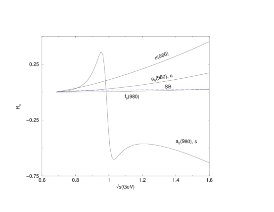
FIG. 3.: Individual contributions to $R(s)$ computed as for Fig. 2.

All in all, the essentially zero parameter prediction shown in Fig. 2 seems reasonable. Of course, satisfying the unitarity bound is a necessary rather than a sufficient condition for unitarity. To go further one may take different points of view. The simplest is to consider that our prediction is most accurate and just given for the real part of the amplitude. The motivation for this is that the tree graph approximation is purely real. Imaginary parts are introduced as regularizations like Eq. (4) in the vicinity of the resonance and may be regarded as (formally small) higher order effects. If we then choose to regard only $R(s)$ as predicted, we can satisfy unitarity by solving the unitarity formula $\left|S\right|=\left|\eta\right|$, which reads explicitly

$$R^{2}(s)+{\left[I(s)-\frac{1}{2}\right]}^{2}={\left[\frac{\eta(s)}{2}\right]}^{2},$$ (15)

for $I(s)$. The elasticity factor $\eta(s)$ may be taken to be approximately one. This procedure does not exactly solve the problem of finding an amplitude which satisfies both crossing symmetry and unitarity. While $R(s)$ coincides with the real part of the $l=0$ projection of the crossing symmetric Eq. (2), $I(s)$ obtained from Eq. (15) above does not coincide with the imaginary part of this projection. We note that the problem of constructing an invariant amplitude satisfying both crossing symmetry (Eq. (3)) and unitarity (Eq. (15)) for all its partial wave projections is an ancient and difficult one.

III More on Unitarity

In the preceding section we started from the crossing symmetric invariant amplitude Eq. (2) and regularized it according to the crossing symmetric prescription Eq. (4). There was no guarantee that its $l=0$ partial wave projection would be unitary or even satisfy the unitarity bounds. Fortunately the real part $R$ did satisfy the unitary bound and we could choose an imaginary part $I$ according to Eq. (15) such that partial wave unitarity in the $l=0$ channel was satisfied. This was at the expense of crossing symmetry for the imaginary part $I$. To see by how much the original amplitude Eq. (2) with the regularization Eq. (4) and its own imaginary part (i.e. the pure crossing symmetric case) violates unitarity, we have plotted $|S|$ in Fig. 4. It is seen that the unitarity violation in the elastic case (dashed line) is not very severe; this is due to the fact that the $a_{0}(980)$ resonance, which is approximately of Breit-Wigner shape, dominates.

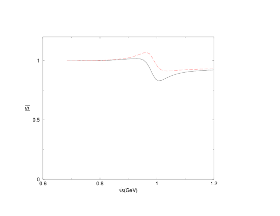
FIG. 4.: Unitarity of crossing symmetric S-matrix for $\pi\eta\rightarrow\pi\eta$ scattering. The dashed line corresponds to the elastic assumption, $G_{a_{0}}^{\prime}=65$ MeV in Eq. (4), while the solid line takes some inelasticity into account by setting $G_{a_{0}}^{\prime}=70$ MeV as explained in the text.

If $|R(s)|$ had turned out to be greater than $\displaystyle{\frac{1}{2}}$ at some values of $s$, we would have of course been unable to impose unitarity with the above method. It seems interesting to discuss a more or less conventional type of unitarization procedure which can be used in such a case. This operates at the level of the $l=0$ partial wave amplitude. We decompose the S-matrix into a piece associated with the $a_{0}$ resonance pole, $S_{pole}$, and a piece associated with the remaining “background” terms ($t$ and $u$-channel exchanges and contact term), $S_{B}$. The total S-matrix is written as the product

$$S\left(s\right) = S_{B}\left(s\right)S_{pole}\left(s\right)$$ (16)

$$= e^{2i\delta_{B}\left(s\right)}\frac{m_{a_{0}}^{2}-s+im_{a_{0}}\Gamma\left(s\right)}{m_{a_{0}}^{2}-s-im_{a_{0}}\Gamma\left(s\right)}.$$ (17)

In this form unitarity, $|S|=1$, is obvious. Now, using $S=1+2iT$ yields for the partial wave amplitude,

$$T\left(s\right) = T_{B}\left(s\right)+T_{pole}\left(s\right)$$ (18)

$$= e^{i\delta_{B}\left(s\right)}{\rm{sin}}\delta_{B}\left(s\right)+e^{2i\delta_{B}\left(s\right)}\frac{m_{a_{0}}\Gamma\left(s\right)}{m_{a_{0}}^{2}-s-im_{a_{0}}\Gamma\left(s\right)}.$$ (19)

For orientation, note that when the background phase $\delta_{B}$ vanishes and $\Gamma\left(s\right)$ is constant, this reduces to a pure Breit-Wigner form which is known to be unitary. If $\delta_{B}=\overline{{\delta_{B}}}$ and $\Gamma=\overline{\Gamma}$ are taken as constants we get the conventional local form [31] for a narrow resonance in a constant background:

$$T_{pole}\approx e^{2i\overline{\delta_{B}}}\frac{m_{a_{0}}\bar{\Gamma}}{m_{a_{0}}^{2}-s-im_{a_{0}}\bar{\Gamma}}.$$ (20)

As an example of an application of this last formula, we remark that the presence of a light $\sigma$ in $\pi\pi$ scattering produces [6] a background phase $\overline{\delta_{B}}\approx\displaystyle{\frac{\pi}{2}}$ near the $f_{0}(980)$. This results in an overall minus sign which converts the resonance peak into a dip. This is the same mechanism – the Ramsauer-Townsend effect – which was observed in atomic scattering [31] a long time ago.

Returning to the present case of elastic $\pi\eta$ scattering in the $l=0$ partial wave, we should, to get an exactly unitary amplitude, identify in Eq. (19)

$$\Gamma\left(s\right)=\frac{q}{32\pi m_{a}\sqrt{s}}\gamma_{a\pi\eta}^{2}{\left(s-m_{\pi}^{2}-m_{\eta}^{2}\right)}^{2},$$ (21)

where $q$ is the center of mass momentum. Furthermore, noting that $T_{B}(s)$ as obtained from the partial wave projection of the appropriate terms in Eq. (2) is purely real, we identify $\delta_{B}\left(s\right)$ from:

$$\frac{1}{2}{\rm{sin}}\left[2\delta_{B}\left(s\right)\right]=R_{B}\left(s\right).$$ (22)

In order that $T_{B}$ be unitary we must then manufacture an imaginary part from (22) as

$$I_{B}(s)={\rm{sin}}^{2}\left[\delta_{B}\left(s\right)\right].$$ (23)

The amplitude so constructed will satisfy $SS^{*}=1$ exactly but is, since among other things we have added $I_{B}\left(s\right)$ by hand, expected to violate crossing symmetry.

To summarize, we compare in Fig. 5 the real and imaginary parts of the $l=0$ projection of the crossing symmetric amplitude obtained in section II with the exactly unitary amplitude just discussed. It is encouraging for the method that the crossing symmetric but not exactly unitary amplitude is close to the unitary but not exactly crossing symmetric amplitude. Reasonably, the difference between the two curves gives a measure of the systematic uncertainties in the present method. Of course, there is no guarantee that the true solution lies between the two curves.

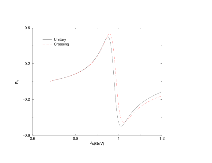
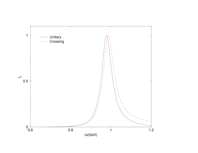
FIG. 5.: Comparison of the real and imaginary parts of the exactly crossing symmetric amplitude obtained in section II with the exactly unitary amplitude obtained in section III.

IV $\pi\eta$ scattering in the inelastic region

Here we give a start on extending the previous analysis to $\pi\eta$ scattering in the 1.2-1.6 GeV region, where the effects of inelastic channels, namely $\pi\eta\rightarrow K\bar{K}$ and $\pi\eta\rightarrow\pi{\eta}^{\prime}$, are expected to become important. For a full description we should use a coupled three-channel approach. According to our initially stated picture we should also include all of the resonance multiplets up to about 1.6 GeV as exchange particles. This amounts to a fairly large number of resonances (including some whose masses and decay properties are not yet firmly established) and suggests that such an ambitious program be postponed. In the present paper we shall survey the situation in analogy to an earlier treatment of $\pi K$ scattering in [8] by concentrating on the $\pi\eta\rightarrow\pi\eta$ channel. In the 1.2-1.6 GeV region the $a_{0}(1450)$ is the only scalar resonance in the direct channel. We shall also compute the $\pi\eta\rightarrow K\bar{K}$ and $\pi\eta\rightarrow\pi{\eta}^{\prime}$ amplitudes in our model, including the effects of the $a_{0}(1450)$. For these off-diagonal transitions we shall be mainly content to check unitarity.

Our approximation for the $\pi\eta\rightarrow\pi\eta$ amplitude up to about 1.6 GeV then consists of the sum of the amplitude given in section II and a piece associated with the $a_{0}(1450)$ resonance. The piece in section II is the $l=0$ partial wave projection of the invariant amplitude in Eq. (2), regularized according to Eq. (4). This gives an exactly crossing symmetric partial wave amplitude which we also saw in section III to be not very different from an exactly unitary partial wave amplitude. The regularized invariant amplitude including the $a_{0}(1450)$ is taken to be:

$$A_{\pi\eta}\left(s,t,u\right)\approx...+\frac{\gamma_{a^{\prime}\pi\eta}^{2}}{4}\frac{{\left(u-m_{\pi}^{2}-m_{\eta}^{2}\right)}^{2}}{m_{a^{\prime}}^{2}-u}+e^{2i\overline{\delta_{a^{\prime}}}}\frac{\gamma_{a^{\prime}\pi\eta}^{2}}{4}\frac{{\left(s-m_{\pi}^{2}-m_{\eta}^{2}\right)}^{2}}{m_{a^{\prime}}^{2}-s-im_{a^{\prime}}\Gamma_{tot}\left(a^{\prime}\right)},$$ (24)

where $a^{\prime}$ denotes the $a_{0}(1450)$ and the ellipsis stands for the other terms just mentioned. The coupling constants are related to the widths by an obvious generalization of Eq. (5). We have illustrated how to regularize the s-channel pole term as in (20) so as to maintain unitarity near where this term would have blown up. The phase $\overline{\delta_{a^{\prime}}}$ is evaluated from

$$\frac{1}{2}{\rm{sin}}\left[2\overline{\delta_{a^{\prime}}}\right]=R\left(s=m_{a^{\prime}}^{2}\right),$$ (25)

where $R(s)$ is the real part of the partial wave amplitude due to the background supplied by the regularized Eq. (2). We could multiply the u-channel term also by $e^{2i\overline{\delta_{a^{\prime}}}}$ to force crossing symmetry. Actually, we see from Fig. 2 that $R\left(s=m_{a^{\prime}}^{2}\right)$ is zero to good accuracy so this correction is not needed in the present case. Fig. 3 shows that this simplification arises because of cooperation between the pole and exchange terms. With $\overline{\delta_{a^{\prime}}}=0$, Eq. (24) is manifestly crossing symmetric (see the remark after Eq. (4)).

Note that Eq. (24) explicitly takes some account of inelasticity since $\Gamma_{tot}\left(a^{\prime}\right)=265\pm 13$ MeV [30] is not just gotten from the $a_{0}(1450)\rightarrow\pi\eta$ width as in the generalization of Eq. (5) but will be computed as

$$\Gamma_{tot}\left(a^{\prime}\right)\approx\Gamma_{\pi\eta}\left(a^{\prime}\right)+\Gamma_{K\bar{K}}\left(a^{\prime}\right)+\Gamma_{\pi{\eta}^{\prime}}\left(a^{\prime}\right).$$ (26)

This corresponds to the assumption that the $\pi\eta$, $K\bar{K}$ and $\pi{\eta}^{\prime}$ decay modes listed in [30] saturate the $a_{0}(1450)$ decay, although that assumption is not yet confirmed experimentally. If the experimental ratios [30]

$$\frac{\Gamma_{K\bar{K}}}{\Gamma_{\pi\eta}}=0.88\pm 0.23$$ (27)

and

$$\frac{\Gamma_{\pi{\eta}^{\prime}}}{\Gamma_{\pi\eta}}=0.35\pm 0.16$$ (28)

are taken together with this assumption we deduce:

$$\Gamma\left[a_{0}(1450)\rightarrow\pi\eta\right] \approx 119\pm 26\,{\rm{MeV}},$$ (29)

$$\Gamma\left[a_{0}(1450)\rightarrow K\bar{K}\right] \approx 105\pm 36\,{\rm{MeV}},$$ (30)

$$\Gamma\left[a_{0}(1450)\rightarrow\pi{\eta}^{\prime}\right] \approx 42\pm 23\,{\rm{MeV}}.$$ (31)

Actually these three partial widths should be related to each other by flavor SU(3) invariance. A best fit, on this assumption, yields the slightly different central values:

$$\Gamma^{\rm{SU}(3)}\left[a_{0}(1450)\rightarrow\pi\eta\right] \approx 155\,{\rm{MeV}},$$ (32)

$$\Gamma^{\rm{SU}(3)}\left[a_{0}(1450)\rightarrow K\bar{K}\right] \approx 86\,{\rm{MeV}},$$ (33)

$$\Gamma^{\rm{SU}(3)}\left[a_{0}(1450)\rightarrow\pi{\eta}^{\prime}\right] \approx 24\,{\rm{MeV}}.$$ (34)

A more detailed discussion of the $a_{0}(1450)$ decay modes is given in [27].

The real part of the $l=0$ partial wave amplitude is plotted up to 1.6 GeV using both Eq. (31) and Eq. (34) in Fig. 6. We see that these two cases are relatively close. Our prediction for the real part of the scattering amplitude naturally remains within the allowed range of -0.5 to 0.5 (except for a negligible deviation near the location of the $a_{0}(980)$). We have also plotted in Fig. 7 $\left|T_{11}\right|=\left|T\left(\pi\eta\rightarrow\pi\eta\right)\right|=\left|R_{11}+iI_{11}\right|$. This also is seen to satisfy the unitarity bound $\left|T_{11}\right|\leq 1$. It thus seems that the $\pi\eta\rightarrow\pi\eta$ scattering channel is remarkably simple in the approximation where the $a_{0}(1450)$ describes the inelastic region around 1.5 GeV. The partial wave $l=0$ amplitude is obtained as a projection of an exactly crossing symmetric invariant amplitude and the unitarity bounds are satisfied.

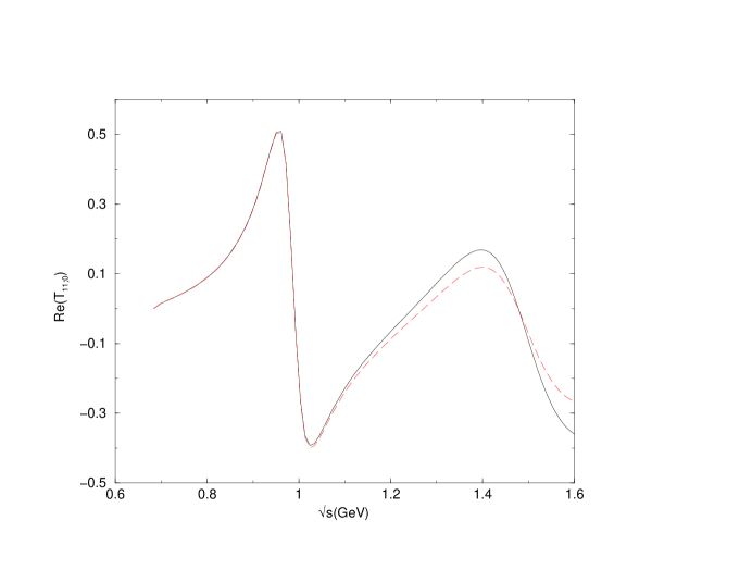
FIG. 6.: Our prediction for the real part of the $\pi\eta\rightarrow\pi\eta$ scattering amplitude up to 1.6GeV. The case where the decay properties of the $a_{0}(1450)$ are taken from Eq. (34) is represented by the solid line, and may be compared with the case using the estimate Eq. (31) shown by the dashed line.

FIG. 7.: Modulus of the $\pi\eta\rightarrow\pi\eta$ scattering amplitude.

V Off-diagonal channels

Now we present an initial study of the $\pi\eta\rightarrow K\bar{K}$ and $\pi\eta\rightarrow\pi{\eta}^{\prime}$ reactions in the energy range up to about 1.6 GeV. The Feynman diagrams needed to construct the $\pi\eta\rightarrow K\bar{K}$ invariant amplitude in our model are shown in Fig. 8.

FIG. 8.: Feynman diagrams representing the contributions to the $\pi\eta\rightarrow K\bar{K}$ scattering amplitude of (a) contact terms, (b) and (c) vector mesons, (d) and (e) strange scalar $\kappa(900)$ mesons and (f) $a_{0}(980)$ and $a_{0}(1450)$ mesons.

Unlike the preceding $\pi\eta\rightarrow\pi\eta$ case, vector meson exchanges and also contact terms arising from the first term of Eq. (A7) are now allowed. The contact contributions to the amplitude for $A_{\pi\eta\rightarrow K\bar{K}}\left(s,t,u\right)$ for ${\pi}^{+}\eta\rightarrow K^{+}\bar{K^{0}}$ from the first term of Eq. (A7) (“current-algebra” term) together with a piece from the third term of Eq. (A7) (due to addition of vector mesons in a chiral symmetric way) are:

$$\frac{2s-t-u}{3F_{\pi}^{2}}\left(\frac{{\rm cos}\theta_{p}}{\sqrt{2}}+{\rm sin}\theta_{p}\right)\left[1-\frac{3g_{\rho\pi\pi}^{2}F_{\pi}^{2}}{4m_{\rho}^{2}}\right].$$ (35)

The second term in the square bracket (from the vectors) is about 1.6 times the current algebra piece so it reverses the sign exactly as in the cases of $\pi\pi$ and $\pi K$ scattering [6, 7]. The contact amplitude arising from the pseudoscalar mass splittings in Eq. (A14) is

$${2\over{3F_{\pi}^{2}}}\left({\rm cos}\theta_{p}{{m_{\pi}^{2}+m_{K}^{2}}\over\sqrt{2}}-{\rm sin}\theta_{p}m_{K}^{2}\right),$$ (36)

and turns out to be completely negligible. The $K^{*}(890)$ exchange contributions shown in (b) and (c) of Fig. 8 are found to be

$$-\left({g_{\rho\pi\pi}\over 2}\right)^{2}\left({{{\rm cos}\theta_{p}}\over\sqrt{2}}+{\rm sin}\theta_{p}\right)\left[{{u-s+{{(m_{\pi}^{2}-m_{K}^{2})(m_{K}^{2}-m_{\eta}^{2})}\over{m_{K^{*}}^{2}}}}\over{m_{K^{*}}^{2}-t}}\right]+\left(t\leftrightarrow u\right).$$ (37)

The $\kappa(900)$ exchange contribution ((d) and (e) of Fig. 8) turns out to be negligible but arises from the amplitude piece

$${{\gamma_{\kappa K\pi}\gamma_{\kappa K\eta}}\over 4}\frac{(t-m_{\pi}^{2}-m_{K}^{2})(t-m_{K}^{2}-m_{\eta}^{2})}{m_{\kappa}^{2}-t}+\left(t\leftrightarrow u\right).$$ (38)

Finally, the s-channel contributions from the $a_{0}(980)$ and $a_{0}(1450)$, shown in (f) of Fig. 8, are being described by the regularized amplitude

$$\sum_{a}\,{{\gamma_{a\pi\eta}\gamma_{aKK}}\over 4}{{(s-2m_{K}^{2})(s-m_{\pi}^{2}-m_{\eta}^{2})}\over{m_{a}^{2}-s-im_{a}\Gamma^{tot}_{a}}},$$ (39)

where the sum is over $a=a_{0}(980)$ and $a_{0}(1450)$. The entire amplitude for $\pi\eta\rightarrow K\bar{K}$ is the sum of the terms above and is invariant under $t\leftrightarrow u$ exchange, as expected from charge conjugation invariance.

To proceed we have taken the projection of the amplitude into the $l=0$ partial wave using Eq. (6). The real parts of the non-negligible individual components are shown in Fig. 9. (Notice that the vertical scale has been greatly increased to accomodate the rather large individual contributions here). We see that the contact terms are dominant although they partially cancel each other.

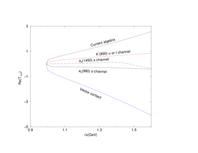
FIG. 9.: Real parts of contributions to the $l=0$ partial wave amplitude for $\pi\eta\rightarrow K\bar{K}$.

The total real part of the $\pi\eta\rightarrow K\bar{K}$ partial wave is shown in Fig. 10. Amusingly, all the large pieces in Fig. 9 collaborate with each other to satisfy the unitarity bound up to about 1.6 GeV. To test this further we included the imaginary parts of the partial wave amplitude, due to the regularization introduced in Eq. (39). The plot is shown in Fig. 11. It is seen that the stronger unitarity bound $\left|T_{12;0}\right|\leq\displaystyle{\frac{1}{2}}$ is violated only above 1.5 GeV.

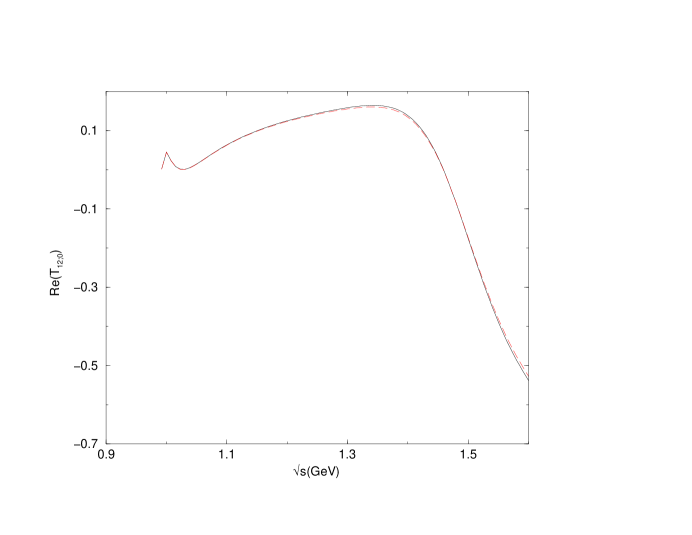
FIG. 10.: Real part of the total $l=0$ partial wave amplitude for $\pi\eta\rightarrow K\bar{K}$.

FIG. 11.: Plot of the magnitude of the $l=0$ partial wave amplitude for $\pi\eta\rightarrow K\bar{K}$.

Finally let us consider the $\pi\eta\rightarrow\pi{\eta}^{\prime}$ amplitude. The tree level Feynman diagrams are evident modifications of those shown in Fig. 1 for the $\pi\eta\rightarrow\pi\eta$ case. We have the regularized (due to the $a_{0}(980)$ and $a_{0}(1450)$ poles) tree amplitude

$$A_{\pi\eta\rightarrow\pi{\eta}^{\prime}}\left(s,t,u\right) = \sum_{r=\sigma,f_{0}(980)}\frac{\gamma_{r\pi\pi}\gamma_{r\eta{\eta}^{\prime}}}{\sqrt{2}}\frac{\left(t-2m_{\pi}^{2}\right)\left(t-m_{\eta}^{2}-m_{{\eta}^{\prime}}^{2}\right)}{m_{r}^{2}-t}+\frac{m_{\pi}^{2}}{F_{\pi}^{2}}{\rm{sin}}2\theta_{p}$$ (40)

$$+ \sum_{a}\frac{\gamma_{a\pi\eta}\gamma_{a\pi{\eta}^{\prime}}}{4}\left[\frac{\left(s-m_{\pi}^{2}-m_{\eta}^{2}\right)\left(s-m_{\pi}^{2}-m_{{\eta}^{\prime}}^{2}\right)}{m_{a}^{2}-s-im_{a}\Gamma_{a}^{tot}}\right.$$ (41)

$$+ \left.\frac{\left(u-m_{\pi}^{2}-m_{\eta}^{2}\right)\left(u-m_{\pi}^{2}-m_{{\eta}^{\prime}}^{2}\right)}{m_{a}^{2}-u}\right],$$ (42)

where the a-summation goes over $a_{0}(980)$ and $a_{0}(1450)$. The second term is a small contact correction due to the pseudoscalar meson mass splittings. The individual contributions to the $l=0$ partial wave projection of this amplitude are shown in Fig. 12 while the total $l=0$ projection is illustrated in Fig. 13. In this case, where the large contact terms are absent, the unitarity bound $\left|{\rm{Re}}T_{13;0}\right|\leq\frac{1}{2}$ is satisfied all the way up to 1.6 GeV. This also holds for the stronger bound, $\left|T_{13;0}\right|\leq\frac{1}{2}$, including the effects of the imaginary part as shown in the plot of Fig. 14. It is worthwhile to observe that the $a_{0}(1450)$ does not dominate either of the off-diagonal $\pi\eta\rightarrow K\bar{K}$ or $\pi\eta\rightarrow\pi{\eta}^{\prime}$ channels.

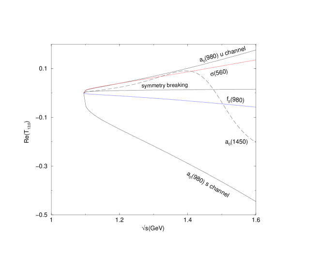
FIG. 12.: Real parts of individual contributions to the $l=0$ partial wave amplitudes for $\pi\eta\rightarrow\pi{\eta}^{\prime}$.

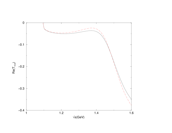
FIG. 13.: Real part of the total $l=0$ partial wave amplitude for $\pi\eta\rightarrow\pi{\eta}^{\prime}$.

FIG. 14.: Plot of the magnitude of the $l=0$ partial wave amplitude for $\pi\eta\rightarrow\pi{\eta}^{\prime}$.

Having looked at the individual $\pi\eta\rightarrow\pi\eta$, $\pi\eta\rightarrow K\bar{K}$ and $\pi\eta\rightarrow\pi{\eta}^{\prime}$ channels it is now interesting to check the unitarity relation for these l=0 S-matrix elements

$$\sum_{a}S_{1a;0}S_{1a;0}^{*}=1,$$ (43)

on the assumption that the two-particle channels completely saturate the s-wave $\pi\eta$ scattering at energies up to about 1.6 GeV. Expressing this formula in terms of the T-matrix elements suggests that we examine the deviation,

$$\Delta={\rm{Im}}\left(T_{11}\right)-{\left|T_{11}\right|}^{2}-{\left|T_{12}\right|}^{2}-{\left|T_{13}\right|}^{2}$$ (44)

which should vanish if Eq. (43) holds. This is plotted in Fig. 15.

FIG. 15.: Plot of $\Delta$, the deviation from unitarity for $\pi\eta$ scattering for $l=0$ channel. $\Delta=0$ for exact unitarity.

It is seen that our simple model yields, up until about 1.4 GeV, relatively small violations of unitarity for the s-wave amplitude. This state of affairs was obtained by projecting out the $l=0$ wave of an invariant amplitude which is exactly crossing symmetric. Thus the relative simplicity of $\pi\eta$ scattering enables one to come closer to obtaining an amplitude which is both crossing symmetric and unitary.

The larger violation of unitarity above 1.4 GeV can be seen to arise from the violation of the unitarity bounds already noticed in the $\pi\eta\rightarrow K\bar{K}$ amplitude (see Fig. 11). In turn this can be traced to the relatively large contact and vector meson terms which contribute to this particular off-diagonal process. This is in contrast to the $\pi\eta\rightarrow\pi\eta$ and $\pi\eta\rightarrow\pi{\eta}^{\prime}$ amplitudes for which the potentially large current algebra and vector meson terms were seen to vanish. Of course the large current algebra and vector meson pieces were very important in previous discussions of the $\pi\pi$ and $\pi K$ scatterings. In this sense, since they only enter through the “back door” of an off-diagonal channel for $\pi\eta$ scattering, the $\pi\eta$ scattering is effectively simpler to treat in our model.

Here, as mentioned above, we have just made an initial exploration of the coupled-channel $\pi\eta$ scattering problem. A fuller treatment would include the exchanges of spin 2 and other higher mass resonances and also scattering processes having $K\bar{K}$ and $\pi\eta^{\prime}$ initial states. For example important contributions in the $K\bar{K}$ case may be expected from the $K^{*}(1410)$.

VI Discussion

We studied $\pi\eta$ scattering in a model where the starting amplitude was computed at tree level from a phenomenological chiral Lagrangian containing exchanges of resonances having masses within the energy range of interest. Divergences at the direct channel poles were regularized in a conventional manner. Previously this method was applied to $\pi\pi$ scattering and $\pi K$ scattering; consistency required the existence of $\sigma(560)$ and $\kappa(900)$ scalar resonances. From that work and also from a related study of $\eta^{\prime}\rightarrow\eta\pi\pi$ decay, all the light scalar-pseudoscalar-pseudoscalar coupling constants were determined. These were used without change in the present work, which essentially involves no new parameters.

We first examined the roughly elastic region (up to about 1.2 GeV) which is dominated by the $a_{0}(980)$ resonance. It is noteworthy that neither vector mesons nor large “current algebra” contact terms can contribute in this region, unlike the $\pi\pi$ and $\pi K$ cases. The non-trivial contributions all arise from light scalar meson exchanges. Thus $\pi\eta$ scattering seems an excellent channel for learning more about these resonances which are of great current interest. Our model in section II was exactly crossing symmetric, but not exactly unitary. To see why that model which features an $a_{0}(980)$ with mass and width consistent with the experimental values is not automatically unitary we note the following two points: First, the amplitude is more general than a pure Breit-Wigner pole for the $a_{0}(980)$ s-channel since $\sigma$ and $f_{0}$ t-channel exchanges and $a_{0}(980)$ u-channel exchange also exist. Furthermore chiral symmetry dictates a non-trivial momentum dependence of the coupling factors.

To further investigate this question we constructed (in Section III) a related partial wave amplitude which we made unitary without regard for crossing symmetry. A comparison of the unitary and the crossing symmetric amplitudes showed that they were in fact close; the difference between them gives an estimate of the uncertainty of our approach.

It is encouraging to us that treating the $a_{0}(980)$ in $\pi\eta$ scattering by the same method as used in earlier discussions of $\pi\pi$ scattering (in which a $\sigma(560)$ and the $f_{0}(980)$ appeared) and $\pi K$ scattering (in which a $\kappa(900)$ was needed) seems to be reasonable. Now, all the members of a possible low-lying scalar nonet have been studied through their appearance in meson-meson scattering. Of course, many questions remain. One concerns the “family” structure of such a possible nonet; we have discussed some speculations on this aspect elsewhere [8, 27]. From the present viewpoint, the most important aspect concerns improving our understanding of the meson-meson chiral scattering amplitude. Clearly, one way to proceed is to examine the model at higher energies.

We thus made a preliminary exploration in section IV of the nearby inelastic region (roughly $1-1.5$ GeV). This range features the $a_{0}(1450)$ scalar resonance. It turns out that the earlier terms produce essentially zero background interference at the position of the $a_{0}(1450)$. Thus, it is natural to add this particle into the picture directly, yielding a crossing symmetric amplitude. This amplitude was seen to satisfy the unitarity bounds when the effects of inelasticity were incorporated in the regularization of the $a_{0}(1450)$ pole. The incomplete experimental data on the $a_{0}(1450)$ branching ratios were interpreted with the aid of a simple model. Similar preliminary discussions were given for the $\pi\eta\rightarrow K\bar{K}$ and $\pi\eta\rightarrow\pi{\eta}^{\prime}$ off-diagonal processes. An additional complication showed up in the $\pi\eta\rightarrow K\bar{K}$ case. Here the vector meson $K^{*}$ exchange and a large current algebra contact term both contribute as in the $\pi\pi$ and $\pi K$ scatterings. Nevertheless it was found that the exactly crossing symmetric amplitudes for $\pi\eta\rightarrow\pi\eta$, $K\bar{K}$ and $\pi{\eta}^{\prime}$ satisfied the unitarity relation amongst themselves to a reasonable accuracy until about 1.4 GeV.

There are many interesting directions for future work. Clearly a full 3-channel analysis and investigation of various alternative unitarization schemes is suggested. Inclusion of the many resonances in the $1-1.5$ GeV range which can be exchanged is also desirable. Especially interesting are the effects of the isoscalar scalars in this energy regime. Together with parallel expanded treatments of the $\pi\pi$ and $\pi K$ cases we may hope to learn about a second possible scalar nonet containing the $a_{0}(1450)$ and $K_{0}^{*}(1430)$. The knowledge of the scalar coupling constants obtained from refined analyses can be useful in the treatment of other physical processes. The recently measured [2] radiative decay $\phi(1020)\rightarrow a_{0}(980)+\gamma$ is especially important.

A Chiral Lagrangian

First we write the chiral Lagrangian of pseudoscalars and vectors. This makes use of the $3\times 3$ matrix $U=e^{2i\frac{\phi}{F_{\pi}}}$ wherein $\phi$ represents the usual $3\times 3$ matrix of pseudoscalar fields. Defining the square root $\xi$ by $U=\xi\xi$ we consider the combinations

$$p_{\mu} = \frac{i}{2}\left(\xi\partial_{\mu}\xi^{{\dagger}}-\xi^{{\dagger}}\partial_{\mu}\xi\right)\ ,$$ (A1)

$$v_{\mu} = \frac{i}{2}\left(\xi\partial_{\mu}\xi^{{\dagger}}+\xi^{{\dagger}}\partial_{\mu}\xi\right)\ .$$ (A2)

Under a chiral transformation $U\rightarrow U_{\rm L}UU_{\rm R}^{{\dagger}}$, $\xi$ transforms as:

$$\xi\rightarrow U_{\rm L}\,\xi\,K^{{\dagger}}(\phi,U_{\rm L},U_{\rm R})=K(\phi,U_{\rm L},U_{\rm R})\,\xi\,U_{\rm R}^{{\dagger}},\$$ (A3)

which defines $K(\phi,U_{\rm L},U_{\rm R})$. A vector meson nonet $\rho_{\mu}$ transforms as a gauge field

$$\rho_{\mu}\rightarrow K\rho_{\mu}K^{{\dagger}}+\frac{i}{\widetilde{g}}K\partial_{\mu}K^{{\dagger}}.$$ (A4)

Similarly

$$v_{\mu}\rightarrow Kv_{\mu}K^{{\dagger}}+iK\partial_{\mu}K^{{\dagger}},$$ (A5)

while

$$p_{\mu}\rightarrow Kp_{\mu}K^{{\dagger}}.$$ (A6)

The chiral invariant (neglecting quark mass induced terms) Langrangian of pseudoscalars and vectors may then be written as

$${\cal L}_{1}=-\frac{F_{\pi}^{2}}{8}{\rm{Tr}}\left(\partial_{\mu}U{\partial_{\mu}U}^{\dagger}\right)-\frac{1}{4}\mbox{Tr}\left[F_{\mu\nu}(\rho)F_{\mu\nu}(\rho)\right]-\frac{1}{2}m_{\rho}^{2}\mbox{Tr}\left(\rho_{\mu}-\frac{v_{\mu}}{\widetilde{g}}\right)^{2}-\frac{m_{0}^{2}F_{\pi}^{2}}{96}{\left({\rm{ln}}\frac{{\rm{det}}U}{{\rm{det}}{U}^{\dagger}}\right)}^{2},$$ (A7)

where $F_{\mu\nu}=\partial_{\mu}\rho_{\nu}-\partial_{\nu}\rho_{\mu}-i\widetilde{g}[\rho_{\mu},\rho_{\nu}]$ is the vector meson gauge field strength. $F_{\pi}=0.131$ GeV is the pion decay constant, $\tilde{g}$ is the vector meson gauge coupling constant and $m_{0}$ is a mass for the unmixed ${\eta}^{\prime}$ field. $\tilde{g}$ is related to the $\rho$ meson width by

$$\Gamma\left(\rho\rightarrow\pi\pi\right)=\frac{g_{\rho\pi\pi}^{2}{q_{\pi}^{3}}}{12\pi m_{\rho}^{2}}\quad,\quad g_{\rho\pi\pi}=\frac{m_{\rho}^{2}}{\tilde{g}F_{\pi}^{2}}\approx 8.56$$ (A8)

and $m_{\rho}=0.77$ GeV. $q_{\pi}$ is the pion momentum in the rest frame of the decaying $\rho$ meson. The last term in Eq. (A7) reflects the $U\left(1\right)_{A}$ anomaly in QCD and allows the ${\eta}^{\prime}$ particle to have a suitably large mass. We take $m_{\pi}=0.137$ GeV, $m_{K}=0.496$ GeV, $m_{\eta}=0.547$ GeV, $m_{{\eta}^{\prime}}=0.958$ GeV and $m_{K^{*}}=0.890$ GeV.

Next consider the chiral invariant Lagrangian involving the scalar nonet field $N$. We note [32] that $N$ may be taken to transform as

$$N\rightarrow KNK^{\dagger}.$$ (A9)

Then it is clear that

$${\cal L} = -\frac{1}{2}{\rm Tr}\left({\cal D}_{\mu}N{\cal D}_{\mu}N\right)-a{\rm Tr}\left(NN\right)-c{\rm Tr}\left(N\right){\rm Tr}\left(N\right)+F_{\pi}^{2}\left[A\epsilon^{abc}\epsilon_{def}N_{a}^{d}{\left(p_{\mu}\right)}_{b}^{e}{\left(p_{\mu}\right)}_{c}^{f}\right.$$ (A10)

$$+ \left.B{\rm Tr}\left(N\right){\rm Tr}\left(p_{\mu}p_{\mu}\right)+C{\rm Tr}\left(Np_{\mu}\right){\rm Tr}\left(p_{\mu}\right)+D{\rm Tr}\left(N\right){\rm Tr}\left(p_{\mu}\right){\rm Tr}\left(p_{\mu}\right)\right],$$ (A11)

where ${\cal D}=\partial_{\mu}-iv_{\mu}$, is chirally invariant. The coupling constants describing scalar $\rightarrow$ pseudoscalar $+$ pseudoscalar are given in terms of the coefficients $A$, $B$, $C$ and $D$; these were determined from $\pi\pi$ scattering, $\pi K$ scattering and ${\eta}^{\prime}\rightarrow\eta\pi\pi$ decay in [8, 9]. As an explicit example of a coupling constant describing a trilinear interaction among isomultiplets extracted from Eq. (A11) consider

$$-{\cal L}_{N\phi\phi}=\frac{\gamma_{\kappa K\pi}}{\sqrt{2}}\left(\partial_{\mu}{\bar{K}}\mbox{\boldmath${\tau}$}\cdot\partial_{\mu}{\mbox{\boldmath${\pi}$}}\kappa+h.c.\right)+...,$$ (A12)

which yields the identification $\gamma_{\kappa K\pi}=-2A$. The other terms in this isotopic spin decomposition are also given in [8].

Symmetry breaking terms must still be added. These involve the “spurion” matrix

$${\cal M}={\rm diag}\left(1,1,x\right)$$ (A13)

where $x\approx 20.5$ [33] is the strange to nonstrange quark mass ratio. Pseudoscalar mass terms are propotional to

$${\rm Tr}\left(U{\cal M}^{\dagger}\right)+h.c.,$$ (A14)

vector mass splitting terms are contained in a term

$${\rm Tr}\left[{\xi}^{\dagger}{\cal M}\xi^{\dagger}{\left(\tilde{g}\rho_{\mu}-v_{\mu}\right)}^{2}\right]+h.c.$$ (A15)

and finally scalar meson mass splittings are contained in:

$$-\frac{b}{2}{\rm Tr}\left(NN\xi^{\dagger}{\cal M}\xi^{\dagger}\right)+\frac{d}{2}{\rm Tr}\left(N\right){\rm Tr}\left(N\xi^{\dagger}{\cal M}\xi^{\dagger}\right)+h.c.$$ (A16)

A detailed discussion of the scalar meson mass terms and the determination of the parameters $a$, $b$, $c$ and $d$ was given in [8].

The main effects of these mass splitting terms are to give each particle its correct experimental mass and to accomodate mixing between particles of the same spin-parity and isospin. Our conventions for the $\eta-{\eta}^{\prime}$ and $\sigma-\sigma^{\prime}$ mixing are:

$$\left(\begin{array}[]{c}\eta\\ \eta^{\prime}\end{array}\right)=\left(\begin{array}[]{c c}{\rm cos}\theta_{p}&-{\rm sin}\theta_{p}\\ {\rm sin}\theta_{p}&{\rm cos}\theta_{p}\end{array}\right)\left(\begin{array}[]{c}(\phi^{1}_{1}+\phi^{2}_{2})/\sqrt{2}\\ \phi^{3}_{3}\end{array}\right)$$ (A17)

and

$$\left(\begin{array}[]{c}\sigma\\ f_{0}\end{array}\right)=\left(\begin{array}[]{c c}{\rm cos}\theta_{s}&-{\rm sin}\theta_{s}\\ {\rm sin}\theta_{s}&{\rm cos}\theta_{s}\end{array}\right)\left(\begin{array}[]{c}N_{3}^{3}\\ \frac{N_{1}^{1}+N_{2}^{2}}{\sqrt{2}}\end{array}\right).$$ (A18)

The asymmetry in these two definitions reflects the prejudice that in the ideal mixing limit (zero mixing angle) the heaviest pseudoscalar $\eta^{\prime}$ is identified as $\phi_{3}^{3}$ while the lightest scalar $\sigma$ is identified as $N^{3}_{3}$. We choose the conventional value $\theta_{p}=37^{o}$ and a value $\theta_{s}=-20.3^{o}$ as discussed in [8]. This corresponds to the scalar meson masses (needed to explain $\pi\pi$ and $\pi K$ scattering in our model):

$$m_{\sigma}=550\,{\rm MeV}\,\, \,\,m_{f_{0}}=980\,{\rm MeV}$$ , (A19)

$$m_{a_{0}}=983.5\,{\rm MeV}\,\, \,\,m_{\kappa}=897\,{\rm MeV}.$$ , (A20)

We take the heavier scalar isovector to have a mass given by [30], namely $m[a_{0}(1450)]=1.474$ GeV. The coupling constants for the light scalars to two pseudoscalars relevant for the present paper are (in units of ${\rm{GeV}}^{-1}$) [8, 9]:

$$\gamma_{\sigma\pi\pi}=7.27\,\, \,\,\gamma_{\sigma\eta\eta}=4.11\,\,,\,\,\gamma_{\sigma\eta{\eta}^{\prime}}=2.65$$ , (A21)

$$\gamma_{f_{0}\pi\pi}=1.47\,\, \,\,\gamma_{f_{0}\eta\eta}=1.72\,\,,\,\,\gamma_{f_{0}\eta{\eta}^{\prime}}=-9.01$$ , (A22)

$$\gamma_{a_{0}\pi\eta}=-6.80\,\, \,\,\gamma_{a_{0}K\bar{K}}=-5.02\,\,,\,\,\gamma_{a_{0}\pi{\eta}^{\prime}}=-7.80$$ , (A23)

$$\gamma_{\kappa K\pi} =-5.02\,\,,\gamma_{\kappa K\eta}=-0.94$$ (A24)

B Partial wave projection of $\pi\eta\rightarrow\pi\eta$ elastic amplitude

The s-wave projections of the invariant amplitudes represented in Fig. 1 are calculated from the $l=0$ and $a=b=1$ case of Eq. (6). The direct channel s-wave amplitude is:

$$T_{11;0}^{s-channel}=\rho(s)\frac{{\gamma_{a_{0}\pi\eta}}^{2}}{2}\frac{{\left(s-m_{\pi}^{2}-m_{\eta}^{2}\right)}^{2}}{m_{a_{0}}^{2}-s-im_{a_{0}}G_{a_{0}}^{\prime}\theta\left[s-{\left(m_{\eta}+m_{\pi}\right)}^{2}\right]},$$ (B1)

where $\rho(s)\equiv\rho_{1}(s)$ in the notation of Eq. (7) for channel 1 ($\pi\eta\rightarrow\pi\eta$). The projection of the t-channel amplitude of Fig. 1(a) is:

$$T_{11;0}^{t-channel,r}=\rho(s)q^{2}\frac{\gamma_{r\pi\pi}\gamma_{r\eta\eta}}{\sqrt{2}}\left[2\alpha-4\gamma+\left(\alpha\gamma-\beta-2\gamma^{2}\right){\rm{ln}}\left|\frac{\gamma-1}{\gamma+1}\right|\right],$$ (B2)

where $q^{2}$ is the center of mass momentum and

$$\alpha\equiv 2\frac{m_{\pi}^{2}+m_{\eta}^{2}+2q^{2}}{q^{2}}\,,\,\beta\equiv 2\frac{\left(m_{\pi}^{2}+q^{2}\right)\left(m_{\eta}^{2}+q^{2}\right)}{q^{4}}\,,\,\gamma\equiv\frac{m_{r}^{2}+2q^{2}}{2q^{2}}.$$ (B3)

Here there is one term with $r=\sigma$ and another with $r=f_{0}(980)$. Finally, the $l=0$ projection of the $a_{0}(980)$ u-channel exchange amplitude is:

$$T_{11;0}^{u-channel}=\rho(s)q^{2}\frac{{\gamma_{a\pi\eta}}^{2}}{2}\left[2B+4C+C^{2}{\rm{ln}}\left|\frac{B+1}{B-1}\right|\right],$$ (B4)

where

$$B\equiv\frac{1}{2q^{2}}\left[m_{a}^{2}-m_{\eta}^{2}-m_{\pi}^{2}+2\sqrt{m_{\pi}^{2}+q^{2}}{\sqrt{m_{\eta}^{2}+q^{2}}}\right]\equiv\frac{{\sqrt{m_{\pi}^{2}+q^{2}}}{\sqrt{m_{\eta}^{2}+q^{2}}}}{q^{2}}-C.$$ (B5)

REFERENCES

- [1] R.L. Jaffe, Phys. Rev. D15, 267 (1977);
- [2] M.N. Achasov et al, Phys. Lett. B 440, 442 (1998) and very recently R.R. Akhmetshin et al, Report Budker INP 99-11, 1999 and also E.P. Solodov, Talk at “International Workshop on collisions from to J/, Budker Institute of Nuclear Physics, Novosibirsk, Russia, March 1-5, 1999.
- [3] N.N. Achasov, Phys.Usp. 41, 1149 (1998). See also N.N. Achasov and V.V. Gubin,, Phys. Rev. D 56, 4048 (1997) and N.N. Achasov and V.N. Ivanchenko, Nucl. Phys. B315(1989) 465-476.
- [4] See also F.E. Close, N. Isgur and S. Kumano, Nucl. Phys. B389 (1993) 513-533
- [5] N. Isgur and J. Weinstein, Phys. Rev. Lett 48, 659 (1982); Phys. Rev. D27 588 (1983)
- [6] F. Sannino and J. Schechter, Phys. Rev. D52, 96 (1995) and M. Harada, F. Sannino and J. Schechter, Phys. Rev. D54, 1991 (1996), Phys. Rev. Lett. 78, 1603 (1997).
- [7] D. Black, A.H. Fariborz, F. Sannino and J. Schechter, Phys. Rev. D58, 054012 (1998).
- [8] D. Black, A.H. Fariborz, F. Sannino and J. Schechter, Phys. Rev. D59, 074026 (1999).
- [9] A.H. Fariborz and J. Schechter, Phys. Rev. D60, 034002 (1999).
- [10] See N.A. Törnqvist, Z. Phys. C68, 647 (1995) and references therein. In addition see N.A. Törnqvist and M. Roos, Phys. Rev. Lett. 76, 1575 (1996), N.A. Törnqvist, hep-ph/9711483 and Phys. Lett. B426 105 (1998).
- [11] S. Ishida, M.Y. Ishida, H. Takahashi, T. Ishida, K. Takamatsu and T Tsuru, Prog. Theor. Phys. 95, 745 (1996), S. Ishida, M. Ishida, T. Ishida, K. Takamatsu and T. Tsuru, Prog. Theor. Phys. 98, 621 (1997). See also M. Ishida and S. Ishida, Talk given at 7th International Conference on Hadron Spectroscopy (Hadron 97), Upton, NY, 25-30 Aug. 1997, hep-ph/9712231.
- [12] D. Morgan and M. Pennington, Phys. Rev. D48, 1185 (1993).
- [13] G. Janssen, B.C. Pearce, K. Holinde and J. Speth, Phys. Rev. D52, 2690 (1995).
- [14] A.A. Bolokhov, A.N. Manashov, M.V. Polyakov and V.V. Vereshagin, Phys. Rev. D48, 3090 (1993). See also V.A. Andrianov and A.N. Manashov, Mod. Phys. Lett. A8, 2199 (1993). Extension of this string-like approach to the case has been made in V.V. Vereshagin, Phys. Rev. D55, 5349 (1997) and very recently in A.V. Vereshagin and V.V. Vereshagin, ibid. 59, 016002 (1999) which is consistent with a light state.
- [15] N.N. Achasov and G.N. Shestakov, Phys. Rev. D49, 5779 (1994).
- [16] R. Kamínski, L. Leśniak and J. P. Maillet, Phys. Rev. D50, 3145 (1994).
- [17] M. Svec, Phys. Rev. D53, 2343 (1996).
- [18] E. van Beveren, T.A. Rijken, K. Metzger, C. Dullemond, G. Rupp and J.E. Ribeiro, Z. Phys. C30, 615 (1986). E. van Beveren and G. Rupp, hep-ph/9806246, 248. See also J.J. de Swart, P.M.M. Maessen and T.A. Rijken, U.S./Japan Seminar on the YN Interaction, Maui, 1993 [Nijmegen report THEF-NYM 9403].
- [19] R. Delbourgo and M.D. Scadron, Mod. Phys. Lett. A10, 251 (1995). See also D. Atkinson, M. Harada and A.I. Sanda, Phys. Rev. D46, 3884 (1992).
- [20] J.A. Oller, E. Oset and J.R. Pelaez, Phys. Rev. Lett. 80, 3452 (1998). See also K. Igi and K. Hikasa, Phys. Rev. D59, 034005 (1999).
- [21] A.V. Anisovich and A.V. Sarantsev, Phys. Lett. B413, 137 (1997).
- [22] V. Elias, A.H. Fariborz, Fang Shi and T.G. Steele, Nucl. Phys. A633, 279 (1998).
- [23] V. Dmitrasinović, Phys. Rev. C53, 1383 (1996).
- [24] P. Minkowski and W. Ochs, hep-ph/9811518.
- [25] S. Godfrey and J. Napolitano, hep-ph/9811410.
- [26] L. Burakovsky and T. Goldman, Phys. Rev. D57 2879 (1998)
- [27] D. Black, A.H. Fariborz, J. Schechter, hep-ph/9907516
- [28] E. Witten, Nucl. Phys. B160, 57 (1979). See also S. Coleman, Aspects of Symmetry, Cambridge University Press (1985). The original suggestion is given in G. ’t Hooft, Nucl. Phys. B72, 461 (1974).
- [29] S. Teige et al, Phys. Rev. D59 012001 (1999)
- [30] Review of Particle Physics, Euro. Phys. J C3 (1999).
- [31] J. R. Taylor, Scattering Theory, Krieger (1987).
- [32] C. Callan, S. Coleman, J. Wess and B. Zumino, Phys. Rev. 177, 2247 (1969).
- [33] See for example M. Harada and J. Schechter, Phys. Rev. D54, 3394 (1996)