UT-850
The Auxiliary Mass Method beyond the Local Potential Approximation

We show that the evolution equation of the effective potential in the auxiliary mass method corresponds to a leading approximation of a certain series. This series is derived from an evolution equation of an effective action using a derivative expansion. We derived an expression of the next-to-leading approximation of the evolution equation, which is a simultaneous partial differential equation.

1 Introduction

Finite temperature field theory, which is based only on the statistical mechanism, adequately describes many physical phenomena such as phase transitions and mass spectrum in a thermal bath[1, 2, 3]. Its perturbation theory, however, breaks down at a high finite temperature. Mass squared becomes negative even in a vacuum at the finite temperature. This problem is solved by the ring resummation, which adds thermal mass to zero temperature mass beforehand[4, 5]. This procedure is still insufficient yet to make the perturbative expansion be reliable, especially around the critical temperature. For example, the perturbation theory indicates that the phase transition of the $Z_{2}$-invariant scalar theory is of first order incorrectly[6]. For the other example, different properties are indicated by the perturbation theory and lattice simulations in investigations of the Abelian Higgs model[4, 7, 8, 9, 10, 11, 12, 13, 14, 15] and the Standard model[16, 17, 18, 19, 20, 21, 22, 23, 24] at large Higgs boson mass range.

These failure of the perturbation theory is caused by bad infrared behavior around the critical temperature[25, 26]. A loop expansion parameter becomes $\lambda T/m$ even after the ring resummation due to this infrared effect. Here $\lambda$ is a small coupling constant and $m$ is mass at the temperature $T$. The perturbation theory is, therefore, unreliable at a high temperature and small mass. This situation arises around the critical temperature of second order phase transitions or weakly first order phase transitions. The auxiliary mass method controls this infrared behavior by introducing ”auxiliary mass”[27, 28, 29, 30, 31, 32]. We first calculate an effective potential with the large auxiliary mass, $M\sim T$. This effective potential is reliable since the loop expansion parameter is small thanks to the auxiliary mass. We next calculate the effective potential at true mass from this effective potential through an evolution equation. We solve the evolution equation of the effective potential with respect to variation of mass squared.

We used a certain approximation to derive the evolution equation in Ref.[28, 29]. Though we got quite good results using the approximation, we did not have methods to improve the approximation. In the present paper, we show that the previous evolution equation is a leading approximation of a certain series. We then derive a next-to-leading evolution equation, which is a simultaneous partial differential equation. Though it is difficult to solve the evolution equation at an arbitrary temperature due to numerical problems, we can, in principle, improve the approximation systematically.

2 Evolution Equation

In this section, we explain our idea and derive the evolution equation for the $Z_{2}$-invariant scalar theory using the auxiliary mass method. Let’s consider the following Euclidean Lagrangian density with mass squared $m^{2}$,

$${\cal L}_{E}(\phi;m^{2})=-\frac{1}{2}\left(\frac{\partial\phi}{\partial\tau}\right)^{2}-\frac{1}{2}(\mbox{\boldmath$\nabla$}\phi)^{2}-\frac{1}{2}m^{2}\phi^{2}-\frac{\lambda}{4!}(\phi^{2})^{2}+J_{m}\phi+c.t.\ .$$ (1)

Here $J_{m}(x)$ is an external source function which sets

$$<\phi(x)>=\phi_{c}(x)$$ (2)

and hence depends on $m^{2}$. We set true mass squared negative, $m^{2}=-\mu^{2}$, since we investigate the phase transition of this theory. We assume that the coupling constant $\lambda$ is small so that the perturbation theory be reliable at a low temperature ($T\ll m$).

Our idea is the following. The effective action for the theory, $\Gamma[\phi_{c};m^{2})$, satisfies the following identity,

$$\Gamma[\phi_{c};-\mu^{2})=\int^{-\mu^{2}}_{M^{2}}\left(\frac{\partial\Gamma[\phi_{c};m^{2})}{\partial m^{2}}\right)dm^{2}+\Gamma[\phi_{c};M^{2}).$$ (3)

We set $M^{2}$ so large ($\sim T^{2}$) that we can calculate the initial condition, $\Gamma[\phi_{c};M^{2})$, reliably by the perturbation theory. If we can evaluate the derivative ${\partial\Gamma(\phi_{c})}/{\partial m^{2}}$ correctly, we can calculate the effective action accurately.

2.1 Derivative of the effective action with respect to mass squared

In this subsection we calculate the derivative $\frac{\partial\Gamma[\phi_{c}]}{\partial m^{2}}$. This is formally given by[28, 29],

$$\frac{\partial\Gamma[\phi_{c}]}{\partial m^{2}} = -\frac{1}{2}\int d^{4}x<\phi(x)^{2}>$$

$$= -\frac{1}{2}\int d^{4}xd^{4}y<\phi(x)\phi(y)>\delta(y-x)$$

$$= -\frac{1}{2}\int d^{4}x\phi_{c}(x)^{2}-\frac{1}{2}\int d^{4}xd^{4}y\left(\frac{\delta^{2}(-\Gamma[\phi_{c}])}{\delta\phi_{c}(x)\delta\phi_{c}(y)}\right)^{-1}\delta(y-x),$$

here “$\int d^{4}x$” is an abbreviation of “$\int^{\beta}_{0}d\tau\int_{-\infty}^{\infty}d^{3}x$”. We use this notation from now on.

Since Eq.(2.1) is a functional equation, it can not be solved directly. We, therefore, limit functional space and expand $\Gamma[\phi_{c}]$ in powers of derivatives[33, 34],

$$\Gamma[\phi_{c}]=\int d^{4}x\left[-V(\phi_{c}^{2})-\frac{1}{2}K_{0}(\phi_{c}^{2})(\partial_{0}\phi_{c})^{2}-\frac{1}{2}K_{s}(\phi_{c}^{2})(\nabla\phi_{c})^{2}+\cdots\right],$$ (5)

where $\cdots$ denotes terms with higher derivative. Note that the coefficient functional of $(\partial_{0}\phi_{c})^{2}$ differs from that of $(\nabla\phi_{c})^{2}$ due to absence of the 4-dimensional Euclidean symmetry. We then expand the both side of Eq.(2.1) with respect to derivative as Eq.(5) and match the coefficient functionals of each terms. In practice, we have to truncate the series in Eq.(5) at finite terms. In the present paper, we leave the three terms in Eq.(5). This is the next-to-leading approximation of the derivative expansion. We obtain the leading approximation, which corresponds to the evolution equation of the previous paper Ref[28, 29], by taking $K_{0}=1$ and $\ K_{s}=1$

From Eq.(5), l.h.s of Eq.(2.1) becomes,

$$-\frac{\partial\Gamma}{\partial m^{2}}=\int d^{4}x\left[\frac{\partial V}{\partial m^{2}}+\frac{1}{2}\frac{\partial K_{0}}{\partial m^{2}}(\partial_{0}\phi_{c})^{2}+\frac{1}{2}\frac{\partial K_{s}}{\partial m^{2}}(\nabla\phi_{c})^{2}\right].$$ (6)

From Eq.(5), up to the second derivative terms,

$$M_{yx} \equiv -\frac{\delta^{2}\Gamma[\phi_{c}]}{\delta\phi_{c}(x)\delta\phi_{c}(y)}$$

$$= \delta(y-x)\left[V^{{}^{\prime\prime}}(\phi_{c}(y))\right.$$

$$-\left\{\frac{1}{2}K_{0}^{{}^{\prime\prime}}(\phi_{c}(y))(\partial_{0}\phi_{c}(y))^{2}+K_{0}^{{}^{\prime}}(\phi_{c}(y))\partial_{0}\phi_{c}(y)\partial_{y_{0}}\right.$$

$$\left.+K_{0}^{{}^{\prime}}(\phi_{c}(y))\partial_{0}^{2}\phi_{c}(y)+K_{0}(\phi_{c}(y))\partial_{y_{0}}^{2}\right\}$$

$$\left.-\left\{K_{0}\leftrightarrow K_{s},\partial_{y_{0}}\leftrightarrow\nabla_{y}\right\}\right].$$

$$= \delta(y-x)(-\overline{K}_{0}\partial_{y_{0}}^{2}-\overline{K}_{s}\nabla_{y}^{2}+\overline{V}^{\prime\prime})$$

$$+\delta(y-x)\left[{\widetilde{V}^{{}^{\prime\prime}}(\phi_{c}(y))}\right.$$

$$-\left\{\frac{1}{2}K_{0}^{{}^{\prime\prime}}(\phi_{c}(y))(\partial_{0}\phi_{c}(y))^{2}+K_{0}^{{}^{\prime}}(\phi_{c}(y))\partial_{0}\phi_{c}(y)\partial_{y_{0}}\right.$$

$$+\left.K_{0}^{{}^{\prime}}(\phi_{c}(y))\partial_{0}^{2}\phi_{c}(y)+\widetilde{K}_{0}(\phi_{c}(y))\partial_{y_{0}}^{2}\right\}$$

$$-\left.\left\{K_{0}\leftrightarrow K_{s},\partial_{y_{0}}\leftrightarrow\nabla_{y}\right\}\right]$$

$$= A_{yx}-B_{yx},$$ (9)

$$A_{yx} \equiv \delta(y-x)(-\overline{K}_{0}\partial_{y_{0}}^{2}-\overline{K}_{s}\nabla_{y}^{2}+\overline{V}^{\prime\prime})$$

$$B_{yx} \equiv A_{yx}-M_{yx}$$

$$\widetilde{V}^{{}^{\prime\prime}}(\phi_{c}(y)) \equiv V^{{}^{\prime\prime}}(\phi_{c}(y))-\overline{V}^{{}^{\prime\prime}}$$

$$\widetilde{K}_{0}(\phi_{c}(y)) \equiv K_{0}(\phi_{c}(y))-\overline{K}_{0}$$

Here, we divide $M_{yx}$ into two parts, $A_{yx}$ and $B_{yx}$, which remains finite and vanishes at $\phi_{c}(x)=\bar{\phi}$ respectively. Details of the following calculation are explained in the appendix. The right hand side of Eq.(2.1) can now be expanded around $\phi_{c}(x)=\bar{\phi}$ up to the second derivative as follows,

$$\int d^{4}xd^{4}y(\frac{\delta^{2}(-\Gamma[\phi_{c}])}{\delta\phi_{c}(x)\delta\phi_{c}(y)})^{-1}\delta(y-x)$$

$$= \int d^{4}x(A^{-1})_{xx}$$

$$+\int d^{4}xd^{4}yd^{4}z(A^{-1})_{xy}B_{yz}(A^{-1})_{zx}$$

$$+\int d^{4}xd^{4}yd^{4}zd^{4}ud^{4}v(A^{-1})_{xy}B_{yz}(A^{-1})_{zu}B_{uv}(A^{-1})_{vx}$$

$$+\cdots$$

$$= \int_{px}\frac{1}{\nu}$$

$$+\int_{px}\frac{1}{\nu^{2}}\left[-\frac{1}{2}\left\{\overline{K}_{0}^{\prime\prime}(\partial_{0}\phi_{c})^{2}+\overline{K}_{s}^{\prime\prime}(\nabla\phi_{c})^{2}\right\}\right]$$

$$+\int_{px}\frac{1}{\nu^{3}}\left[\left\{\overline{K}_{0}^{\prime}p_{0}(\partial_{0}\phi_{c})+\overline{K}_{s}^{\prime}p_{i}(\partial_{i}\phi_{c})\right\}^{2}\right.$$

$$\ \ \ \ \ \ \ \ \ \left.+\ 2\left\{\overline{K}^{\prime}_{0}(\partial_{0}\phi_{c})^{2}+\overline{K}^{\prime}_{s}(\nabla\phi_{c})^{2}\right\}\nu^{\prime}\right]$$

$$\int_{px}\frac{1}{\nu^{4}}\left[-2\left\{\overline{K}_{0}^{\prime}p_{0}\partial_{0}\phi_{c}+\overline{K}_{s}^{\prime}p_{i}\partial_{i}\phi_{c}\right\}\left\{\overline{K}_{0}p_{0}\partial_{0}\phi_{c}+\overline{K}_{s}p_{i}\partial_{i}\phi_{c}\right\}\nu^{\prime}\right.$$

$$\left.\ \ \ \ \ \ \ -\frac{1}{2}\left\{\nu^{\prime}\right\}^{2}\left\{\overline{K}_{0}(\partial_{0}\phi_{c})^{2}+\overline{K}_{s}(\nabla\phi_{c})^{2}\right\}\right]$$

$$+\cdots+(terms\ which\ vanish\ at\ \phi_{c}(x)=\bar{\phi}\ like\ \widetilde{V}\times(something)),$$

where $\nu=\overline{K}_{0}p_{0}^{2}+\overline{K}_{s}{\bf p}^{2}+\overline{V}^{\prime\prime}$, $\nu^{\prime}=\overline{K}^{\prime}_{0}p_{0}^{2}+\overline{K}^{\prime}_{s}{\bf p}^{2}+\overline{V}^{\prime\prime\prime}$ (with $p_{0}=2\pi nT(n=0,\pm 1,\cdots)$ and ${\bf p}^{2}\equiv\sum_{i=1}^{3}p_{i}^{2}$) and “$\int_{px}$” is an abbreviation of “$T\sum_{n=-\infty}^{\infty}\int d^{3}p/(2\pi)^{3}\int d^{4}x$”.

We match the both side of Eq.(2.1) using Eq.(6) and Eq.(2.1) and equate the coefficient functionals of $(\partial\phi_{c})$ respectively. After the matching, we put $\phi_{c}(x)=\bar{\phi}$ and get the following simultaneous partial differential equation,

$$\frac{\partial\overline{V}}{\partial m^{2}} = \frac{1}{2}\bar{\phi}^{2}+\frac{1}{2}\int_{p}\frac{1}{\nu}$$ (11)

$$\frac{\partial\overline{K}_{0}}{\partial m^{2}} = -\frac{1}{2}\overline{K}_{0}^{\prime\prime}\int_{p}\frac{1}{\nu^{2}}$$

$$+\overline{K}_{0}^{2}\int_{p}\frac{p_{0}^{2}}{\nu^{3}}+2\overline{K}_{0}^{\prime}\int_{p}\frac{\nu^{\prime}}{\nu^{3}}$$

$$-2\overline{K}_{0}^{\prime}\overline{K}_{0}\int_{p}p_{0}^{2}\frac{\nu^{\prime}}{\nu^{4}}-\frac{1}{2}\overline{K}_{0}\int_{p}\frac{\{\nu^{\prime}\}^{2}}{\nu^{4}}$$

$$\frac{\partial\overline{K}_{s}}{\partial m^{2}} = -\frac{1}{2}\overline{K}_{s}^{\prime\prime}\int_{p}\frac{1}{\nu^{2}}$$

$$+\frac{\overline{K}_{s}^{2}}{3}\int_{p}\frac{{\bf p}^{2}}{\nu^{3}}+2\overline{K}_{s}^{\prime}\int_{p}\frac{\nu^{\prime}}{\nu^{3}}$$

$$-\frac{2}{3}\overline{K}_{s}^{\prime}\overline{K}_{s}\int_{p}{\bf p}^{2}\frac{\nu^{\prime}}{\nu^{4}}-\frac{1}{2}\overline{K}_{s}\int_{p}\frac{\{\nu^{\prime}\}^{2}}{\nu^{4}},$$

where, “$\int_{p}$” is an abbreviation of “$T\sum_{n=-\infty}^{\infty}\int d^{3}p/(2\pi)^{3}$”. Since we put $\phi_{c}(x)=\bar{\phi}$ finally, we do not have contribution from the terms in Eq.(2.1) which vanish at $\phi_{c}(x)=\bar{\phi}$. This is the evolution equation of the next-to-leading approximation of the derivative expansion.

2.2 Initial Condition

We can calculate the initial condition $\Gamma[\bar{\phi};M^{2})$ using the perturbation theory within one-loop level thanks to the large auxiliary mass, $M\sim T$. The effective potential, $V(\bar{\phi};M^{2})$, is calculated within the one-loop approximation as follows,

$$V(\bar{\phi};M^{2})=\frac{1}{2}M^{2}\bar{\phi}+\frac{\lambda}{24}\bar{\phi}^{4}+\frac{1}{2}\int_{p}\log(p_{0}^{2}+{\bf p}^{2}+M^{2}+\frac{\lambda}{2}\bar{\phi}^{2}).$$ (14)

The loop correction to $K_{0}(\bar{\phi};M^{2})$ and $K_{s}(\bar{\phi};M^{2})$ comes from the self-energy graph in Fig.1 at one-loop level, which depends on external momentum,

\begin{picture}(8.0,4.0)\centerline{\hbox{ \epsfbox{kfig.eps} }} \end{picture}

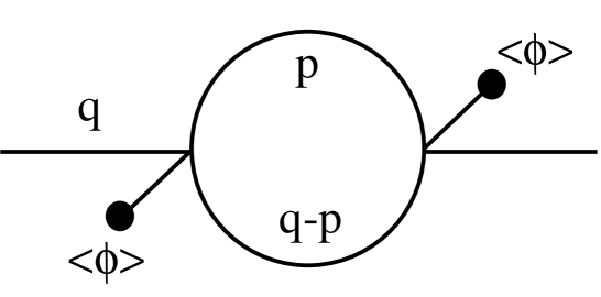
Figure 1: Diagram of the external-momentum dependent self-energy at one-loop.

$$\Pi(q_{0}^{2},{\bf q}^{2})=\frac{\lambda^{2}\bar{\phi}^{2}}{2}\int_{p}\frac{1}{p_{0}^{2}+{\bf p}^{2}+M^{2}+\frac{\lambda\bar{\phi}^{2}}{2}}\frac{1}{(q_{0}-p_{0})^{2}+({\bf q-p})^{2}+M^{2}+\frac{\lambda\bar{\phi}^{2}}{2}}.$$ (15)

The initial conditions of $K_{0}(\bar{\phi};M^{2})$ and $K_{s}(\bar{\phi};M^{2})$ are given by the coefficients of $-q_{0}^{2}$ and $-{\bf q}^{2}$ respectively. We, therefore, get

$$K_{0}(\bar{\phi};M^{2}) = 1-\left.\frac{d\Pi(q_{0}^{2},{\bf q}^{2})}{dq_{0}^{2}}\right|_{q_{i}=0,q_{0}=0}$$

$$= 1-\frac{\lambda^{2}\bar{\phi}^{2}}{2}\int_{p}\left[\frac{1}{(p_{0}^{2}+{\bf p}^{2}+M^{2}+\frac{\lambda\bar{\phi}^{2}}{2})^{3}}-\frac{M^{2}+\frac{\lambda\bar{\phi}^{2}}{2}}{(p_{0}^{2}+{\bf p}^{2}+M^{2}+\frac{\lambda\bar{\phi}^{2}}{2})^{4}}\right],$$

$$K_{s}(\bar{\phi};M^{2}) = 1-\left.\frac{d\Pi(q_{0}^{2},{\bf q}^{2})}{d{\bf q}^{2}}\right|_{q_{0}=0,q_{i}=0}$$

$$= 1+\frac{\lambda\bar{\phi}^{2}}{6}\int_{p}\frac{1}{(p_{0}^{2}+{\bf p}^{2}+M^{2}+\frac{\lambda^{2}\bar{\phi}^{2}}{2})^{3}}.$$

We have calculated the evolution equation in §2.1 and the initial condition in §2.2. Since some of them, e.g.. the one-loop effective potential, has an ultraviolet divergence, we have to renormalize it by the counter terms. Instead of considering this contribution, we simply assume that the renormalization effect is small and discard it. The contribution is, actually, small comparing with the finite temperature contribution around a critical temperature in most cases. We thus need to deal with only the temperature dependent pieces in the integrals of $\frac{\partial\Gamma}{\partial m^{2}}$ and the initial condition. To do so, we only perform the following replacement in Eq.(11),(2.1),(2.1),(14),(2.2) ,(2.2),

$$\int_{p}\ \ \ \ \ \hbox{with}\ \ \ \ \ 2\int\frac{d^{4}p}{(2\pi)^{4}i}\frac{1}{\exp(p_{0}/T)-1}.$$

We note that under the local potential approximation that $K_{0}=K_{s}=1$, the evolution equation of the effective potential reproduce our previous equation.[28, 29].

3 Results and Summary

We solved the simultaneous evolution equation Eq.(11), Eq.(2.1) and Eq.(2.1) with the initial condition Eq.(14), Eq.(2.2) and Eq.(2.2) numerically. We used an extended Crank-Nicholson method, which is explained in the appendix of Ref[29], to solve the partial differential equation. We could solve the equation at most temperatures above the critical one. Unfortunately, we can not, however, solve the equation at temperatures very close to the critical one due to numerical problems. We tried several improvements of the numerical method but failed. We, therefore, show only obtained results in the present paper. This equation may be solved at arbitrary temperature if excellent numerical methods to solve a partial differential equation are invented. Or ability of computers progresses highly so that we can calculate with much higher precision. We use a mass unit, $\mu=1$

We show the effective potential above the critical temperature in Fig.2 for $\lambda=1$. We observe behavior of a second order phase transition up to this temperature. This effective potential seems to be cone-shaped. The critical temperature is estimated to be lower than that of the local potential approximation by $2\%$.

We show $K_{0}$ and $K_{s}$ in Fig.3 for $\lambda=1$. They are very similar in spite of the violation of the Lorenz invariance in this case while the initial condition is quite different.

In summary, we derived an evolution equation of the effective action with respect to the mass squared in the $Z_{2}$-invariant scalar theory. We then approximated the effective action by the derivative expansion. We showed that the previous evolution equation of the effective potential can be derived as the leading approximation, the local potential approximation. We next derived the evolution equation of the next-to-leading approximation which is the simultaneous partial differential equation. We finally solved the equation numerically. Though we could solve it at most temperatures above the critical one, we could not do it under a certain temperature very close to the critical one unfortunately. However, this equation may be solved at arbitrary temperatures if excellent numerical methods to solve a partial differential equation are invented or ability of computers progresses highly. Anyway, we constructed the systematic method to improve the auxiliary mass method in principle.

We are suported by JSPS.

\begin{picture}(8.0,4.0)\centerline{\hbox{ \epsfbox{epot.EPSF} }} \end{picture}

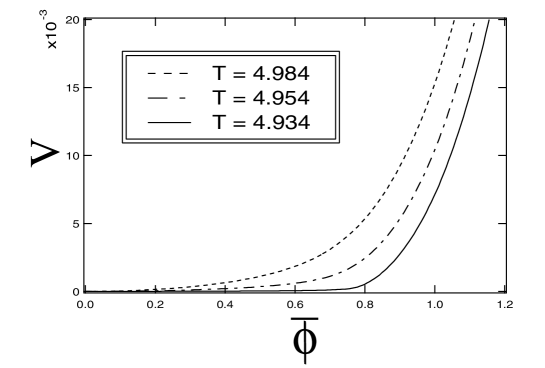
Figure 2: Effective potential around the critical temperature ($\lambda=1$).

\begin{picture}(8.0,8.0)\centerline{\hbox{ \epsfbox{kcom.EPSF} }} \end{picture}

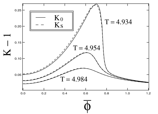
Figure 3: The coefficient functions of the second derivative terms in the effective action, $K_{0}$ and $K_{s}$ ($\lambda=1$).

Appendix

In this appendix, we show the derivation of ${\partial\Gamma}/{\partial m^{2}}$ in detail. Some notations are given in the chapter 2. The effective action $\Gamma[\phi_{c}]$ for the Lagrangian Eq.(1) is defined as usual,

$$\Gamma[\phi_{c}] \equiv W[J_{m}]-\int d^{4}xJ_{m}(x)\phi_{c}(x),$$ (18)

$$W[J_{m}] \equiv \log(Z[J_{m}]),$$

$$Z[J_{m}] \equiv \int{\cal D}[\phi]\exp\left(\int d^{4}x{\cal L}_{E}\right).$$

The equation(2.1) is, then, derived as follows,

$$\frac{\partial\Gamma[\phi_{c}]}{\partial m^{2}} = \frac{1}{Z[J_{m}]}\int{\cal D}[\phi]\left[\int\left\{d^{4}x\frac{1}{2}(-\phi(x)^{2})+\frac{\partial J_{m}(x)}{\partial m^{2}}\phi(x)\right\}\exp\left\{\int d^{4}x{\cal L}_{E}\right\}\right]$$ (19)

$$-\int d^{4}x\frac{\partial J_{m}(x)}{\partial m^{2}}\phi_{c}(x)$$

$$= -\frac{1}{2}\int d^{4}x<\phi(x)^{2}>$$

$$= -\frac{1}{2}\int d^{4}x\ \phi_{c}(x)^{2}-\frac{1}{2}\int d^{4}x(M)_{xx}^{-1}.$$

Since Eq.(2.1) is a functional equation, it can not be solved directly. We, therefore, limit functional space and expand $\Gamma[\phi_{c}]$ in powers of derivatives[33, 34], (see Eq.(5))

$$\Gamma[\phi_{c}]=\int d^{4}x\left[-V(\phi_{c}^{2})-\frac{1}{2}K_{0}(\phi_{c}^{2})(\partial_{0}\phi_{c})^{2}-\frac{1}{2}K_{s}(\phi_{c}^{2})(\nabla\phi_{c})^{2}+\cdots\right],$$

where “$\cdots$” denotes terms with higher derivative which are omitted here and equating the coefficient functionals of $(\partial\phi_{c})$ in the both side of Eq.(2.1).

The left hand side of Eq.(19) is calculated to be Eq.(6) by simply differentiating $\Gamma$ with respect to $m^{2}$,

$$-\frac{\partial\Gamma}{\partial m^{2}}=\int d^{4}x\left[\frac{\partial V}{\partial m^{2}}+\frac{1}{2}\frac{\partial K_{0}}{\partial m^{2}}(\partial_{0}\phi_{c})^{2}+\frac{1}{2}\frac{\partial K_{s}}{\partial m^{2}}(\nabla\phi_{c})^{2}\right].$$

It is very complicated to calculate r.h.s. of Eq.(19). First we calculate $M_{yx}$. The derivative of the effective action $\Gamma[\phi_{c}]$ with respect to $\phi_{c}(x)$ is,

$$\frac{\delta\Gamma[\phi_{c}]}{\delta\phi_{c}(x)}= - V^{{}^{\prime}}(\phi_{c}(x))$$

$$+\frac{1}{2}K_{0}^{{}^{\prime}}(\phi_{c}(x))(\partial_{0}\phi_{c}(x))^{2}+K_{0}(\phi_{c}(x))(\partial_{0}^{2}\phi_{c}(x))$$

$$+\left\{K_{0}\leftrightarrow K_{s},\partial_{0}\leftrightarrow\nabla\right\}.$$

Here, we assume that we can make a partial integral freely without a surface term.

We define the operator $M_{xy}$ in the following sense. An operator $O_{xy}$ defined through functional derivative with respect to $\phi(x)$, say $\delta F(\phi(y))/\delta\phi(x)$, acts on any appropriate test function, say $T(y)$,

$$OT(x) \equiv \int d^{4}y\left\{\frac{\delta}{\delta\phi(x)}F(\phi(y))\right\}T(y).$$

In particular, if $F(\phi(y))$ contains the derivative of $\phi(y)$, say $F(\phi(y))=G(\phi(y))\partial\phi(y)$,

$$OT(x) \equiv \int d^{4}y\left\{\frac{\delta}{\delta\phi(x)}G(\phi(y))\partial\phi(y)\right\}T(y).$$ (21)

$$\equiv \int d^{4}y\delta(y-x)\left[G^{{}^{\prime}}(\phi(y))\partial\phi(y)T(y)-\partial\left\{G(\phi(y))T(y)\right\}\right].$$

In order to obtain Eq.(2.1) and to determine the inverse of $M_{yx}$ around $\bar{\phi}$, we divide the Eq.(2.1) into two pieces (Eq.(9)),

$$M_{yx} = A_{yx}-B_{yx},$$

$$A_{yx} = \delta(y-x)(-\overline{K}_{0}\partial_{0}^{2}-\overline{K}_{s}\nabla^{2}+\overline{V}^{\prime\prime}),$$

$$B_{yx} = -\delta(y-x)\left[\widetilde{V}^{{}^{\prime\prime}}(\phi_{c}(y))\right.$$

$$- \left\{\frac{1}{2}K_{0}^{{}^{\prime\prime}}(\phi_{c}(y))(\partial_{0}\phi_{c}(y))^{2}+K_{0}^{{}^{\prime}}(\phi_{c}(y))\partial_{0}\phi_{c}(y)\partial_{y_{0}}\right.$$

$$+ \left.K_{0}^{{}^{\prime}}(\phi_{c}(y))\partial_{0}^{2}\phi_{c}(y)+\widetilde{K}_{0}(\phi_{c}(y))\partial_{y_{0}}^{2}\right\}$$

$$-\left.\left\{K_{0}\leftrightarrow K_{s},\partial_{y_{0}}\leftrightarrow\nabla_{y}\right\}\right].$$

The inverse of $M_{yx}$ is, then, expanded as,

$$(M^{-1})_{xy} = \{(A^{-1})(\sum_{n=0}^{n=\infty}(BA^{-1})^{n})\}_{xy}.$$ (22)

Here, the multiplication of the ”matrix” $A$ and $B$ is taken in the following sense,

$$(AB)_{xy}=\int d^{4}zA_{xz}B_{zy}.$$

The inverse of $A_{xy}$ is calculated easily,

$$(A^{-1})_{xy}=\int_{p}\frac{1}{\nu_{p}}\exp\left\{ip(x-y)\right\},$$ (23)

where $\nu_{p}=\overline{K}_{0}p_{0}^{2}+\overline{K}_{s}{\bf p}^{2}+\overline{V}^{\prime\prime}$.

We need terms with $(\partial\phi_{c})^{n}(n=0,2)$ to evaluate r.h.s of Eq.(19). Such terms are contained only in the first three terms in Eq.(22),

$$(M^{-1})_{xy} = (A^{-1})_{xy}$$

$$+(A^{-1}BA^{-1})_{xy}$$

$$+(A^{-1}BA^{-1}BA^{-1})_{xy}.$$

The relevant terms in Eq.(19) are, therefore, the following,

$$\int d^{4}x(M^{-1})_{xx} = \int d^{4}x(A^{-1})_{xx}$$ (27)

$$+\int d^{4}x(A^{-1}BA^{-1})_{xx}$$

$$+\int d^{4}x(A^{-1}BA^{-1}BA^{-1})_{xx}.$$

We next calculate Eq.(27)-(27) up to terms with the second derivative of $\phi_{c}(x)$. From Eq.(23) the first term (27) is easy to calculate,

$$\int d^{4}x(A^{-1})_{xx}=\int d^{4}x\int_{p}\frac{1}{\nu_{p}}.$$ (28)

The second term Eq.(27) is

$$\int d^{4}x(A^{-1}BA^{-1})_{xx}$$ (29)

$$= \int d^{4}x\int d^{4}y\int d^{4}z\int_{p}\frac{1}{\nu_{p}}\exp\left\{ip(x-y)\right\}$$

$$\delta(y-z)\left[-\widetilde{V}^{{}^{\prime\prime}}(\phi_{c}(y))+\left\{\frac{1}{2}K_{0}^{{}^{\prime\prime}}(\phi_{c}(y))(\partial_{0}\phi_{c}(y))^{2}+K_{0}^{{}^{\prime}}(\phi_{c}(y))\partial_{0}\phi_{c}(y)\partial_{y_{0}}\right.\right.$$

$$\left.+\left.K_{0}^{{}^{\prime}}(\phi_{c}(y))\partial_{0}^{2}\phi_{c}(y)+\tilde{K}_{0}(\phi_{c}(y))\partial_{y_{0}}^{2}\right\}+\left\{K_{0}\leftrightarrow K_{s},\partial_{y_{0}}\leftrightarrow\nabla_{y}\right\}\right]$$

$$\int_{q}\frac{1}{\nu_{q}}\exp\left\{iq(z-x)\right\}$$

(integrating over $$z$$.)

$$= \int d^{4}x\int d^{4}y\int_{p}\int_{q}\frac{1}{\nu_{p}}\frac{1}{\nu_{q}}\exp\left\{ip(x-y)\right\}\exp\left\{iq(y-x)\right\}$$

$$\left[-\widetilde{V}^{{}^{\prime\prime}}(\phi_{c}(y))+\left\{\frac{1}{2}K_{0}^{{}^{\prime\prime}}(\phi_{c}(y))(\partial_{0}\phi_{c}(y))^{2}+K_{0}^{{}^{\prime}}(\phi_{c}(y))\partial_{0}\phi_{c}(y)iq_{0}\right.\right.$$

$$\left.+\left.K_{0}^{{}^{\prime}}(\phi_{c}(y))\partial_{0}^{2}\phi_{c}(y)-\tilde{K}_{0}(\phi_{c}(y))q_{0}^{2}\right\}+\left\{K_{0}\leftrightarrow K_{s},\partial_{0}\leftrightarrow\nabla,q_{0}\leftrightarrow{\bf q}\right\}\right]$$

(integrating over $$x q y x$$ and then replacing by .)

$$= \int d^{4}x\int_{p}\frac{1}{\nu_{p}^{2}}$$

$$\left[-\widetilde{V}^{{}^{\prime\prime}}(\phi_{c}(x))+\left\{\frac{1}{2}K^{{}^{\prime\prime}}_{0}(\phi_{c}(x))(\partial_{0}\phi(x))^{2}+K_{0}^{{}^{\prime}}(\phi_{c}(x))\partial_{0}\phi(x)ip_{0}\right.\right.$$

$$\left.+\left.K_{0}^{{}^{\prime}}(\phi_{c}(x))\partial_{0}^{2}\phi(x)-\tilde{K}_{0}(\phi_{c}(x))p_{0}^{2}\right\}+\left\{K_{0}\leftrightarrow K_{s},\partial_{0}\leftrightarrow\nabla,p_{0}\leftrightarrow{\bf p}\right\}\right]$$

(partially integrating the fourth term.)

$$= \int d^{4}x\int_{p}\frac{1}{\nu_{p}^{2}}\left[-\widetilde{V}^{{}^{\prime\prime}}(\phi_{c}(x))-\left\{\frac{1}{2}K^{{}^{\prime\prime}}_{0}(\phi_{c}(x))(\partial_{0}\phi_{c}(x))^{2}+\tilde{K}_{0}(\phi_{c}(x))p_{0}^{2}\right\}\right.$$

$$\left.-\left\{K_{0}\leftrightarrow K_{s},\partial_{0}\leftrightarrow\nabla,p_{0}\leftrightarrow{\bf p}\right\}\right].$$

$$= \int d^{4}x\int_{p}\frac{1}{\nu_{p}^{2}}\left[-\left\{\frac{1}{2}\overline{K}_{0}^{\prime\prime}(\partial_{0}\phi_{c})^{2}+\frac{1}{2}\overline{K}_{s}^{\prime\prime}(\nabla\phi_{c})^{2}\right\}\right]$$

$$+(terms\ which\ vanish\ at\ \phi_{c}(x)=\bar{\phi}\ like\ \widetilde{V}^{\prime\prime}\times(something)).$$

Since we set $\phi_{c}(x)=\bar{\phi}$ after the matching of Eq.(2.1), we have no contribution to the evolution equation from the terms which vanish at $\phi_{c}(x)=\bar{\phi}$. We thus leave only terms which remain finite at $\phi_{c}(x)=\bar{\phi}$ from now on. The third term (27) is very complicated to evaluate,

$$\int d^{4}x(A^{-1}BA^{-1}BA^{-1})_{xx}$$

$$= \int d^{4}x\int d^{4}y\int d^{4}z\int d^{4}u\int d^{4}v\int_{p}\frac{1}{\nu_{p}}\exp\left\{ip(x-y)\right\}$$

$$\delta(y-z)\left[-\widetilde{V}^{{}^{\prime\prime}}(\phi_{c}(y))+\left\{\frac{1}{2}K_{0}^{{}^{\prime\prime}}(\phi_{c}(y))(\partial_{0}\phi_{c}(y))^{2}+K_{0}^{{}^{\prime}}(\phi_{c}(y))\partial_{0}\phi_{c}(y)\partial_{y_{0}}\right.\right.$$

$$\left.+\left.K_{0}^{{}^{\prime}}(\phi_{c}(y))\partial_{0}^{2}\phi_{c}(y)+\tilde{K}_{0}(\phi_{c}(y))\partial_{y_{0}}^{2}\right\}+\left\{K_{0}\leftrightarrow K_{s},\partial_{y_{0}}\leftrightarrow\nabla_{y}\right\}\right]$$

$$\int_{q}\frac{1}{\nu_{q}}\exp\left\{iq(z-u)\right\}$$

$$\delta(u-v)\left[-\widetilde{V}^{{}^{\prime\prime}}(\phi_{c}(u))+\left\{\frac{1}{2}K_{0}^{{}^{\prime\prime}}(\phi_{c}(u))(\partial_{0}\phi_{c}(u))^{2}+K_{0}^{{}^{\prime}}(\phi_{c}(u))\partial_{0}\phi_{c}(u)\partial_{u_{0}}\right.\right.$$

$$\left.+\left.K_{0}^{{}^{\prime}}(\phi_{c}(u))\partial_{0}^{2}\phi_{c}(u)+\tilde{K}_{0}(\phi_{c}(u))\partial_{u_{0}}^{2}\right\}+\left\{K_{0}\leftrightarrow K_{s},\partial_{u_{0}}\leftrightarrow\nabla_{u}\right\}\right]$$

$$\int_{r}\frac{1}{\nu_{r}}\exp\left\{ir(v-x)\right\}$$

(integrating over $$x,z,v,r u x$$ and replacing with )

$$= \int d^{4}x\int d^{4}y\int_{p}\int_{q}\frac{1}{\nu_{p}^{2}}\frac{1}{\nu_{q}}\exp\left\{i(p-q)(x-y)\right\}$$

$$\left[-\widetilde{V}^{{}^{\prime\prime}}(\phi_{c}(x))+\left\{\frac{1}{2}K^{{}^{\prime\prime}}_{0}(\phi_{c}(x))(\partial_{0}\phi_{c}(x))^{2}+K_{0}^{{}^{\prime}}(\phi_{c}(x))\partial_{0}\phi_{c}(x)ip_{0}\right.\right.$$

$$\left.+\left.K_{0}^{{}^{\prime}}(\phi_{c}(x))\partial_{0}^{2}\phi_{c}(x)-\tilde{K}_{0}(\phi_{c}(x))p_{0}^{2}\right\}+\left\{K_{0}\leftrightarrow K_{s},\partial_{0}\leftrightarrow\nabla,p_{0}\leftrightarrow{\bf p}\right\}\right]$$

$$\times \left[-\widetilde{V}^{{}^{\prime\prime}}(\phi_{c}(y))+\left\{\frac{1}{2}K_{0}^{{}^{\prime\prime}}(\phi_{c}(y))(\partial_{0}\phi_{c}(y))^{2}+K_{0}^{{}^{\prime}}(\phi_{c}(y))\partial_{0}\phi_{c}(y)iq_{0}\right.\right.$$

$$\left.+\left.K_{0}^{{}^{\prime}}(\phi_{c}(y))\partial_{0}^{2}\phi_{c}(y)-\tilde{K}_{0}(\phi_{c}(y))q_{0}^{2}\right\}+\left\{K_{0}\leftrightarrow K_{s},\partial_{0}\leftrightarrow\nabla,q_{0}\leftrightarrow{\bf q}\right\}\right].$$

(partially integrating the term with $$\partial_{0}^{2}\phi$$.)

$$= \int d^{4}x\int d^{4}y\int_{p}\int_{q}\frac{1}{\nu_{p}^{2}}\frac{1}{\nu_{q}}\exp\left\{i(p-q)(x-y)\right\}$$

$$\left[-\widetilde{V}^{{}^{\prime\prime}}(\phi_{c}(x))+\left\{-\frac{1}{2}K^{{}^{\prime\prime}}_{0}(\phi_{c}(x))(\partial_{0}\phi_{c}(x))^{2}+K_{0}^{{}^{\prime}}(\phi_{c}(x))\partial_{0}\phi_{c}(x)iq_{0}\right.\right.$$

$$\left.-\left.\tilde{K}_{0}(\phi_{c}(x))p_{0}^{2}\right\}+\left\{K_{0}\leftrightarrow K_{s},\partial_{0}\leftrightarrow\nabla,p_{0}\leftrightarrow{\bf p},q_{0}\leftrightarrow{\bf q}\right\}\right]$$

$$\times \left[-\widetilde{V}^{{}^{\prime\prime}}(\phi_{c}(y))+\left\{-\frac{1}{2}K_{0}^{{}^{\prime\prime}}(\phi_{c}(y))(\partial_{0}\phi_{c}(y))^{2}+K_{0}^{{}^{\prime}}(\phi_{c}(y))\partial_{0}\phi_{c}(y)ip_{0}\right.\right.$$

$$\left.-\left.\tilde{K}_{0}(\phi_{c}(y))q_{0}^{2}\right\}+\left\{K_{0}\leftrightarrow K_{s},\partial_{0}\leftrightarrow\nabla,p_{0}\leftrightarrow{\bf p},q_{0}\leftrightarrow{\bf q}\right\}\right].$$

By the following variable exchange,

$$\left\{\begin{array}[]{lll}p&\longrightarrow&p+q\\ q&\longrightarrow&p\end{array}\right.,$$ (32)

we obtain,

$$= \int d^{4}x\int d^{4}y\int_{p}\int_{q}\frac{1}{\nu_{p+q}^{2}}\frac{1}{\nu_{p}}\exp\left\{iq(x-y)\right\}$$

$$\left[-\widetilde{V}^{{}^{\prime\prime}}(\phi_{c}(x))+\left\{-\frac{1}{2}K^{{}^{\prime\prime}}_{0}(\phi_{c}(x))(\partial_{0}\phi_{c}(x))^{2}+K_{0}^{{}^{\prime}}(\phi_{c}(x))\partial_{0}\phi_{c}(x)ip_{0}\right.\right.$$

$$\left.-\left.\tilde{K}_{0}(\phi_{c}(x))(p+q)_{0}^{2}\right\}+\left\{K_{0}\leftrightarrow K_{s},\partial_{0}\leftrightarrow\nabla,p_{0}\leftrightarrow{\bf p},q_{0}\leftrightarrow{\bf q}\right\}\right]$$

$$\times \left[-\widetilde{V}^{{}^{\prime\prime}}(\phi_{c}(y))+\left\{-\frac{1}{2}K_{0}^{{}^{\prime\prime}}(\phi_{c}(y))(\partial_{0}\phi_{c}(y))^{2}+K_{0}^{{}^{\prime}}(\phi_{c}(y))\partial_{0}\phi_{c}(y)i(p+q)_{0}\right.\right.$$

$$\left.-\left.\tilde{K}_{0}(\phi_{c}(y))p_{0}^{2}\right\}+\left\{K_{0}\leftrightarrow K_{s},\partial_{0}\leftrightarrow\nabla,p_{0}\leftrightarrow{\bf p},q_{0}\leftrightarrow{\bf q}\right\}\right].$$

$$= \int d^{4}x\int d^{4}y\int_{p}\int_{q}\frac{\exp\left\{iq(x-y)\right\}}{\nu_{p}^{3}}$$

$$\left\{1-\frac{\left\{\overline{K}_{0}(4p_{0}q_{0}+2q_{0}^{2})+\overline{K}_{s}(4{\bf pq}+2{\bf q^{2}}\right\}}{\nu_{p}}+\frac{12\left\{\overline{K}_{0}p_{0}q_{0}+\overline{K}_{s}{\bf pq}\right\}^{2}}{\nu_{p}^{2}}+\cdots\right\}$$

$$\left[-\widetilde{V}^{{}^{\prime\prime}}(\phi_{c}(x))+\left\{-\frac{1}{2}K^{{}^{\prime\prime}}_{0}(\phi_{c}(x))(\partial_{0}\phi_{c}(x))^{2}+K_{0}^{{}^{\prime}}(\phi_{c}(x))\partial_{0}\phi_{c}(x)ip_{0}\right.\right.$$

$$\left.-\left.\tilde{K}_{0}(\phi_{c}(x))(p+q)_{0}^{2}\right\}+\left\{K_{0}\leftrightarrow K_{s},\partial_{0}\leftrightarrow\nabla,p_{0}\leftrightarrow{\bf p},q_{0}\leftrightarrow{\bf q}\right\}\right]$$

$$\times \left[-\widetilde{V}^{{}^{\prime\prime}}(\phi_{c}(y))+\left\{-\frac{1}{2}K_{0}^{{}^{\prime\prime}}(\phi_{c}(y))(\partial_{0}\phi_{c}(y))^{2}+K_{0}^{{}^{\prime}}(\phi_{c}(y))\partial_{0}\phi_{c}(y)i(p+q)_{0}\right.\right.$$

$$\left.-\left.\tilde{K}_{0}(\phi_{c}(y))p_{0}^{2}\right\}+\left\{K_{0}\leftrightarrow K_{s},\partial_{0}\leftrightarrow\nabla,p_{0}\leftrightarrow{\bf p},q_{0}\leftrightarrow{\bf q}\right\}\right],$$

where we take the terms up to $q^{2}$ since we will replace $q$ to the derivative and need terms with second derivatives. Similarly, by the following exchange of the variables,

$$\left\{\begin{array}[]{lll}p&\longrightarrow&p\\ q&\longrightarrow&p+q\end{array}\right.,$$ (35)

we have,

$$= \int d^{4}x\int d^{4}y\int_{p}\int_{q}\frac{1}{\nu_{p+q}}\frac{1}{\nu_{p}^{2}}\exp\left\{iq(x-y)\right\}$$

$$\left[-\widetilde{V}^{{}^{\prime\prime}}(\phi_{c}(x))+\left\{-\frac{1}{2}K^{{}^{\prime\prime}}_{0}(\phi_{c}(x))(\partial_{0}\phi_{c}(x))^{2}+K_{0}^{{}^{\prime}}(\phi_{c}(x))\partial_{0}\phi_{c}(x)ip_{0}\right.\right.$$

$$\left.-\left.\tilde{K}_{0}(\phi_{c}(x))(p+q)_{0}^{2}\right\}+\left\{K_{0}\leftrightarrow K_{s},\partial_{0}\leftrightarrow\nabla,p_{0}\leftrightarrow{\bf p},q_{0}\leftrightarrow{\bf q}\right\}\right]$$

$$\times \left[-\widetilde{V}^{{}^{\prime\prime}}(\phi_{c}(y))+\left\{-\frac{1}{2}K_{0}^{{}^{\prime\prime}}(\phi_{c}(y))(\partial_{0}\phi_{c}(y))^{2}+K_{0}^{{}^{\prime}}(\phi_{c}(y))\partial_{0}\phi_{c}(y)i(p+q)_{0}\right.\right.$$

$$\left.-\left.\tilde{K}_{0}(\phi_{c}(y))p_{0}^{2}\right\}+\left\{K_{0}\leftrightarrow K_{s},\partial_{0}\leftrightarrow\nabla,p_{0}\leftrightarrow{\bf p},q_{0}\leftrightarrow{\bf q}\right\}\right].$$

$$= \int d^{4}x\int d^{4}y\int_{p}\int_{q}\frac{\exp\left\{iq(x-y)\right\}}{\nu_{p}^{3}}$$

$$\left\{1-\frac{\left\{\overline{K}_{0}(2p_{0}q_{0}+q_{0}^{2})+\overline{K}_{s}(2{\bf pq}+{\bf q^{2}})\right\}}{\nu_{p}}+\frac{4\left\{\overline{K}_{0}p_{0}q_{0}+\overline{K}_{s}{\bf pq}\right\}^{2}}{\nu_{p}^{2}}+\cdots\right\}$$

$$\left[-\widetilde{V}^{{}^{\prime\prime}}(\phi_{c}(x))+\left\{-\frac{1}{2}K^{{}^{\prime\prime}}_{0}(\phi_{c}(x))(\partial_{0}\phi_{c}(x))^{2}+K_{0}^{{}^{\prime}}(\phi_{c}(x))\partial_{0}\phi_{c}(x)ip_{0}\right.\right.$$

$$\left.-\left.\tilde{K}_{0}(\phi_{c}(x))(p+q)_{0}^{2}\right\}+\left\{K_{0}\leftrightarrow K_{s},\partial_{0}\leftrightarrow\nabla,p_{0}\leftrightarrow{\bf p},q_{0}\leftrightarrow{\bf q}\right\}\right]$$

$$\times \left[-\widetilde{V}^{{}^{\prime\prime}}(\phi_{c}(y))+\left\{-\frac{1}{2}K_{0}^{{}^{\prime\prime}}(\phi_{c}(y))(\partial_{0}\phi_{c}(y))^{2}+K_{0}^{{}^{\prime}}(\phi_{c}(y))\partial_{0}\phi_{c}(y)i(p+q)_{0}\right.\right.$$

$$\left.-\left.\tilde{K}_{0}(\phi_{c}(y))p_{0}^{2}\right\}+\left\{K_{0}\leftrightarrow K_{s},\partial_{0}\leftrightarrow\nabla,p_{0}\leftrightarrow{\bf p},q_{0}\leftrightarrow{\bf q}\right\}\right].$$

By comparing Eq.(3) with Eq.(3), we have the following ”identity”,

$$0 = \int d^{4}x\int d^{4}y\int_{p}\int_{q}\frac{\exp\left\{iq(x-y)\right\}}{\nu_{p}^{3}}$$

$$\left\{-\frac{\left\{\overline{K}_{0}(2p_{0}q_{0}+q_{0}^{2})+\overline{K}_{s}(2{\bf pq}+{\bf q^{2}})\right\}}{\nu_{p}}+\frac{8\left\{\overline{K}_{0}p_{0}q_{0}+\overline{K}_{s}{\bf pq}\right\}^{2}}{\nu_{p}^{2}}+\cdots\right\}$$

$$\left[-\widetilde{V}^{{}^{\prime\prime}}(\phi_{c}(x))+\left\{-\frac{1}{2}K^{{}^{\prime\prime}}_{0}(\phi_{c}(x))(\partial_{0}\phi_{c}(x))^{2}+K_{0}^{{}^{\prime}}(\phi_{c}(x))\partial_{0}\phi_{c}(x)ip_{0}\right.\right.$$

$$\left.-\left.\tilde{K}_{0}(\phi_{c}(x))(p+q)_{0}^{2}\right\}+\left\{K_{0}\leftrightarrow K_{s},\partial_{0}\leftrightarrow\nabla,p_{0}\leftrightarrow{\bf p},q_{0}\leftrightarrow{\bf q}\right\}\right]$$

$$\times \left[-\widetilde{V}^{{}^{\prime\prime}}(\phi_{c}(y))+\left\{-\frac{1}{2}K_{0}^{{}^{\prime\prime}}(\phi_{c}(y))(\partial_{0}\phi_{c}(y))^{2}+K_{0}^{{}^{\prime}}(\phi_{c}(y))\partial_{0}\phi_{c}(y)i(p+q)_{0}\right.\right.$$

$$\left.-\left.\tilde{K}_{0}(\phi_{c}(y))p_{0}^{2}\right\}+\left\{K_{0}\leftrightarrow K_{s},\partial_{0}\leftrightarrow\nabla,p_{0}\leftrightarrow{\bf p},q_{0}\leftrightarrow{\bf q}\right\}\right].$$

Indeed, this identity holds exactly for the coefficient functions of $(\nabla\phi_{c})^{2}$, though it is not the case for that of $(\partial_{0}\phi_{c})^{2}$. Anyway, we use this identity and rewrite (or define) the third term (27) in the following,

$$\int d^{4}x(A^{-1}BA^{-1}BA^{-1})_{xx}$$

$$= \int d^{4}x\int d^{4}y\int_{p}\int_{q}\frac{\exp\left\{iq(x-y)\right\}}{\nu_{p}^{3}}$$

$$\left\{1-\frac{1}{2}\frac{\left\{\overline{K}_{0}(2p_{0}q_{0}+q_{0}^{2})+\overline{K}_{s}(2{\bf pq}+{\bf q^{2}})\right\}}{\nu_{p}}+\cdots\right\}$$

$$\left[-\widetilde{V}^{{}^{\prime\prime}}(\phi_{c}(x))+\left\{-\frac{1}{2}K^{{}^{\prime\prime}}_{0}(\phi_{c}(x))(\partial_{0}\phi_{c}(x))^{2}+K_{0}^{{}^{\prime}}(\phi_{c}(x))\partial_{0}\phi_{c}(x)ip_{0}\right.\right.$$

$$\left.-\left.\tilde{K}_{0}(\phi_{c}(x))(p+q)_{0}^{2}\right\}+\left\{K_{0}\leftrightarrow K_{s},\partial_{0}\leftrightarrow\nabla,p_{0}\leftrightarrow{\bf p},q_{0}\leftrightarrow{\bf q}\right\}\right]$$

$$\times \left[-\widetilde{V}^{{}^{\prime\prime}}(\phi_{c}(y))+\left\{-\frac{1}{2}K_{0}^{{}^{\prime\prime}}(\phi_{c}(y))(\partial_{0}\phi_{c}(y))^{2}+K_{0}^{{}^{\prime}}(\phi_{c}(y))\partial_{0}\phi_{c}(y)i(p+q)_{0}\right.\right.$$

$$\left.-\left.\tilde{K}_{0}(\phi_{c}(y))p_{0}^{2}\right\}+\left\{K_{0}\leftrightarrow K_{s},\partial_{0}\leftrightarrow\nabla,p_{0}\leftrightarrow{\bf p},q_{0}\leftrightarrow{\bf q}\right\}\right].$$

Note that there is no contribution from Eq.(3) to the evolution equation for the effective potential $V$ since the constant terms always include $\tilde{K}$ and $\tilde{V}^{\prime\prime}$ which are zero at $\phi_{c}(x)=\bar{\phi}$ by definition.

From now on we evaluate the coefficient functions of $(\partial\phi_{c}(x))^{2}$. First we calculate the first term of Eq.(3). There are three contributions from this term,

$$\int d^{4}x\int d^{4}y\int_{p}\int_{q}\frac{\exp\left\{iq(x-y)\right\}}{\nu_{p}^{3}}$$ (39)

$$\left\{K_{0}^{{}^{\prime}}(\phi_{c}(x))\partial_{0}\phi_{c}(x)ip_{0}+K_{s}^{{}^{\prime}}(\phi_{c}(x))\nabla\phi_{c}(x)i{\bf p}\right\}$$

$$\times \left\{K_{0}^{{}^{\prime}}(\phi_{c}(y))\partial_{0}\phi_{c}(y)ip_{0}+K_{s}^{{}^{\prime}}(\phi_{c}(y))\nabla\phi_{c}(y)i{\bf p}\right\}$$

(integrating over $$q y$$ and .)

$$= \int d^{4}x\int_{p}\frac{-1}{\nu_{p}^{3}}\left\{\overline{K}_{0}^{\prime}(\partial_{0}\phi_{c})p_{0}+\overline{K}_{s}^{\prime}(\nabla\phi_{c}){\bf p}\right\}^{2},$$

$$\int d^{4}x\int d^{4}y\int_{p}\int_{q}\frac{\exp\left\{iq(x-y)\right\}}{\nu_{p}^{3}}$$

$$\left[\left\{K_{0}^{{}^{\prime}}(\phi_{c}(x))\partial_{0}\phi_{c}(x)iq_{0}+K_{s}^{{}^{\prime}}(\phi_{c}(x))\nabla\phi_{c}(x)i{\bf q}\right\}\times\right.$$

$$\hskip 28.45274pt\left.\left\{-\tilde{K}_{0}(\phi_{c}(y))p_{0}^{2}-\tilde{K}_{s}(\phi_{c}(y)){\bf p}^{2}-V^{\prime\prime}(\phi_{c}(y))\right\}\right.$$

$$+\left.2\left\{K_{0}^{{}^{\prime}}(\phi_{c}(x))\partial_{0}\phi_{c}(x)ip_{0}+K_{s}^{{}^{\prime}}(\phi_{c}(x))\nabla\phi_{c}(x)i{\bf p}\right\}\times\right.$$

$$\hskip 28.45274pt\left.\left\{-\tilde{K}_{0}(\phi_{c}(y))p_{0}q_{0}-\tilde{K}_{s}(\phi_{c}(y)){\bf pq}\right\}\right]$$

$$= \int d^{4}x\int d^{4}y\int_{p}\int_{q}\frac{1}{\nu_{p}^{3}}$$

$$\left[\left\{K_{0}^{{}^{\prime}}(\phi_{c}(x))\partial_{0}\phi_{c}(x)\partial_{x_{0}}+K_{s}^{{}^{\prime}}(\phi_{c}(x))\nabla\phi_{c}(x)\nabla_{x}\right\}\times\right.$$

$$\hskip 28.45274pt\left.\left\{-\tilde{K}_{0}(\phi_{c}(y))p_{0}^{2}-\tilde{K}_{s}(\phi_{c}(y)){\bf p}^{2}-V^{\prime\prime}(\phi_{c}(y)\right\}\right.$$

$$+\left.2\left\{K_{0}^{{}^{\prime}}(\phi_{c}(x))\partial_{0}\phi_{c}(x)ip_{0}+K_{s}^{{}^{\prime}}(\phi_{c}(x))\nabla\phi_{c}(x)i{\bf p}\right\}\times\right.$$

$$\hskip 28.45274pt\left.\left\{\tilde{K}_{0}(\phi_{c}(y))ip_{0}\partial_{x_{0}}+\tilde{K}_{s}(\phi_{c}(y))i{\bf p}\nabla_{x}\right\}\right]$$

$$\times \exp\left\{iq(x-y)\right\}$$

(partially integrating over x and then integrating over $$q y$$ and .)

$$= \int d^{4}x\int_{p}\frac{1}{\nu_{p}^{3}}\left[\left\{\overline{K}_{0}^{\prime}(\partial_{0}\phi_{c})^{2}+\overline{K}_{s}^{\prime}(\nabla\phi_{c})^{2}\right\}\left\{\overline{K}_{0}^{\prime}p_{0}^{2}+\overline{K}_{s}^{\prime}{\bf p}^{2}+\overline{V}^{\prime\prime\prime}\right\}\right.$$

$$\left.+2\left\{\overline{K}_{0}^{\prime}(\partial_{0}\phi_{c})p_{0}+\overline{K}_{s}^{\prime}(\nabla\phi_{c}){\bf p}\right\}^{2}\right],$$

and

$$\int d^{4}x\int d^{4}y\int_{p}\int_{q}\frac{\exp\left\{iq(x-y)\right\}}{\nu_{p}^{3}}$$ (41)

$$\left[\left\{-\tilde{K}_{0}(\phi_{c}(x))q_{0}^{2}-\tilde{K}_{s}(\phi_{c}(x)){\bf q}^{2}\right\}\times\right.$$

$$\hskip 28.45274pt\left.\left\{-\tilde{K}_{0}(\phi_{c}(y))p_{0}^{2}-\tilde{K}_{s}(\phi_{c}(y)){\bf p}^{2}-V^{\prime\prime}(\phi_{c}(y))\right\}\right]$$

$$= \int d^{4}x\int_{p}\frac{1}{\nu_{p}^{3}}\left\{\overline{K}_{0}^{\prime}(\partial_{0}\phi_{c})^{2}+\overline{K}_{s}^{\prime}(\nabla\phi_{c})^{2}\right\}\left\{\overline{K}_{0}^{\prime}p_{0}^{2}+\overline{K}_{s}^{\prime}{\bf p}^{2}+\overline{V}^{\prime\prime\prime}\right\}.$$

As a whole, we have the following contribution from the first term of Eq.(3),

$$\int d^{4}x\int_{p}\frac{1}{\nu_{p}^{3}}\left[2\left\{\overline{K}_{0}^{\prime}(\partial_{0}\phi_{c})^{2}+\overline{K}_{s}^{\prime}(\nabla\phi_{c})^{2}\right\}\nu_{p}^{\prime}\right.$$ (42)

$$\left.+\left\{\overline{K}_{0}^{\prime}\partial_{0}\phi_{c}p_{0}+\overline{K}_{s}^{\prime}\nabla\phi_{c}{\bf p}\right\}^{2}\right].$$

Similarly, we have the following contribution from the second term of Eq.(3),

$$\int d^{4}x\int_{p}\frac{1}{\nu_{p}^{4}}\left[-\frac{1}{2}\left\{\overline{K}_{0}^{\prime}p_{0}^{2}+\overline{K}_{s}^{\prime}{\bf p}^{2}+\overline{V}^{\prime\prime\prime}\right\}^{2}+\left\{\overline{K}_{0}(\partial_{0}\phi_{c})^{2}+\overline{K}_{s}(\nabla\phi_{c})^{2}\right\}\right.$$

$$\left.-2\left\{\overline{K}_{0}^{\prime}(\partial_{0}\phi_{c})p_{0}+\overline{K}_{s}^{\prime}(\nabla\phi_{c}){\bf p}\right\}\left\{\overline{K}_{0}(\partial_{0}\phi_{c})p_{0}+\overline{K}_{s}(\nabla\phi_{c}){\bf p}\right\}\nu^{\prime}_{p}\right].$$ (43)

Combining Eq.(28), Eq.(29), Eq.(42) and Eq.(43), we obtain the evolution equation, Eq.(2.1).