Abstract

We investigate a new “renormalization invariant analytic formulation” of calculations in quantum chromodynamics, where the renormalization group summation is correlated with the analyticity with respect to the square of the transferred momentum $Q^{2}$. The expressions for the invariant charge and matrix elements are then modified such that the unphysical singularities of the ghost pole type do not appear at all, being by construction compensated by additional nonperturbative contributions. Using the new scheme, we show that the results of calculations for a number of physical processes are stable with respect to higher-loop effects and the choice of the renormalization prescription.

Having in mind applications of the new formulation to inelastic lepton–nucleon scattering processes, we analyze the corresponding structure functions starting from the general principles of the theory expressed by the Jost–Lehmann–Dyson integral representation. We use a nonstandard scaling variable that leads to modified moments of the structure functions possessing Källén–Lehmann analytic properties with respect to $Q^{2}$. We find the relation between these “modified analytic moments” and the operator product expansion.

                                                                                       Take care of the Principles, and the
                                                                                       Principles shall take care of you.

Scientific achievements of Nikolai Nikolaevich Bogoliubov are characterized by a unique combination of determination in solving concrete scientific problems and a high level of mathematical culture. He could find the shortest path to a physical result using most general principles of the theory.

The renormalization-invariant analytic approach to quantum chromodynamics exposed here and its most recent applications are based on the works [1, 2, 3, 4] by Bogoliubov with his closest collaborators. A characteristic feature of these investigations is their strong relation with the fundamental quantum physics principles.

1 Introduction

An intrinsic ingredient of modern quantum field theory (QFT) is the renormalization group (RG) method proposed in the mid-fifties [1, 2]. The role of this method is particularly important in the cases where the interaction is not weak, for example, in quantum chromodynamics (QCD). Hardly any hadronic process investigated in the QCD framework can be analyzed without using the renormalization group. It is well known that directly solving the RG equation for the invariant charge leads to unphysical singularities, for example, to the ghost pole in the one-loop approximation. Taking next loop corrections into account does not alter the essence, and leads only to additional branch cuts. The existence of such singularities contradicts the general principles of local QFT.

As early as in the late-fifties, N. N. Bogoliubov and collaborators [3] proposed a resolution of this problem in the context of quantum electrodynamics (QED) by unifying the RG method with the requirement of analyticity with respect to $Q^{2}$, which in turn followed from the known Källén–Lehmann representation expressing the basic principles of local QFT [5] [see Eq. (2.1) below].

The invariant QED charge $\bar{\alpha}(Q^{2})$ (also referred to as the “invariant, or running coupling constant”) is proportional to the transverse amplitude of the full photon propagator, which satisfies the spectral Källén–Lehmann representation corresponding to the analyticity in the complex $Q^{2}$ plane cut along the negative part of the real axis. According to [3], the analytic invariant charge can be reconstructed via the Källén–Lehmann representation, in which the relevant spectral density is defined as the imaginary part of the invariant charge determined by the RG method in the Euclidean region and analytically continued to the domain where $\rm Re\,Q^{2}<0$. The explicit one-loop (and implicit two-loop) expression obtained in [3] for the analytic coupling in QED has the following important properties:

– the ghost pole is absent;

– as a function of $\alpha$, this expression has an essential singularity in the neighborhood of $\alpha=0$ of the form $\exp(-3\pi/\alpha)$;

– for real positive $\alpha$, it admits an expansion in powers of $\alpha$ that coincides with the perturbative expansion;

– it has a finite ultraviolet (UV) limit equal to $3\pi$, which is independent of the experimental value $\alpha\simeq 1/137$.

In [6, 7], the idea to combine the renormalization invariance and the $Q^{2}$-analyticity in QCD led to uncovering new important properties of the analytic coupling. These properties include the existence of an infrared fixed point of $\bar{\alpha}_{\rm an}(Q^{2})$, which proves to be universal in the sense that its value $\alpha=4\pi/\beta_{0}$ is already determined by the one-loop contribution (i.e., remains unchanged by the multiloop corrections and is therefore scheme-invariant). It is also independent of the experimentally determined QCD parameter $\Lambda$, and the set of curves $\bar{\alpha}_{\rm an}(Q^{2}/\Lambda^{2})$ corresponding to different values of $\Lambda$ is a bundle with the common point $\bar{\alpha}_{\rm an}(0)=4\pi/\beta_{0}$. Thus, the analytic approach leads to essential modifications of the infrared (IR) behavior of the perturbative invariant coupling. We give the approximate formulas that are useful in the two-loop approximation and also discuss some phenomenological applications of the analytic approach.

This work can be conventionally divided into three parts. In the first one (Sec. 2), which is a review of our publications over the last two years, the analytic invariant approach is formulated in general and is explained in detail in application to the analytic coupling “constant.” In the second part, which is also a review (Sec. 3), we formulate the “analytic perturbation” theory for physical quantities expressed through the two-point objects of the type of the Adler $D(Q^{2})$ function, whose properties can be related to the Källén–Lehmann representation; we also discuss there the problems of scheme and loop dependence.

In the third part (Sec. 4), we finally consider the structure functions (formfactors) parametrizing the inelastic lepton–hadron scattering cross-section. To relate them to analytic functions of $Q^{2}$, we start with the Jost–Lehmann–Dyson integral representation. Using the results of Bogoliubov, Vladimirov, and Tavkhelidze [4], we adduce the arguments in favor of the introduction of a special scaling variable such that the moments of the structure functions with respect to this variable admit a Källén–Lehmann representation. This allows us to apply the analyticization procedure to these moments. We also consider the relation of the analytic moments with the operator product expansion.

2 An invariant analytic formulation of QCD

In this section, we formulate the method of constructing the analytic invariant charge and consider its main properties.

2.1 The renormalization group and analyticity

We start with two remarks. It is known that the invariant QCD charge $\bar{\alpha}_{s}(Q^{2})$ is defined via the product of propagators and the special vertex functions, which gives rise to the problem of whether the spectral representation can be used for this product. This problem was studied in [17], where it was shown that the invariant coupling can be written in the form of a spectral integral. In the general case, in addition, the evolution of $\bar{\alpha}_{s}(Q^{2})$ is related to the “running” gauge parameter. For simplicity, we use the standard $\overline{\rm MS}$-scheme, where the gauge does not affect the invariant charge.

We write the spectral representation for the invariant coupling $a(Q^{2})=\alpha_{s}(Q^{2})/(4\pi)$ as

$$\bar{a}_{\rm an}(Q^{2})=\frac{1}{\pi}\int_{0}^{\infty}d\sigma\frac{\rho(\sigma,a)}{\sigma+Q^{2}-i\epsilon}.$$ (2.1)

In the perturbation theory summed up in accordance with the renormalization group, the spectral density $\rho(\sigma,a)$ decreases as $1/\log^{2}\sigma$, which allows us to write the spectral representation without subtractions.

Figure 1: The behavior of the one-loop analytic coupling $\bar{\alpha}_{\rm an}(Q^{2})$: a for $\Lambda=200\,$MeV, b for $\Lambda=400\,$MeV. The curves c and d correspond to perturbation theory for the same value of $\Lambda$.

In the leading logarithmic approximation, the invariant coupling has the form

$$\bar{a}^{(1)}(Q^{2})=\frac{a}{1+a\beta_{0}\log(Q^{2}/\mu^{2})}=\frac{1}{\beta_{0}\log(Q^{2}/\Lambda^{2})},$$ (2.2)

where $\beta_{0}=11-2f/3$ is the one-loop $\beta$-function coefficient with $f$ active quarks and the QCD scaling parameter is $\Lambda=\mu\exp[-1/2a_{\mu}\beta_{0}]$. The corresponding spectral density reads as

$$\frac{a^{2}\beta_{0}\pi}{\bigl{[}1+a\beta_{0}\log(\sigma/\mu^{2})\bigr{]}^{2}+[a\beta_{0}\pi]^{2}}=\frac{1}{\beta_{0}}\frac{\pi}{\log^{2}(\sigma^{2}/\Lambda^{2})+\pi^{2}}=\rho^{(1)}(\sigma,a).$$ (2.3)

Inserting this into spectral integral (2.1) gives the one-loop analytic coupling function

$$\bar{a}^{(1)}_{\rm an}(Q^{2}/\Lambda^{2})=\frac{1}{\beta_{0}}\left[\frac{1}{\log(Q^{2}/\Lambda^{2})}+\frac{\Lambda^{2}}{\Lambda^{2}-Q^{2}}\right].$$ (2.4)

The first term on the right-hand side preserves the standard UV-behavior of the invariant coupling. The second term, which comes from the spectral representation and enforces the proper analytic properties, compensates the ghost pole at $Q^{2}=\Lambda^{2}$ and is essentially nonperturbative (see the general discussion of this point in [19]). This term gives no contribution to the Taylor series expansion. Thus, the causality and spectrality principles expressed in the form of $Q^{2}$-analyticity, send us the message that perturbation theory is not the whole story. The requirement of proper analytic properties leads to the appearance of contributions given by powers of $Q^{2}$ that cannot be seen in the original perturbative expansion. We note also that unlike in electrodynamics, the asymptotic freedom property in QCD has the effect that such nonperturbative contributions show up in the effective coupling function already in the domain of low energies and momentum transfers reachable in realistic experiments, rather than at unrealistically high energies.

Figure 2: The graph of the one-loop $\beta$-function.

Thus, synthesis of the renormalization-group invariance and analyticity leads to the analytic invariant charge without the logarithmic pole and with a finite IR value  $\bar{\alpha}_{\rm an}(0)=4\pi/\beta_{0}\simeq 1.396$. This limiting value is independent of the experimental information related to the normalization point $a=a(\mu^{2})$ or to the parameter $\Lambda$; it is instead determined only by the $\beta$-function coefficient related to the general group structure of the Lagrangian. Figure 1 shows a bundle of curves $\bar{\alpha}_{\rm an}(Q^{2})$ corresponding to different values of $\Lambda$ and also the standard solutions corresponding to the same $\Lambda$.

The graph of the one-loop $\beta$-function illustrating the existence of an infrared fixed point in the analytic approach is shown in Fig. 2. The horizontal axis is the parameter $\beta_{0}a$ and the vertical axis is the function $-\beta(a)$. We note that in the one-loop case, one has the symmetry with respect to the point $\beta_{0}a=1/2$, which is broken when taking higher orders into account.

We now proceed to the two-loop case. The corresponding $\beta$-function reads as

$$\beta(a)=-\beta_{0}a^{2}(1+b_{1}a),\qquad b_{1}=\frac{\beta_{1}}{\beta_{0}},\qquad\beta_{1}=102-\frac{38f}{3}\,.$$ (2.5)

Integrating the renormalization group equation, we obtain the transcendental relation

$$\beta_{0}\log x=\frac{1}{\bar{a}(x)}-b_{1}\log\left(1+\frac{1}{b_{1}\bar{a}(x)}\right)$$ (2.6)

that can be solved in terms of the Lambert function [20, 21].

Figure 3: The spectral densities: the exact one-loop (a); the exact two-loop (b); the approximate two-loop expression (the iterative solution) (c); the exact three-loop function (d).

The spectral density obtained from this expression is shown in Fig. 3 (curve b). It proves to be very close to the spectral density corresponding to the explicit iterative solution of Eq. (2.6),

$$\bar{a}^{(2)}(Q^{2})=\frac{1}{\beta_{0}\ell+b_{1}\log(1+\beta_{0}\ell/b_{1})},\qquad\ell=\log\frac{Q^{2}}{\Lambda^{2}},$$ (2.7)

which is useful in the subsequent analysis.

Solution (2.7) corresponds to the spectral function

$$\beta_{0}\rho^{(2)}(\sigma)\,=\,\frac{I(L)}{R^{2}(L)\,+\,I^{2}(L)}\,,\quad L=\ln\frac{\sigma}{\Lambda^{2}}\,;$$ (2.8)

$$R(L) = L+B_{1}\ln\sqrt{\left(1+\frac{L}{B_{1}}\right)^{2}+\left(\frac{\pi}{B_{1}}\right)^{2}}~{},$$ (2.9)

$$I(L) = \pi+B_{1}{\rm arccos}\frac{B_{1}+L}{\sqrt{\left(B_{1}+L\right)^{2}+\pi^{2}}}~{},\qquad B_{1}=\frac{\beta_{1}}{\beta_{0}^{2}}\,.$$

Its graph is given in Fig. 3 (curve c), where we also show the one-loop (curve a) and the three-loop (curve d) results. The three-loop $\rho^{(3)}$ shown in Fig. 3 is obtained in the $\overline{\rm MS}$-scheme from the exact integral of the RG-equation with the three-loop coefficient

$$\beta_{2}\,=\,\frac{2857}{2}-\frac{5033}{18}\,f+\frac{325}{54}\,f^{2}\,\,\,\stackrel{{\scriptstyle f=3}}{{=}}\,\,\,\frac{3863}{6}\simeq 643.83\,.$$

As can be seen from Fig. 3, the behavior of spectral densities is stabilized starting with the two-loop level; as shown in what follows, moreover, the areas below each of these curves are the same, which corresponds to the universality of $\bar{a}_{\rm an}(0)$.

Figure 4: Stability of the analytic invariant charge with respect to higher-loop corrections. We use the normalization at the $\tau$-lepton mass $\bar{\alpha}_{\rm an}(M_{\tau}^{2})=0.34$ for $f=3$; 1 is the one-loop approximation, 2 is the two- and three-loop approximations.

To obtain $\bar{a}^{(2)}_{\rm an}(Q^{2})$, we have to insert spectral density (2.8) in Eq. (2.1). The resulting integral cannot be evaluated explicitly. The proper analytic properties are reconstructed by not only eliminating the pole, but also by subtracting the unphysical branch cut $0<Q^{2}<\Lambda^{2}\exp(-B_{1})$ caused by the double-logarithm dependence in (2.7).

The numerical calculation results for $f=3$ and for the normalization at the point $\bar{\alpha}_{\rm an}(M_{\tau}^{2})=0.34$ are shown in Fig. 4, where we also give the one-loop curve (the corresponding values of $\Lambda$ are given in Table 1). The three-loop $\overline{\rm MS}$-curve is practically identical with the two-loop one, with the accuracy of the order $1\,\%$. Thus, in contrast with perturbation theory, analyticity leads to an essential stabilization of the invariant charge behavior in the IR region. Recalling the asymptotic freedom property, we obtain stability in all the Euclidean domain $0<Q^{2}<\infty$.

We note here that the universal behavior of the analytic coupling function is not a consequence of the particular two-loop formula (2.7). The same conclusion remains valid when using the exact solution (2.6). Thus, the IR stability of the analytic charge is an internal property of the method and is ensured by contributions that are not analytic in $\alpha_{s}$. This approach does not introduce any additional parameters into the theory; it operates only with the scaling parameter $\Lambda$ or with a certain normalization point.

2.2 Subtraction of unphysical singularities

The analytic expression for the invariant coupling was obtained using spectral representation (2.1) that guarantees the proper analytic properties in the complex $Q^{2}$ plane and effectively amounts to subtracting the unphysical singularities (the pole and the cuts). It it useful to explicitly separate these terms.

We consider the complex plane of $z=Q^{2}/\Lambda^{2}$. The method of subtracting the singularities allows us to obtain an explicit expression for the analytic coupling in the one-loop case. Indeed, the expression $\beta_{0}\bar{a}^{(1)}(z)={1}/{\log z}$ has an unphysical pole at $z=1$ with the residue $res\,\bigl{[}\beta_{0}\bar{a}^{(1)}(z),z=1\bigr{]}=1$, whose elimination amounts to adding the term $1/(1-z)$, such that the expression satisfying the proper analytic properties has the form given in (2.4).

Figure 5: Two-loop singularities in the complex plane ($z=Q^{2}/\Lambda^{2}$).

In the two-loop case, we first consider (2.7), which in addition to having the ghost pole at $z=1$ with the residue $res\,\bigl{[}\beta_{0}\bar{a}^{(2)}(z),z=1\bigr{]}=1/2$, has an unphysical cut along the positive part of the real axis $0<z<\exp(-B_{1})$ (see Fig. 5). The subtraction is effected by the pole term

$$\beta_{0}\Delta\bar{a}^{(2)}_{\rm pole}(z)=\frac{1}{2}\frac{1}{1-z}$$ (2.10)

and by the integral

$$\beta_{0}\Delta\bar{a}^{(2)}_{\rm cut}(z) = \frac{1}{\pi}\int_{0}^{\exp(-B_{1})}\frac{d\sigma}{\sigma-z}$$

$$\times \frac{\pi B_{1}}{\bigl{[}\log(\sigma)+B_{1}\log\bigl{(}-1-\log(\sigma)/B_{1}\bigr{)}\bigr{]}^{2}+\pi^{2}B_{1}^{2}}$$

that eliminates the unphysical branch cut. As the result, the analytic invariant charge can be written as

$$\beta_{0}\bar{a}_{\rm an}^{(2)}(z)=\beta_{0}\bar{a}^{(2)}(z)+\beta_{0}\Delta\bar{a}^{(2)}_{\rm pole}(z)+\beta_{0}\Delta\bar{a}^{(2)}_{\rm cut}(z).$$ (2.12)

This form is convenient because the analytic coupling is represented as a sum of the standard expression and of the additional terms of a nonperturbative nature. Their contribution can be represented as an expansion in powers of $\Lambda^{2}/Q^{2}$ [see Eq. (2.22) below].

2.3 Universality of $\bar{a}_{\rm an}(0)$

The universal value at $Q^{2}=0$ is formed by the contribution of the pole term $\Delta\bar{a}^{(2)}_{\rm pole}(z=0)=1/(2\beta_{0})$ and the contribution of (2.2) that can be represented as

$$\Delta\bar{a}^{(2)}_{\rm cut}(z=0)=\frac{1}{\beta_{0}}\int_{0}^{\infty}\frac{dx}{(x+1-\log x)^{2}+\pi^{2}}=\frac{1}{2\beta_{0}}\,.$$

The total contribution leads to the universal expression $\bar{a}_{\rm an}(0)=1/\beta_{0}$.

In the above approach to approximating the original two-loop coupling, the residue at the pole (which is the leading unphysical singularity) is independent of the two-loop $\beta$-function coefficient, and it may thus seem that precisely this fact makes $\bar{a}_{\rm an}(0)$ independent of higher-loop corrections. As we have noted, however, there is a different reason behind the universality of $\bar{a}_{\rm an}(0)$, which does not reduce to the choice of a particular approximation of the original invariant coupling. We now explain this in more detail. The standard asymptotic two-loop expression can be obtained by expanding the function

$$\beta_{0}\bar{a}^{(2)}(z)=\frac{1}{\log z+B_{1}\log\bigl{[}1+\log(z/C)\bigr{]}}\,,$$ (2.13)

where $C$ is a constant. Expression (2.13) correctly reproduces the standard UV limit

$$\bar{\alpha}_{s}=\frac{4\pi}{\beta_{0}}\,\left[\frac{1}{\log(Q^{2}/\Lambda^{2})}\,-\,\frac{\beta_{1}}{\beta_{0}^{2}}\,\frac{\log\log(Q^{2}/\Lambda^{2})}{\log^{2}(Q^{2}/\Lambda^{2})}\right]$$ (2.14)

that is independent of the constant $C$. At the same time, the residue at the pole now depends on the two-loop $\beta$-function coefficient through $B_{1}$,

$$res\,\bigl{[}\beta_{0}\bar{a}^{(1)}(z),z=1\bigr{]}=\frac{1}{1+B_{1}/C}\,,$$ (2.15)

and therefore, the same dependence is involved in the corresponding compensating term

$$\beta_{0}\Delta\bar{a}^{(2)}_{\rm pole}(z)=\frac{1}{1+B_{1}/C}\,\frac{1}{1-z}$$ (2.16)

whose contribution to $\bar{a}_{\rm an}(0)$ is equal to

$$\Delta\bar{a}^{(2)}_{\rm pole}(0)=\frac{1}{\beta_{0}}\,\frac{1}{1+B_{1}/C}.$$ (2.17)

The contribution to $\bar{a}_{\rm an}(0)$ of the term compensating the unphysical branch cut is now given by the integral

$$\Delta\bar{a}^{(2)}_{\rm cut}(z=0) = \frac{1}{\beta_{0}}\,\frac{C}{B_{1}}\,\int_{0}^{\infty}\frac{dx}{\bigl{[}(x+1)C/B_{1}-\log x\bigr{]}^{2}+\pi^{2}}$$ (2.18)

$$= \frac{1}{\beta_{0}}\,\frac{B_{1}}{(B_{1}+C)},$$

which together with the pole contribution (2.17) gives the universal value $\bar{a}_{\rm an}(0)=1/\beta_{0}$ that is independent of either $C$ or $B_{1}$.

When taking the higher-loop contribution into account for proving the universality of the IR limit in the analytic approach, it is convenient to use the complex quantity $\zeta=1/a$. We now give simpler arguments based on the expansion of the perturbative charge into a double series in powers of $\log^{m}(\ell)/\ell^{k}$. For $\bar{a}_{\rm an}(0)$, we can write

$$\bar{a}_{\rm an}(0)=\frac{1}{\pi}\int_{-\infty}^{\infty}dL\,\varrho(L)=\frac{1}{\beta_{0}}\,+\,\sum_{k=1}^{\infty}\sum_{m=0}^{k}\alpha_{k,m}\,\Delta\bar{a}_{k,m}(0)\,,$$ (2.19)

where the higher-loop contribution is given by

$$\Delta\bar{a}_{k,m}(0)\,=\,\frac{1}{\pi}\,\rm Im\int_{-\infty}^{\infty}dL\frac{\log^{m}(L-i\pi)}{(L-i\pi)^{k+1}}\,.$$ (2.20)

Since the integrand in (2.20) has no singularities in the lower half-plane, we immediately obtain $\Delta\bar{a}_{k,m}(0)=0$, which proves the universality of the infrared fixed point value of the analytic charge.

Thus, the analyticity requirement for the running charge leads to essential modifications of perturbation theory in the IR region. The most relevant factor here is the universality of the IR limiting value of the analytic coupling function (the invariance with respect to higher-loop corrections), which results in that the family of the invariant charge curves corresponding to different loop approximations looks as a bundle with the common point at $Q^{2}=0$. In addition, these curves obviously come closer to each other in the UV region in view of the asymptotic freedom property. In our approach, unlike in the standard perturbation theory, there emerges a remarkably stable picture of the invariant charge behavior with respect to higher corrections. This stability is important for phenomenological applications, where the relevant energy interval is of the order of or less than several GeV.

2.4 Approximate formulas

The explicit one-loop formula (2.4) is very simple, and its use does not lead to any complications. In the two-loop case, the analytic coupling is written in the form of an integral representation, and it is interesting to find explicit approximate expressions that are convenient in applications.

We consider two such formulas. The first expression follows directly from the picture of subtracting the unphysical singularities as explained in Sec. 3. Thus, the analytic coupling can be represented as

$$\bar{\alpha}_{\rm an}(Q^{2})=\bar{\alpha}_{\rm PT}(Q^{2})+\Delta\bar{\alpha}_{\rm sing}(Q^{2})\,,$$ (2.21)

where $\bar{\alpha}_{\rm PT}(Q^{2})$ is a perturbative contribution and the term $\Delta\bar{\alpha}_{sing}(Q^{2})$ has the effect of subtracting the unphysical singularities. For the perturbative term taken as in (2.7), the term eliminating the unphysical singularities can be represented as two terms whose respective effects are to subtract the unphysical pole and the branch cut. The term compensating the pole has a simple form. For the term compensating the cut, we use the fact that the expansion coefficients $C_{k}$,

$$\Delta\bar{\alpha}_{\rm cut}(Q^{2}) = -\frac{4\pi}{\beta_{0}}\sum_{k=1}^{\infty}{\left(\frac{\Lambda^{2}}{Q^{2}}\right)}^{k}C_{k}\,,$$ (2.22)

$$C_{k} = \int_{0}^{\infty}dt\,\frac{\exp\bigl{[}-B_{1}k(t+1)\bigr{]}}{(t+1-\log t)^{2}+\pi^{2}}\,,$$

are numerically small and decrease rapidly ($C_{1}=0.0354$, $C_{2}=0.0079$, $C_{3}=0.0023$, …). Keeping only the first term in the expansion, we obtain a simple interpolation formula

$$\bar{\alpha}_{\rm approx}^{(2)}(Q^{2}) = \frac{4\pi}{\beta_{0}}\biggl{\{}\frac{1}{\log(Q^{2}/\Lambda^{2})+B_{1}\log\bigl{[}1+\log(Q^{2}/\Lambda^{2})/B_{1}\bigr{]}}$$ (2.23)

$$~{}~{}~{}\,-\,\frac{1}{2}\frac{\Lambda^{2}}{Q^{2}-\Lambda^{2}}-\frac{\Lambda^{2}}{Q^{2}}C_{1}\biggr{\}}\,,$$

which provides good approximation  to the two-loop analytic coupling for moderately large $Q^{2}$. In the interval $1<Q<1.5\,$GeV, the accuracy of the approximation is not worse than $0.4\,\%$, and for large values of $Q$, the difference between the formulas becomes negligible. Thus, expression (2.23) is quite acceptable in the domain of moderately large $Q\geq 1\,$GeV.

In a number of cases, however, it is necessary to deal with smaller values of $Q$, down to $Q\simeq 0$. Formula (2.23) is no longer applicable to such problems because the term compensating the branch cut is poorly approximated by power-series expansion (2.22). The approximate formula

$$\bar{\alpha}_{\rm approx}^{(2)}(Q^{2}) = \frac{4\pi}{\beta_{0}}\left[\frac{1}{\ell_{2}(Q^{2})}+\frac{1}{1-\exp\bigl{[}\ell_{2}(Q^{2})\bigr{]}}\right],$$ (2.24)

$$\ell_{2}(Q^{2})\, = \,\ln\frac{Q^{2}}{\Lambda^{2}}\,+\,B_{1}\,\ln\sqrt{\ln^{2}\frac{Q^{2}}{\Lambda^{2}}\,+\,4\pi^{2}}$$

for the two-loop analytic charge can be used also for $Q\simeq 0$. Equation (2.24) reproduces the UV two-loop asymptotic behavior (2.14) and the universal limiting value at $Q^{2}=0$. This expression approximates the exact one for $Q\geq 1\,$GeV with the accuracy within $1\,\%$ and can be used for all $Q^{2}$.

Table 1: The perturbative and analytic one- and two-loop values of the scaling parameter (MeV) for $f=3$ versus the normalization point $\bar{\alpha}_{s}(M_{\tau}^{2})$.

$~{}~{}~{}\bar{\alpha}_{s}(M_{\tau}^{2})~{}~{}~{}$	0.30	0.32	0.34	0.36	0.38
$~{}~{}\Lambda_{\rm PT}^{(1)}~{}~{}$	173	201	228	256	283
$\Lambda_{\rm an}^{(1)}$	197	235	275	319	366
$\Lambda_{\rm PT}^{(2)}$	333	377	419	460	500
$\Lambda_{\rm an}^{(2)}$	434	516	607	706	814
$\Lambda_{\rm appr}^{(2)}$	423	500	582	671	777

For sufficiently large $Q^{2}$, the analytic coupling function is dominated by its perturbative component. Already for $Q=M_{\tau}$, however, the nonperturbative contribution becomes essential. In Table 1, we compare the $\Lambda$ parameter values corresponding to the perturbative and analytic approaches. The result obtained according to Eq. (2.23) reproduces the exact two-loop calculation with high accuracy and is not given given here. For the two-loop perturbative formula, we used expression (2.7), which is most appropriate for our analysis. The bottom row corresponds to approximate expression (2.24).

3 Analytic perturbation theory

In this section, we briefly review applications of the analytic approach to the analysis of several processes. For the physical quantities considered here, we use the analyticization procedure of the entire perturbative expression involving higher powers of the invariant charge [9]. This strategy leads to the so-called analytic perturbation theory (APT).

We consider the integral characteristics of the invariant charge in the IR region by extracting the relevant information from the physics of jets, and also from the $e^{+}e^{-}$-annihilation processes into hadrons and the inclusive $\tau$-lepton decay. We use this set of data to study the dependence of theoretical results on the choice of the renormalization scheme. We show that applying the APT allows us to considerably reduce the scheme dependence. This in turn means that the three-loop level attained for many processes is practically independent of the choice of the scheme.

3.1 The integral characteristics of $\bar{\alpha}_{s}$ in the IR region

A distinctive feature of the analytic charge is that it is finite in the IR region. This property, which is sometimes referred to as the coupling “freezing,” is often used for phenomenological purposes (see, for example, the discussion in [22]). Experimental evidence for the regular IR behavior of the QCD charge was ingeniously extracted from physics of jets using the integral characteristics

$$A(Q)=\frac{1}{Q}\int_{0}^{Q}dk\,{\bar{\alpha}_{s}}(k^{2}).$$ (3.1)

It has been empirically found [23] that $A(2\,{\mbox{\rm GeV}})=0.52\pm 0.10$.

Table 2: The infrared integral characteristics of $\bar{\alpha}_{s}(k^{2})$ evaluated in the one- and two-loop approximations for normalization at the $\tau$-lepton mass.

$\bar{\alpha}_{\rm an}(M_{\tau}^{2})~{}$	0.34	0.36	0.38
$A_{\rm 1-loop}(2\,{\rm})$	0.50	0.52	0.55
$A_{\rm 2-loop}(2\,{\rm})$	0.48	0.50	0.52

We normalize $\bar{\alpha}_{s}$ at the $\tau$-lepton mass. Calculations of $A$(2 GeV) are given in Table 2. It can be seen that the APT approach allows us to uniformly and consistently describe the almost-perturbative region of the order of the $\tau$-lepton mass and the nonperturbative characteristics (3.1) without introducing any additional parameters.

3.2 The $e^{+}e^{-}$-annihilation process into hadrons

We now apply the analytic approach to the analysis of the $e^{+}e^{-}$-annihilation process into hadrons. To compare the results with the experimental data, we use the method of so called “smearing” of resonances proposed in [24]. The analysis of the $e^{+}e^{-}$-annihilation into hadrons carried out in [22] relied on a certain “optimum” renormalization scheme constructed on the base of the principle of minimal sensitivity (PMS) [26] with the third-order perturbation theory used for optimization. Our analysis is not based on any optimization of the scheme arbitrariness. Moreover, we show that the scheme dependence in the APT is considerably less than in the standard approach, and its predictions have practically no scheme arbitrariness in the entire energy range.

The analyticization procedure can be also applied to observable quantities for which the appropriate analytic properties are known. The APT can be applied to an object that has numerous applications, namely the Adler $D$-function

$$D(Q^{2})=-Q^{2}\frac{d\Pi(-Q^{2})}{dQ^{2}}=3\sum_{f}Q_{f}^{2}\bigl{[}1+d(Q^{2})\bigr{]},$$ (3.2)

where $\Pi(s)$ is the correlation function and $d(Q^{2})$ is the QCD correction that is expanded in the RG perturbation theory as

$$d(Q^{2})=a(Q^{2})\bigl{[}1+d_{1}a(Q^{2})+d_{2}a^{2}(Q^{2})+\cdots\bigr{]},$$ (3.3)

where  $a=\alpha_{s}/\pi$.

The $D$-function is related to the function $R(s)$ defined as the ratio of the hadron and lepton cross-sections for the $e^{+}e^{-}$-annihilation by

$$D(Q^{2})=Q^{2}\int_{0}^{\infty}\frac{ds}{{(s+Q^{2})}^{2}}R(s).$$ (3.4)

This also implies the properties of $D(Q^{2})$ as an analytic function in the $Q^{2}$-plane cut along the negative semi-axis. We define the spectral density $\rho^{\rm eff}(\sigma)$ through the discontinuity of (3.3) on this cut,

$$\rho^{\rm eff}(\sigma)=\rho^{(1)}(\sigma)+d_{1}\rho^{(2)}(\sigma)+d_{2}\rho^{(3)}(\sigma)+\cdots.$$ (3.5)

The expression $\rho^{(1)}(\sigma)$ is the spectral function of the invariant charge and $\rho^{(k)}(\sigma)$ in (3.5) corresponds to the $k$th power of the effective coupling. Thus, the analytic expression for the QCD correction to the $D$-function is written as

$$d_{\rm APT}(Q^{2})={\delta_{\rm APT}^{(1)}(Q^{2})}+d_{1}{\delta_{\rm APT}^{(2)}(Q^{2})}+d_{2}{\delta_{\rm APT}^{(3)}(Q^{2})}+\cdots,$$ (3.6)

where the first term $\delta_{\rm APT}^{(1)}(Q^{2})$ coincides with the analytic invariant charge. The subsequent terms do not reduce to powers of the analytic coupling; thus, the APT method leads to non-power-series expansions. Properties of such expansions were analyzed in [12].

We define the QCD correction $r(s)$ to the function $R(s)$ in the same manner as for the $D$-function in (3.2), and we use the relations

$$d(Q^{2})=Q^{2}\int_{0}^{\infty}\frac{ds}{{(s+q^{2})}^{2}}r(s),\qquad r(s)=-\frac{1}{2\pi i}\int_{s-i\epsilon}^{s+i\epsilon}\frac{dz}{z}d(-z)\,,$$ (3.7)

where the integration contour in the last expression is in the analyticity domain of the integrand and bypasses the cut along the real semi-axis.

We take the quark thresholds into account by using the approximate formula proposed in [24],

$$R(s)=3\sum_{f}\,Q_{f}^{2}\,\theta(s-4m_{f}^{2})\,T(v_{f})\,\bigl{[}1\,+\,g(v_{f})\,r_{f}(s)\bigr{]}\,,$$ (3.8)

where $v_{f}$ and the functions $T(v)$ and $g(v)$ are given by

$$v_{f} = \sqrt{1-\frac{4m_{f}^{2}}{s}}\,,\qquad T(v)=\frac{v(3-v^{2})}{2}\,,$$

$$g(v) = \frac{4\pi}{3}\left[\frac{\pi}{2v}-\frac{3+v}{4}\left(\frac{\pi}{2}-\frac{3}{4\pi}\right)\right]\,.$$ (3.9)

In the APT, the correction $r_{f}(s)$ is expressed through the effective spectral density as

$$r_{f}(s)\,=\,\frac{1}{\pi}\,\int_{s}^{\infty}\frac{d\sigma}{\sigma}\,\rho_{f}^{\rm eff}(\sigma),$$ (3.10)

where $\rho_{f}^{\rm eff}(\sigma)$ is defined in terms of the discontinuity of $d_{f}(Q^{2})$ on the physical branch cut. The corresponding three-loop contribution is written as

$$d_{f}(Q^{2})=a_{f}(Q^{2})\bigl{[}1+d_{f}^{(1)}a_{f}(Q^{2})+d_{f}^{(2)}a_{f}^{2}(Q^{2})\bigr{]},$$ (3.11)

where the $\overline{\rm MS}$-scheme coefficients are equal to [26]

$$d_{f}^{(1)} = 1.986-0.115\,f\,,$$

$$d_{f}^{(2)} = 18.244-4.216\,f+0.086\,f^{2}+d_{f}^{\rm singlet}\,,$$

$$d_{f}^{\rm singlet} = -\frac{1.2395}{3}\,\frac{(\sum_{f^{\prime}}^{f}Q_{f^{\prime}})^{2}}{\sum_{f^{\prime}}^{f}Q_{f^{\prime}}^{2}}\,.$$

It is hardly possible to use perturbative expressions for a direct description of the experimentally observed quantity $R(s)$, because of the threshold singularities of the form $(\alpha_{s}/v)^{n}$. We use the “smearing” method proposed in [24], which does nevertheless allow us to compare the results with the experiment. The idea of this approach consists in replacing the quantity $R(s)$ defined through the correlation function $\Pi$ as

$$R(s)=\frac{1}{2i}\,\bigl{[}\Pi(s+i\epsilon)-\Pi(s-i\epsilon)\bigr{]},$$ (3.12)

with the quantity

$$R_{\Delta}(s)=\frac{1}{2i}\,\bigl{[}\Pi(s+i\Delta)-\Pi(s-i\Delta)\bigr{]}$$ (3.13)

for some finite $\Delta$. For the values of $s$ near the threshold, quantity (3.12) is very sensitive to the threshold singularities, in the vicinity of which the perturbative expansion looses its applicability. Stepping away from the real axis into the $q^{2}$ complex plane by a finite distance $\Delta$, as in (3.13), we can expect that it would be possible to describe (3.13) using an appropriate perturbative approximation.

The “experimental” curve corresponding to (3.13) can be found if we use the dispersion relation for the correlator $\Pi(q^{2})$ to write Eq. (3.13) as

$$R_{\Delta}(s)=\frac{\Delta}{\pi}\int_{0}^{\infty}ds^{\prime}\frac{R(s^{\prime})}{(s-s^{\prime})^{2}+\Delta^{2}}.$$ (3.14)

The corresponding “experimental” curves were found in [22] for some values of $\Delta$, whose estimates were made in [24]. We use these curves for comparing with our results.

We note that a direct use of perturbation theory for describing $R_{\Delta}(s)$ is again impossible. Indeed, the $R$-ratio in (3.14) parametrized using the invariant charge with unphysical singularities leads to a divergence of the integral in (3.14). Thus, even though the use of the “smeared” quantity (3.14) allows us to bypass the complication with the threshold singularities, there arises a problem related to the behavior of the running charge in the IR region. We can avoid this complication using the APT.

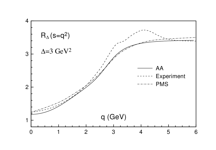
Figure 6: The quantity $R_{\Delta}(q^{2})$ corresponding to the parameter value $\Delta=3\,{\mbox{\rm GeV}}^{2}$. The figure shows the experimental curve, the result of the PMS-optimization of the third-order perturbative expansion obtained in [22], and the result of the analytic approach through the third order.

For $\Delta=3\,{\mbox{\rm GeV}}^{2}$, Fig. 6 shows the corresponding experimental curve and the curve found in [22] from the PMS-optimization of the third-order perturbative expansion. The same figure gives also the result of our calculation through the third order. For the scaling parameter in the analytic approach, we took the value $\Lambda_{\rm an}=870\,$MeV  ($f=3$) obtained from the analysis of the semileptonic $\tau$-decay in the APT framework. For the quark masses, we took the values that are close to the constituent ones (cf. [27]), $m_{u}=m_{d}=250\,$MeV,  $m_{s}=400\,$MeV,  $m_{c}=1.35\,$GeV,  $m_{b}=4.75\,$GeV and $m_{t}=174\,$GeV.

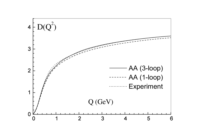
Figure 7: $D$-function.

New “experimental” data for the $D$-function were obtained recently [28]. We give in Fig. 7 the corresponding curves and also the result of our calculation. Figure 7 shows that good fit of the experimental data can be achieved already in the first order of APT. The same conclusion, as we have noted, is valid for $R_{\Delta}$ in the entire energy range [8]. We note here that loop stability is not observed in the standard approach using the PMS-optimization. Moreover, the whole “trick” is based here on higher approximations. Thus, the situation regarding the absence or the presence of the infrared fixed point that can emerge in scheme optimization of the perturbative expansion depends in an essential way on the quantity under consideration (i.e., is defined by the coefficients of the perturbative expansion) [29].

3.3 The dependence on the renormalization scheme

Inevitable termination of the PT series, i.e., the approximation of a physical quantity by one of its partial sums, leads to the known problem of the dependence of the results on the renormalization prescription. Thus, the partial sum of the PT series used in approximating a physical quantity bears a dependence on the choice of the renormalization scheme, which is the source of theoretical ambiguity in describing experimental data. In QCD, such ambiguity is the greater the smaller are the energy parameters characteristic of the process. To solve the stability problem of the results obtained, it is by far not enough to investigate only loop stability within a certain renormalization scheme; one should also consider the scheme stability of the results.

We discuss the scheme arbitrariness arising in the APT in the example of the $R$-ratio for the $e^{+}e^{-}$-annihilation process into hadrons. We consider a class of MS-like schemes and compare our results with those obtained in the perturbative analysis (see, for example, [30]).

In passing from one renormalization scheme to another, the coupling constant transforms as

$$a^{\prime}=a(1+v_{1}a+v_{2}a^{2}+\cdots).$$ (3.15)

We limit ourselves here to the three-loop level of the $D$-function achieved at present, with the QCD corrections taken in the approximation where

$$d=a(1+d_{1}a+d_{2}{a}^{2}),$$ (3.16)

with the running charge determined as a solution of the renormalization group equation with the three-loop $\beta$-function

$$\beta(a)=\mu^{2}\frac{\partial a}{\partial\mu^{2}}=-ba^{2}(1+b_{1}a+b_{2}a^{2})\,,$$ (3.17)

where

$$b = \frac{33-2f}{6}\,,\qquad b_{1}=\frac{153-19f}{66-4f},$$ (3.18)

$$b_{2}^{\overline{\rm MS}} = \frac{77139-15099f+325f^{2}}{288(33-2f)}\,.$$

The three-loop $\beta$-function coefficient $b_{2}$ and the expansion coefficients $d_{1}$ and $d_{2}$ in (3.16) depend on the choice of the renormalization scheme. Under scheme transformation (3.15), they change as

$$b_{2}^{\prime} = b_{2}-v_{1}^{2}-b_{1}v_{1}+v_{2}\,,$$

$$d_{1}^{\prime} = d_{1}-v_{1}\,,$$ (3.19)

$$d_{2}^{\prime} = d_{2}-2(d_{1}-v_{1})v_{1}-v_{2}\,.$$

Thus, every term in representation (3.16) undergoes a transformation, and we thus obtain the new function

$$d^{\prime}=a^{\prime}(1+d_{1}^{\prime}a^{\prime}+d_{2}^{\prime}{a^{\prime}}^{2}),$$ (3.20)

where the coupling $a^{\prime}$ is evaluated with the new $\beta$-function, with the three-loop coefficient $b_{2}$ replaced by the primed one $b_{2}^{\prime}$.

Recalling the transformation law of the scaling parameter [31]

$$\Lambda^{\prime}=\Lambda\exp({v_{1}}/{b})$$

and Eqs. (3.3), we find two scheme invariants [25]

$$\rho_{1}=\frac{b}{2}\log\frac{Q^{2}}{\Lambda^{2}}-d_{1},\qquad\rho_{2}=b_{2}+d_{2}-b_{1}d_{1}-d_{1}^{2}.$$ (3.21)

We normalize the momentum scale at $\Lambda_{\overline{\rm MS}}$. In arbitrary scheme, the invariant charge is then determined from the equation

$$\frac{b}{2}\,\log\left(\frac{Q^{2}}{\Lambda_{\overline{\rm MS}}^{2}}\right)=d_{1}^{\overline{\rm MS}}-d_{1}+\Phi(a,b_{2})\,,$$ (3.22)

where

$$\Phi(a,b_{2})=\frac{1}{a}-b_{1}\log\frac{1+b_{1}a}{\beta_{0}a}+b_{2}\int_{0}^{a}\frac{dx}{(1+b_{1}x)(1+b_{1}x+b_{2}x^{2})}.$$ (3.23)

Although there are no general arguments to prefer a certain renormalization scheme from the start, we nevertheless can define a class of “natural” schemes, which look reasonable at the three-loop level that we consider. The relevant criterion was proposed in [32]. One should restrict oneself to the schemes where the cancellations between different terms in the second scheme invariant (3.21) are not too large. Quantitatively, this criterion can be related to the cancellation index

$$C=\frac{1}{|\rho_{2}|}\,\bigl{(}|b_{2}|+|d_{2}|+d_{1}^{2}+|d_{1}|b_{1}\bigr{)}\,.$$ (3.24)

One should of course keep in mind the conventions involved in these considerations, in particular as regards the minimal value of the cancellation index.

Given a certain maximum value of the cancellation index $C_{\max}$, we can investigate stability of the results obtained by taking different schemes with the index $C\leq C_{\max}$. As $C_{\max}$, we take the index corresponding to the optimal PMS-scheme. We then have a relatively small class of “admissible” schemes bounded by the maximal index $C_{\rm PMS}$.

For $R(s)$, the cancellation index $C_{R}$ is evaluated using the known coefficients $r_{1}$ and $r_{2}$ of the perturbative expansion of the correction $r=a(1+r_{1}a+r_{2}a^{2})$. For the PMS-scheme, it is $C_{\rm PMS}\simeq 2$. To demonstrate the scheme arbitrariness arising here, we choose two schemes from this class. The first one is the $H$ scheme with the parameters $r_{1}^{({\rm H})}=-3.2$ and $b_{2}^{({\rm H})}=0$ (the ’t Hooft scheme), and the second is the $\overline{\rm MS}$-scheme corresponding to the parameters $r_{1}^{(\overline{\rm MS})}=1.64$ and $b_{2}^{(\overline{\rm MS})}=4.47$. These schemes are close to each other and to the boundary cancellation index $C_{\rm H}\simeq C_{\overline{\rm MS}}\simeq C_{\rm PMS}\simeq 2$.

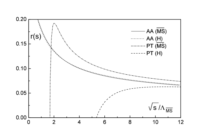
Figure 8: The graph of $r(s)$ calculated in perturbation theory (PT) and in the analytic approach (AA) for two renormalization schemes $H$ and $\overline{\rm MS}$ with the same cancellation index $C_{R}\simeq 2$.

Figure 8 shows the QCD correction $r(s)$ as a function of $\sqrt{s}/\Lambda_{\overline{\rm MS}}$ evaluated in perturbation theory and in the analytic approach for two renormalization schemes $H$ and $\overline{\rm MS}$ with approximately the same cancellation indices $C_{R}\simeq 2$. As can be seen from the figure, the analytic approach allows us to drastically reduce the scheme arbitrariness.

Essential reduction of the scheme dependence in the APT also takes place for other processes, for example the inclusive $\tau$-decay [11], and in the Bjorken and Gross–Llewellyn Smith sum rules for the inelastic lepton–hadron scattering [13, 14]. In the analytic approach, therefore, the three-loop level reached presently for a number of physical processes is practically invariant with respect to the choice of the renormalization prescription.

3.4 Inclusive $\tau$-lepton decay

The inclusive $\tau$-decay (see Fig. 9 for the corresponding diagram) allows one to perform a low-energy test of QCD. The $\tau$-lepton mass $M_{\tau}=1777^{+0.29}_{-0.26}\,$MeV [33], on the one hand, is sufficiently large to allow the hadronic decay modes, but on the other hand, is small in the chromodynamics scale, where it is in the low-energy domain. Theoretical description of the inclusive $\tau$-decay is in principle possible without any model assumptions, which is important for reliably determining the low-energy value of $\bar{\alpha}_{s}(M_{\tau}^{2})$ from experimental data. The main quantity to be studied is the $R_{\tau}$-ratio

$$R_{\tau}=\frac{\Gamma\bigl{[}\tau^{-}\to\nu_{\tau}+{\rm hadrons}(\gamma)\bigr{]}}{\Gamma\bigl{[}\tau^{-}\to\nu_{\tau}e^{-}\overline{\nu}_{e}(\gamma)\bigr{]}},$$ (3.25)

which in the modern experiments can be measures with the accuracy of several per cent.

Figure 9: The inclusive $\tau$-lepton decay diagram.

The starting point of the theoretical analysis is the expression

$$R_{\tau}=2\int_{0}^{M^{2}_{\tau}}\frac{ds}{M^{2}_{\tau}}\left(1-\frac{s}{M^{2}_{\tau}}\right)^{2}\left(1+\frac{2s}{M^{2}_{\tau}}\right)\widetilde{R}(s),$$ (3.26)

where $\widetilde{R}(s)$ is defined by the imaginary part of the hadron correlator

$$\Pi(s)=\sum_{q=d,s}{|V_{uq}|}^{2}\bigl{[}\Pi_{uq,V}(s)+\Pi_{uq,A}(s)\bigr{]}.$$ (3.27)

Here $V_{uq}$ are the Kobayashi–Maskawa matrix elements. In the massless case considered here, the vector and axial-vector hadron correlators, $\Pi_{uq,V}$ and $\Pi_{uq,A}$ respectively, coincide, and the function $\widetilde{R}(s)$ is equal to the ratio $R(s)$ for the $e^{+}e^{-}$-annihilation process into hadrons.

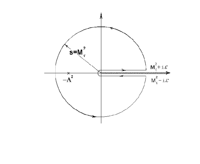
Figure 10: Transition to the contour representation for $R_{\tau}$.

The standard analysis of the $\tau$-decay immediately faces a difficulty in applying the original formula (3.26), because the parametrization of the function $R(s)$ by perturbative $\bar{\alpha}_{s}$ with the unphysical singularities leads to singularities in the integrand. The way out proposed in [34] consists in the following. Integral (3.26) is represented as a combination of integrals along the sides of the cuts in the $s$ complex plane (see Fig. 10). By the Cauchy theorem, this integral is then “transformed” into the integral along the contour $|s|=M_{\tau}^{2}$. After the integration by parts, we are left with the contour representation of $R_{\tau}$ involving the $D$-function,

$$R_{\tau}=\frac{1}{2\pi i}\oint_{|z|=1}\frac{dz}{z}{(1-z)}^{3}(1+z)D(M^{2}_{\tau}z).$$ (3.28)

The transition from the original expression (3.26) to contour representation (3.28) is based on certain analytic properties of the correlator, which are violated in the standard analysis. Thus, the proper analytic properties ensuring the analytic approach are important for the consistency of the inclusive $\tau$-decay description.

We describe this process in the APT [9]. We single out the strong-interaction contribution $\Delta_{\tau}$ to the $R_{\tau}$-ratio

$$R_{\tau}=R_{\tau}^{(0)}(1+\Delta_{\tau}),$$ (3.29)

where $R_{\tau}^{(0)}$ is a known factor including electroweak corrections.

We express $\Delta_{\tau}$ through the effective spectral function as

$$\Delta_{\tau}=\frac{d_{1}}{\pi}\int_{0}^{\infty}\frac{d\sigma}{\sigma}\rho^{\rm eff}(\sigma)-\frac{d_{1}}{\pi}\int_{0}^{M^{2}_{\tau}}\frac{d\sigma}{\sigma}{\left(1-\frac{\sigma}{M^{2}_{\tau}}\right)}^{3}{\left(1+\frac{\sigma}{M^{2}_{\tau}}\right)}\rho^{\rm eff}(\sigma).$$ (3.30)

Because of the universality property, the integral in the first term can be expressed through $a_{\rm an}(0)$. The spectral function in the two-loop approximation has the form

$$\rho^{\rm eff}(\sigma)=\varrho(\sigma)+\frac{1}{\beta_{0}^{2}}\frac{d_{2}}{d_{1}}\frac{2R(L)I(L)}{\bigl{[}R^{2}(L)+I^{2}(L)\bigr{]}^{2}},$$ (3.31)

where the spectral density of the invariant charge $\varrho(\sigma)$ is defined in (2.8) and the functions $R(L)$ and $I(L)$ are given by (2.9). Inserting (3.31) in (3.30) allows us to evaluate the strong-interaction contribution $\Delta_{\tau}$ in terms of the scale parameter $\Lambda$.

Using the experimental value $R_{\tau}=3.633\pm 0.031$ [33], we obtain $\alpha(M_{\tau}^{2})=0.400\pm 0.026$ and the corresponding value of the scaling parameter $\Lambda^{(3)}_{\rm an}=935\pm 159\,$MeV. These values are larger than those obtained in PT using the contour representation [35]. The reason lies in the fact that the nonperturbative corrections characteristic of the analytic approach give a negative contribution to $\Delta_{\tau}$ [9, 10]. Thus, to obtain the same value $\Delta_{\tau}$ in PT and in the analytic approach, the “perturbative component” contribution of the latter should be increased by increasing $\Lambda$. The inclusive $\tau$-decay was analyzed at the three-loop APT level in [36]. The corresponding value of $\Lambda$ turned out to be smaller, $\Lambda^{(3)}_{\rm an}=871\pm 155\,$MeV. The scheme stability of this analysis was also shown in [36]. It should be noted that the quantity $\Lambda_{\rm an}$ is very sensitive to the experimental value of $R_{\tau}$. Thus, using $R_{\tau}=3.559\pm 0.035$  [37], we obtain $\Lambda^{(3)}_{\rm an}=640\pm 127\,$MeV, which corresponds to a considerably smaller invariant charge at the mass $M_{\tau}$ (see Table 1).

4 The analytic approach in inelastic lepton-hadron scattering

In this section, we give a theoretical foundation of a possible application of our analytic description to inelastic lepton–hadron scattering processes. The key point of our construction—the analytic properties of the structure function moments with respect to  $Q^{2}$—requires a certain modification of the standard formalism, in particular, the change of the standard Bjorken moments $M_{n}(Q^{2})$ with the modified moments ${\cal M}_{n}(Q^{2})$ with respect to a new scaling variable that takes kinematic mass dependence into account. We start with the Jost–Lehmann integral representation (see, for example, § 55 of [5]) for the Fourier image of the corresponding matrix element.

4.1 The Jost–Lehmann representation

The structure functions of the inelastic lepton–hadron scattering depend on two arguments, and the corresponding representations that accumulate the fundamental properties of the theory (such as relativistic invariance, spectrality, and causality) have a more complicated form in our analysis than in representations for functions of one variable. Two such representations are known in the literature. We use the 4-dimensional integral representation proposed by Jost and Lehmann [38] for the so-called symmetric case. Applications of this representation to automodel asymptotic structure functions were considered by Bogoliubov, Vladimirov, and Tavkhelidze [4], some of whose results and notation we use in what follows. The proof of the Jost–Lehmann representation is based on the most general properties of the theory, such as covariance, Hermiticity, spectrality, and causality (see [5]; some mathematical problems related to the Jost–Lehmann–Dyson representation are also considered in [40, 41]).

For definiteness, we speak about the inelastic scattering of charged leptons (electrons, muons) on nucleons, i.e., we consider the process $\ell+N\rightarrow\ell+hadrons$. In the lowest order in the electromagnetic coupling constant (one-photon exchange), this process is shown in Fig. 11, which also explains our notation. In the unpolarized case, the cross-section of the process is defined by the hadronic tensor

$$W_{\mu\nu}(q,P)=\frac{1}{4\pi}\sum_{\sigma}\int dx\,\exp(iq\cdot x)\left\langle P,\sigma\left|\left[J_{\mu}\left(\frac{x}{2}\right),J_{\nu}\left(-\frac{x}{2}\right)\right]\right|P,\sigma\right\rangle$$ (4.1)

constructed of the commutators of the currents, with the sum taken over the nucleon polarizations.

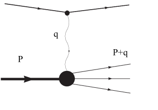
Figure 11: The deep inelastic lepton–hadron scattering diagram in the one-photon exchange approximation.

Relativistic invariance and the electromagnetic current conservation lead to the parametrization of tensor (4.1) in terms of two structure functions $w_{1}$ and $w_{2}$,

$$W_{\mu\nu}(q,P) = \left(-g_{\mu\nu}+\frac{q_{\mu}q_{\nu}}{q^{2}}\right)w_{1}(q,P)$$

$$+ \frac{1}{M^{2}}\left(p_{\mu}-\frac{P\cdot q}{q^{2}}q_{\mu}\right)\left(p_{\nu}-\frac{P\cdot q}{q^{2}}q_{\nu}\right)w_{2}(q,P)\,,$$

where $M=\sqrt{P^{2}}$ is the nucleon mass.

We now list the main properties of the functions $w$ following from the general principles of local QFT:

– covariance property means that the functions $w$ depend on two scalar arguments, which we choose as $\nu=P\cdot q$ and $Q^{2}=-q^{2}$,

$$w(q,P)=W(\nu,Q^{2});$$

– spectrality property is written as

$$W(\nu,Q^{2})=0\qquad{\rm for}\qquad\frac{Q^{2}}{2\nu}=x>1,$$

where we used the dimensionless Bjorken variable, which in the physical domain of the process for $(q+P)^{2}>M^{2}$ is kinematically restricted by the interval $0<x<1$;

– the structure function parametrizes the scattering cross-section and is real (the reality property),

$$W(\nu,Q^{2})=W^{*}(\nu,Q^{2});$$

– Hermiticity of the current operator leads to the (anti-)symmetry property

$$W(-\nu,Q^{2})=-W(\nu,Q^{2});$$

– the vanishing of the commutator of currents at space-like intervals because of the local commutativity of currents gives the causality condition

$$\int\frac{dq}{(2\pi)^{4}}\exp(-iqz)W(q,P)=0\qquad{\rm for}\qquad z^{2}<0.$$

For the function $W(\nu,Q^{2})$ satisfying all these conditions, there exists a real moderately growing distribution $\psi({\bf u},\lambda^{2})$ such that the Jost–Lehmann integral representation holds; in the nucleon rest frame, this can be written as [4]

$$W(\nu,Q^{2})=\varepsilon(q_{0})\int d{\bf u}\,d\lambda^{2}\,\delta\bigl{[}q_{0}^{2}-(M{\bf u}-{\bf q})^{2}-\lambda^{2}\bigr{]}\psi({\bf u},\lambda^{2}),$$ (4.3)

with the function $\psi({\bf u},\lambda^{2})$ supported on the set

$$\rho=|{\bf u}|\leq 1,\qquad\lambda^{2}\geq M^{2}\bigl{(}1-\sqrt{1-\rho^{2}}\,\bigr{)}^{2}.$$

For the process under consideration, the physical values of $\nu$ and $Q^{2}$ are positive. We, thus, can neglect the factor $\varepsilon(q_{0})=\varepsilon(\nu)$ and keep the same notation for $W(\nu,Q^{2})$. Taking into account that the weight function $\psi({\bf u},\lambda^{2})=\psi(\rho,\lambda^{2})$ is radial-symmetric, as follows from covariance [4], we write the Jost–Lehmann representation for $W$ in the covariant form,

$$W(\nu,Q^{2}) = \int_{0}^{1}d\rho\,\rho^{2}\int_{\lambda_{\min}^{2}}^{\infty}d\lambda^{2}\int_{-1}^{1}dz$$

$$\times \delta\bigl{(}Q^{2}+M^{2}\rho^{2}+\lambda^{2}-2z\rho\sqrt{\nu^{2}+M^{2}Q^{2}}\,\bigr{)}\psi(\rho,\lambda^{2})\,,$$

where

$$\lambda_{\min}^{2}=M^{2}\bigl{(}1-\sqrt{1-\rho^{2}}\,\bigr{)}^{2}.$$ (4.5)

4.2 Analytic moments of the structure functions

As follows from representation (4.1), a natural scaling variable is given by

$$s=\frac{1}{2}\sqrt{\frac{Q^{2}(Q^{2}+4M^{2})}{\nu^{2}+M^{2}Q^{2}}}\,=x\sqrt{\frac{Q^{2}+4M^{2}}{Q^{2}+4M^{2}x^{2}}}\,,$$ (4.6)

which accumulates the root structure determined by the $\delta$-function argument. At the same time, in the physical region of the process, the $s$ variable changes in the same way as the Bjorken variable $x$, i.e., from zero to one. The variable $s$ bears a dependence on the mass of the target (the nucleon) and is different from both the Bjorken variable and the Nachtmann variable [42]

$$\xi=\frac{2x}{1+\sqrt{1+x^{2}4M^{2}/Q^{2}}}$$

that is sometimes used in the kinematical account of mass effects of inelastic scattering processes. However, only the $s$ variable leads to the moments that have the analytic properties in $Q^{2}$ that we need.

To establish these properties, we integrate over $z$ in (4.1) as

$$W(\nu,Q^{2}) = \frac{s}{Q^{2}\sqrt{1+4M^{2}/Q^{2}}}\int_{0}^{1}d\rho\,\rho\int_{\lambda_{\min}^{2}}^{\infty}d\lambda^{2}$$

$$\times \theta\left[Q^{2}\rho^{2}-s\frac{(Q^{2}+M^{2}\rho^{2}+\lambda^{2})}{\sqrt{1+4M^{2}/Q^{2}}}\right]\,\psi(\rho,\lambda^{2}).$$

We now define the modified $s$-moments of the structure functions (cf. [43])

$${\cal M}_{n}(Q^{2})=\frac{1}{{(1+4M^{2}/Q^{2})}^{(n-1)/2}}\int\limits_{0}^{1}dss^{n-2}W(\nu,Q^{2})\,.$$ (4.8)

Inserting $W(\nu,Q^{2})$ as given by (4.2), we obtain

$${\cal M}_{n}(Q^{2})=\frac{(Q^{2})^{n-1}}{n}\int_{0}^{1}d\rho\,\rho^{n+1}\int_{0}^{\infty}d\sigma\frac{\theta(\sigma-\sigma_{\min})}{(Q^{2}+\sigma)^{n}}\psi(\rho,\sigma-M^{2}\rho^{2}),$$

where $\sigma=\lambda^{2}+M^{2}\rho^{2}$ and $\sigma_{\min}=2M^{2}\bigl{(}1-\sqrt{1-\rho^{2}}\,\bigr{)}$.

Introducing the weight function

$$m_{n}(\sigma)=\frac{1}{n}\int_{0}^{1}d\rho\,\rho^{n+1}\theta(\sigma-\sigma_{\min})\,\psi(\rho,\sigma-M^{2}\rho^{2}),$$ (4.9)

we obtain the representation for the $s$-moments

$${\cal M}_{n}(Q^{2})=(Q^{2})^{n-1}\int_{0}^{\infty}d\sigma\frac{m_{n}(\sigma)}{(\sigma+Q^{2})^{n}},$$ (4.10)

which implies the analyticity of ${\cal M}_{n}(Q^{2})$ in the complex $Q^{2}$ plane cut along the negative semi-axis, i.e., the Källén–Lehmann type analyticity.

In [44], the Deser–Gilbert–Sudarshan integral representation [45] was used to arrive at a similar statement regarding the analyticity of the Källén–Lehmann type for the $x$-moments. However the status of this representation in QFT is less clear, since it cannot be obtained starting with only the basic principles of the theory.

The relation between moments (4.8) and the standard Bjorken moments

$$M_{n}(Q^{2})=\int_{0}^{1}dx\,x^{n-2}W(\nu,Q^{2})$$ (4.11)

can be expressed by

$${\cal M}_{n}(Q^{2}) = \frac{1}{\Gamma[(n+1)/2]}\,\sum\limits_{k=0}^{\infty}\frac{\Gamma[k+(n+1)/2]}{k!}\left(-\frac{4M^{2}}{Q^{2}}\right)^{k}M_{n+2k}(Q^{2})\,,$$

$$M_{n}(Q^{2}) = \frac{1}{\Gamma[(n+1)/2]}\,\sum\limits_{k=0}^{\infty}\frac{\Gamma[k+(n+1)/2]}{k!}\left(\frac{4M^{2}}{Q^{2}}\right)^{k}{\cal M}_{n+2k}(Q^{2})\,.$$

In the asymptotic domain corresponding to large values of the transferred momentum $Q^{2}$, where power corrections of the form $1/(Q^{2})^{n}$ can be neglected, the $x$-, $s$-, and $\xi$-moments are identical. Outside the asymptotic domain, on the other hand, where it comes to studying the contribution of higher twists, the difference between these definitions of moments must be taken into account.

4.3 Dispersion relation and the operator product expansion

To establish the relation with the operator product expansion, we start with the Jost–Lehmann representation and obtain a dispersion relation for the forward Compton scattering amplitude with respect to the new variable (4.6). We write the matrix element of the process corresponding to representation (4.1) as

$$T(\nu,Q^{2}) = \frac{1}{\pi}\int_{0}^{1}d\rho\,\rho^{2}\int_{\lambda_{\min}^{2}}^{\infty}d\lambda^{2}\int_{-1}^{1}\,dz$$

$$\times \frac{\psi(\rho,\lambda^{2})}{Q^{2}+M^{2}\rho^{2}+\lambda^{2}-2z\rho\sqrt{\nu^{2}+M^{2}Q^{2}}\,-i\epsilon}.$$

In the complex $\nu^{2}$ plane, the function $T(\nu,Q^{2})$ has a branch cut along the positive part of the real axis starting at $\nu^{2}_{\min}$ defined by the condition

$$\sqrt{\nu^{2}_{\min}+M^{2}Q^{2}}\,=\min_{\{\lambda,\rho,z\}}\left|\frac{Q^{2}+M^{2}\rho^{2}+\lambda^{2}}{2z\rho}\right|.$$

Recalling (4.5) and the range of the integration variable $z$ in (4.3), we can simplify this to

$$\sqrt{\nu^{2}_{\min}+M^{2}Q^{2}}\,=\min_{\{\rho\}}\frac{Q^{2}+2M^{2}\bigl{(}1-\sqrt{1-\rho^{2}}\,\bigr{)}}{2\rho},$$ (4.13)

which leads to $\nu^{2}_{\min}=(Q^{2}/2)^{2}$. Thus, the sought dispersion relation has the form

$$T(\nu,Q^{2})=\frac{1}{\pi}\int_{Q^{4}/4}^{\infty}\frac{d\nu_{1}^{2}}{\nu_{1}^{2}-\nu^{2}-i\epsilon}W(\nu_{1},Q^{2}).$$ (4.14)

We note that in terms of the Bjorken variable $x$, relation (4.14) is represented as

$$T(\nu,Q^{2})=\frac{2}{\pi}\int_{0}^{1}\frac{dx_{1}}{x_{1}}\frac{1}{1-(x_{1}/x)^{2}}\,W(\nu_{1},Q^{2}).$$ (4.15)

This expression determines simple properties of the amplitude $T(x,Q^{2})$ in the complex $x$-plane and is convenient in the operator product expansion.

In considering consequences of the Jost–Lehmann representation, as noted above, the natural scaling variable is given by $s$. In this case, there arises a similar structure of the dispersion integral 

$$T(\nu,Q^{2})=\frac{2}{\pi}\int_{0}^{1}\frac{ds_{1}}{s_{1}}\frac{1}{1-(s_{1}/s)^{2}}\,W(\nu_{1},Q^{2});\qquad\nu^{2}=Q^{2}\left[\frac{Q^{2}+4M^{2}}{4s^{2}}-M^{2}\right].$$ (4.16)

The identity between the structures of the dispersion relations with respect to the variables $x$ and $s$ allows us to establish the relation of analytic moments (4.8) to the operator product expansions of currents used in finding the $Q^{2}$-evolution of the structure functions of the moments. The moments in Eq. (4.11) correspond to the case where only the Lorentz structures of the form $P_{\mu_{1}}\dots P_{\mu_{n}}$ are taken into account in matrix elements of the operator $\bigl{\langle}P|\widehat{O}_{\mu_{1}\dots\mu_{n}}|P\bigr{\rangle}$. Then the application of the operator product expansion for the Compton amplitude leads to the expansion in powers of $(q\cdot P)/Q^{2}$, i.e., to the expansion in the inverse powers of $x$. A similar expansion in the inverse powers of $x$ can also be done in dispersion integral (4.15). The coefficients are then determined by the $x$-moments. Comparing the two power series gives the sought relation between the $x$-moments and the operator product expansion.

In the general case, the symmetric matrix element $\bigl{\langle}P|\widehat{O}_{\mu_{1}\dots\mu_{n}}|P\bigr{\rangle}$ contains the Lorentz structures given by $\{P_{\mu_{1}}\dots P_{\mu_{n}}\}$,  $M^{2}g_{\mu_{i}\mu_{j}}\{P_{\mu_{1}}\dots P_{\mu_{n-2}}\}$, etc. The moments with respect to the $\xi$ variable correspond to choosing the operator basis where the expansion goes over traceless tensors, i.e., such that the contraction of $g_{\mu_{i}\mu_{j}}$ with $\bigl{\langle}P|\widehat{O}_{\mu_{1}\dots\mu_{n}}|P\bigr{\rangle}$ vanishes for any two indices. It is then obvious that the Lorentz structure of the matrix element $\bigl{\langle}P|\widehat{O}_{\mu_{1}\dots\mu_{n}}|P\bigr{\rangle}$ is fixed unambiguously.

Dispersion representation (4.16) allows us to expand the Compton amplitude in the inverse powers of $s$. If the operator basis is chosen such that an arbitrary contraction of the tensor $\bigl{\langle}P|\widehat{O}_{\mu_{1}\dots\mu_{n}}|P\bigr{\rangle}$ with the nucleon momentum $P_{\mu_{i}}$ vanishes, then the operator product expansion leads to a power series for the forward Compton scattering amplitude with the expansion parameter $q_{\mu}q_{\nu}(P_{\mu}P_{\nu}-g_{\mu\mu}P^{2})/(q^{2})^{2}$, which corresponds to expanding dispersion integral (4.16) in powers of $1/s^{2}$. We thus arrive at the relation between the analytic $s$-moments and the operator product expansion. We stress that the orthogonality requirement of the symmetric tensor $\bigl{\langle}P|\widehat{O}_{\mu_{1}\dots\mu_{n}}|P\bigr{\rangle}$ to the nucleon momentum $P_{\mu_{i}}$ determines its Lorentz structure unambiguously.

5 Conclusions

We considered the analytic formulation of QCD, where the analyticized RG-solutions for the invariant coupling functions, the Green’s functions, and the matrix elements are free of unphysical singularities. An important property of this formulation that we found is the stability of the analytic invariant charge with respect to higher-loop correction in all of the $Q^{2}$ range. The key point here is the existence of the universal limiting value $\bar{\alpha}_{\rm an}(0)=4\pi/\beta_{0}$ that is invariant with respect to multiloop corrections. This constant is independent of the $\Lambda_{\rm{QCD}}$ parameter and is determined only by the general symmetry properties of the Lagrangian. Therefore, the family of curves $\bar{\alpha}_{\rm an}(Q^{2}/\Lambda^{2})$ for different values of the $\Lambda$ parameter is a bundle with the common point $\bar{\alpha}_{\rm an}(0)=4\pi/\beta_{0}$ (this picture is independent of the number of loops).

The invariant analytic formulation essentially modifies the behavior of $\bar{\alpha}_{\rm an}(x)$ in the IR region by making it stable with respect to higher-loop corrections. The two-loop approximation differs from the one-loop one by no more than $\simeq 10\,\%$ in the small-$Q^{2}$ domain, and the three-loop approximation differs from the two-loop one by only $\simeq 1\,\%$. This is radically different from the situation encountered in the standard renormalization-group PT, which is characterized by strong instability with respect to the next loop corrections in the domain of small $Q^{2}\simeq\Lambda^{2}$. We note also that maintaining the proper analytic properties with respect to $Q^{2}$ is essential for a self-consistent definition of the effective coupling function in the time-like region [15]. In describing the concrete processes, for example the inclusive $\tau$-lepton decay, a consistent analysis is possible [9] only provided the above analytic properties hold.

There are at least two possibilities to describe physical quantities in the new approach framework. The simplest one consists in replacing $\bar{\alpha}_{s}(x)\to\bar{\alpha}_{\rm an}(x)$ in the explicit expressions for the observables “processed” by the RG method, or more precisely, for the related quantities defined in the space-like region of the $Q^{2}$ variable.

We take another possibility, however. For the quantities similar to the Adler $D(Q^{2})$-function that are represented by the PT power series, according to a special convention, the analyticization procedure is applied to each power of $\bar{\alpha}_{s}(Q^{2})$ separately. This leads to a new non-power-series expansion, in which the powers of $\bar{\alpha}_{s}(Q^{2})$ are replaced with new nonsingular functions of $A_{n}(Q^{2})$. We call this algorithm, which was first proposed in [9], the APT. Applying this algorithm to analyze the amplitudes of the processes like the $e^{+}e^{-}$-annihilation into hadrons and the inclusive $\tau$-decay, and also of the sum rules for the inelastic lepton–hadron scattering, we see that in addition to possessing loop stability, the APT results are much less sensitive to the choice of the renormalization scheme than in the standard approach. In other words, the three-loop APT level practically insures both the loop saturation and the scheme invariance of the relevant physical quantities in the entire energy or momentum range.

It appears that by accounting for the additional information about the proper analytic properties, the first terms of the APT non-power-series expansion already give sufficiently good approximation to the sum of the whole series. We recall here the analogy with summing up the perturbative expansions with the additional information on the behavior of the remote PT series terms taken into account [46]. In that case, it also turned out that the expression for the approximated function given by the first several terms of the loop expansion was practically unchanged by higher corrections.

In this work, we considered also the structure functions of the inelastic lepton–hadron scattering, which are more complicated objects than the two-point functions, which are in one way or another related with the Källén–Lehmann representation. For these functions, the general quantum field theory principles, including covariance, Hermiticity, spectrality, and causality, are expressed by the Jost–Lehmann–Dyson integral representation. In using the analytic approach to define the $Q^{2}$-evolution, it was convenient to introduce the moments ${\cal M}_{n}(Q^{2})$ of the structure functions corresponding to the special scaling variable (4.6). It is these moments, rather than the Bjorken or Nachtmann ones, that exhibits simple analytic properties with respect to $Q^{2}$. In this work, we found the relation of the new analytic moments ${\cal M}_{n}(Q^{2})$ to the operator product expansion, where the tensor structure of the matrix elements of operators with respect to the nucleon states must be fixed according to the condition that they be orthogonal to the nucleon momentum.

Acknowledgments

It is a pleasure to thank V. S. Vladimirov, A. V. Efremov, B. I. Zav’yalov, V. A. Meshcheryakov, S. V. Mikhailov, K. A. Milton, O. V. Teryaev, and O. P. Solovtsova for useful discussions of the results. We are also grateful to the Russian Foundation for Basic Research (Grants No. 96-15-96030 and No. 99-01-00091) and INTAS (Grant No. 96-0842) for support.

References

- [1] N.N. Bogoliubov and D.V. Shirkov, Dokl. Akad. Nauk SSSR 103, 203 (1955); 391.
- [2] N. N. Bogoliubov and D. V. Shirkov, JETP 30, 77 (1956); Nuovo Cim. 3, 845 (1956).
- [3] N. N. Bogolyubov, A. A. Logunov, and D. V. Shirkov, JETP 37, 805 (1959).
- [4] N. N. Bogolyubov, V. S. Vladimirov, and A. N. Tavkhelidze, Theor. Math. Phys. 12, 3 (1972); 305.
- [5] N. N. Bogoliubov and D. V. Shirkov, Introduction to the Theory of Quantum Fields (Chap. “Desipersion Relations”) [in Russian], Nauka, Moscow (1973, 1976, 1986); English transl.: Wiley, New York (1959, 1980).
- [6] D. V. Shirkov and I. L. Solovtsov, JINR Rap. Comm. 2 [76], 5 (1996); “Analytic QCD running coupling with finite IR behavior and universal value”, hep-ph/9604363.
- [7] D. V. Shirkov and I. L. Solovtsov, Phys. Rev. Lett. 79, 1209 (1997).
- [8] I. L. Solovtsov and D. V. Shirkov, Phys. Lett. B 442, 344 (1998).
- [9] K. A. Milton, I. L. Solovtsov, and O. P. Solovtsova, Phys. Lett. B 415, 104 (1997).
- [10] O. P. Solovtsova, JETP Lett. 64, 664 (1996).
- [11] K. A. Milton, I. L. Solovtsov, and O. P. Solovtsova, “Analytic Perturbative Approach to QCD”, Talk given at the XXIX Int. Conference on HEP, Vancouver, B. C., Canada, July 23-29, 1998 (to be published in the Proceed.); Preprint OKHEP-98-06, Oklahoma, Oklahoma Univ. (1998); hep-ph/9808457.
-
[12]
D. V. Shirkov,
Nucl. Phys. B (Proc. Suppl.) 64, 106 (1998), hep-ph/9708480;
Theor. Math. Phys. 19, 438 (1999); “Renormalization group, causality, and nonpower perturbation expansion in QFT”; Preprint E2-98-311, JINR, Dubna (1998); hep-th/9810246. - [13] K. A. Milton, I. L. Solovtsov, and O. P. Solovtsova, Phys. Lett. B 439, 421 (1998).
- [14] K. A. Milton, I. L. Solovtsov, and O. P. Solovtsova, Phys. Rev. D 60 016001 (1999); Preprint OKHEP-98-07, Oklahoma, Oklahoma Univ. (1998); hep-ph/9809513.
- [15] K. A. Milton and I. L. Solovtsov, Phys. Rev. D 55, 5295 (1997).
- [16] K. A. Milton and O. P. Solovtsova, Phys. Rev. D 57, 5402 (1998).
- [17] I. F. Ginzburg and D. V. Shirkov, JETP 22, 234 (1966).
- [18] D. V. Shirkov, Nucl. Phys. B 332, 425 (1990).
- [19] D. V. Shirkov, Lett. Math. Phys. 1, 179 (1976).
- [20] B. A. Magradze, “The gluon propagator in analytic perturbation theory”, Talk given at 10th Intern. Seminar on High-Energy Physics (Quarks 98), Suzdal, Russia, 18-24 May, 1998; Preprint G-TMI-98-08-01, Tbilisi, TMI (1998); hep-ph/9808247.
- [21] E. Gardi, G. Grunberg, and M. Karliner, “Can the QCD running coupling have a causal analyticity structure?”, Preprint TAUP-2503-98, Paris, TAUP (1998); hep-ph/9806462.
- [22] A. C. Mattingly and P. M. Stevenson, Phys. Rev. D 49, 437 (1994).
- [23] Yu. L. Dokshitzer, V. A. Khoze, and S. I. Troyan, Phys. Rev. D 53, 89 (1996).
- [24] E. C. Poggio, H. R. Quinn, and S. Weinberg, Phys. Rev. D 13, 1958 (1976).
- [25] P. M. Stevenson, Phys. Rev. D 23, 2916 (1981).
- [26] S. G. Gorishny, A. L. Kataev, and S. A. Larin, Phys. Lett. B 259, 144 (1991).
- [27] F. Jegerlehner, Nucl. Phys. C (Proc. Suppl.) 51, 131 (1996); “Hadronic vacuum polarization contribution to of the leptons and ”, DESY Preprint 96-121, Hamburg, DESY (1996); hep-ph/9606484.
- [28] S. Eidelman, F. Jegerlehner, A. L. Kataev, and O. Veretin, Phy. Lett. B 454, 369 (1999); “Testing nonperturbative strong interaction effects via the Adler function”, Preprint DESY 98-206, Hamburg, DESY (1998); hep-ph/9812521.
- [29] J. Chyla, A. L. Kataev, and S. A. Larin, Phys. Lett. B 261, 269 (1991).
- [30] P. A. Ra̧czka and A. Szymacha, Phys. Rev. D 54, 3073 (1996).
- [31] W. Celmaster and R. J. Gonsalves, Phys. Rev. D 20, 1420 (1979).
- [32] P. A. Ra̧czka, Z. Phys. C 65, 481 (1995).
- [33] Particle Data Group, Phys. Rev. D 54, 1 (1996); Eur. Phys. J. C 3, 1 (1998).
- [34] E. Braaten, Phys. Rev. Lett. 60, 1606 (1988); Phys. Rev. D 39, 1458 (1989).
- [35] E. Braaten, S. Narison, and A. Pich, Nucl. Phys. B 373, 581 (1992).
- [36] K. A. Milton, I. L. Solovtsov, and V. I. Yasnov, “Analytic perturbation theory and renormalization scheme dependence in -decay”, Preprint OKHEP-98-01, Oklahoma, Oklahoma Univ. (1998); hep-ph/9802262.
- [37] T. Coan et al. (CLEO Collaboration), Phys. Lett. B 356, 580 (1996).
- [38] R. Jost and H. Lehmann, Nuovo Cim. 5, 1598 (1957).
- [39] F. J. Dyson, Phys. Rev. 110, 1460 (1958).
- [40] N. N. Bogoliubov, A. A. Logunov, A. I. Oksak, and I. T. Todorov, General Principles of Quantum Field Theory [in Russian], Nauka, Moscow (1987); English transl.: Dordrecht, Kluwer (1990).
- [41] V. S. Vladimirov, Yu. N. Drozhzhinov, and B. I. Zav’yalov, Tauberian Theorems for General Functions [in Russian], Nauka, Moscow (1986); English transl.: Dordrecht, Kluwer (1988).
- [42] O. Nachtmann, Nucl. Phys. B 63, 237 (1973).
- [43] B. Geyer, D. Robaschik, and E. Wieczorek, Fortschr. Phys. 27, 75 (1979); Fiz. Èlementar. Chastits i Atom. Yadra 11, 132 (1980).
- [44] W. Wetzel, Nucl. Phys. B 139, 170 (1978).
- [45] S. Deser, W. Gilbert, and E. C. S. Sudarshan, Phys. Rev. 117, 266 (1960).
- [46] D. I. Kazakov, O. V. Tarasov, and D. V. Shirkov, Theor. Math. Phys. 38, 9 (1979); D. I. Kazakov and D. V. Shirkov, Fortschr. Phys. 28, 465 (1980).