Trojan Penguins and Isospin Violation in Hadronic B Decays

Abstract:

Some rare hadronic decays of $B$ mesons, such as $B\to\pi K$, are sensitive to isospin-violating contributions from physics beyond the Standard Model. Although commonly referred to as electroweak penguins, such contributions can often arise through tree-level exchanges of heavy particles, or through strong-interaction loop diagrams. The Wilson coefficients of the corresponding electroweak penguin operators are calculated in a large class of New Physics models, and in many cases are found not to be suppressed with respect to the QCD penguin coefficients. Several tests for these effects using observables in $B^{\pm}\to\pi K$ decays are discussed, and nontrivial bounds on the couplings of the various New Physics models are derived.

1 Introduction

The study of rare decay processes is an important tool in testing the fundamental interactions among elementary particles, exploring the origin of CP violation, and searching for New Physics beyond the Standard Model (SM). Such processes have been explored in great detail, both theoretically and in experimental searches, in the weak interactions of kaons and $B$ mesons, as well as in $K$–$\bar{K}$, $D$–$\bar{D}$, and $B$–$\bar{B}$ mixing. Two prominent examples are the evidence for mixing-induced CP violating in the decay $B\to J/\psi\,K_{S}$ reported by the CDF Collaboration [1], and the observation of direct CP violation in the decays $K\to\pi\pi$ [2, 3], which has recently been confirmed by the KTeV and NA48 Collaborations [4, 5].

Flavor-changing neutral current (FCNC) processes, which are forbidden at tree level in the SM, are especially sensitive to any new source of flavor-violating interactions. Already, the absence of experimental signals for new FCNC couplings puts stringent bounds on the parameters of many extensions of the SM such as Supersymmetry (SUSY) [6]. So far, FCNC processes have been explored mainly in particle–antiparticle mixing and in “semihadronic” weak decays, which permit a clean theoretical description. In the kaon system, examples of the latter type are the decays $K\to\pi\,l^{+}l^{-}$ and $K\to\pi\,\nu\bar{\nu}$. In the $B$ system, the decays that have received the most attention are $B\to X_{s}\,\gamma$, $B\to X_{s}\,l^{+}l^{-}$ and $B\to X_{s}\,\nu\bar{\nu}$, where $X_{s}$ can be any final state, exclusive or inclusive, containing a strange quark [7].

In the present paper, we explore in detail how New Physics could affect purely hadronic decays such as $B\to\pi K$, which are sensitive to isospin- or, more generally, SU(3) flavor-violating interactions. In the SM, the main contributions to the decay amplitudes for these processes come from the penguin-induced FCNC transition $\bar{b}\to\bar{s}q\bar{q}$, which by far exceeds a small, Cabibbo-suppressed $\bar{b}\to\bar{u}u\bar{s}$ contribution from $W$-boson exchange. Because of a fortunate interplay of isospin, Fierz and flavor symmetries, the theoretical description of the charged decays $B^{\pm}\to\pi K$ in the SM is clean despite the fact that these are exclusive nonleptonic decays [8, 9]. Isospin violation arises through the small charged-current contribution and through the electroweak penguin operators in the low-energy effective weak Hamiltonian [10]. In the SM, these operators are induced by penguin and box diagrams involving the exchange of weakly interacting $W$ and $Z$ bosons, or of a photon. Here we point out that in a large class of New Physics models such effects can be mediated by “trojan” electroweak penguins, which are neither (pure) penguins nor of electroweak origin. Nevertheless, at low energies their effects are parameterized by an extension of the usual basis of electroweak penguin operators. We will explore examples where trojan penguins are induced by tree-level couplings, e.g., models with an extra $Z^{\prime}$ boson, or pure strong-interaction processes, e.g., gluino box diagrams in SUSY models.

In the present work we calculate the Wilson coefficients of the hadronic electroweak penguin operators in the effective weak Hamiltonian in an extended operator basis and for a large class of New Physics models. We then explore the phenomenological consequences of these new, isospin-violating contributions for weak-interaction observables. This serves two purposes: first, it allows us to derive bounds on New Physics parameters, which in some cases improve upon existing bounds derived from other processes; secondly, it shows which observables may be interesting to look at as far as searches for New Physics are concerned. We shall address both issues in detail for the particular case of $B^{\pm}\to\pi K$ decays, which in the context of the SM are of prime importance in determining the weak phase $\gamma=\mbox{arg}(V_{ub}^{*})$ of the Cabibbo–Kobayashi–Maskawa (CKM) matrix [8, 9, 11, 12, 13, 14]. We stress, however, that trojan penguins could be important in a much wider class of processes. In particular, they may be responsible for a large contribution to the quantity $\epsilon^{\prime}/\epsilon$ measuring direct CP violation in $K\to\pi\pi$ decays [15, 16]. The importance of $B^{\pm}\to\pi K$ decays in the search for New Physics has been emphasized in [9, 17], and some specific scenarios containing new isospin-violating contributions have been explored in [18, 19].

In Section 2, we discuss the effective weak Hamiltonian relevant to hadronic $B$ decays. In the presence of generic New Physics contributions, the basis of penguin operators has to be extended from the standard one in several aspects. We discuss the structure of the new operators and their scaling properties under a renormalization-group transformation from a high scale down to low energies. The theory of the rare hadronic decays $B^{\pm}\to\pi K$ is discussed in Section 3, where we indicate how various observables in these decays can be used to test for physics beyond the SM. We derive model-independent bounds on a ratio $R_{*}$ of CP-averaged $B^{\pm}\to\pi K$ branching ratios in the presence of New Physics, and show that the value $\gamma_{\pi K}$ of the weak phase extracted in $B\to\pi K$ decays is extremely sensitive to isospin-violating New Physics contributions. Because the theoretical analysis has only small hadronic uncertainties, potential New Physics effects can be detected even if they are 50% smaller than the isospin-violating contributions present in the SM. In Sections 4 and 5, we calculate the Wilson coefficients of the $\bar{b}\to\bar{s}q\bar{q}$ penguin operators in a large class of extensions of the SM, including models with tree-level FCNC couplings of the $Z$ boson, extended gauge models, multi-Higgs models, and SUSY models with and without R-parity conservation. In each case, we explore which region of parameter space can be probed by measuring certain $B^{\pm}\to\pi K$ observables, and how big a departure from the SM predictions one can expect under realistic circumstances. Section 6 contains a summary of our results and the conclusions.

2 Effective Hamiltonian for hadronic FCNC processes

The effective weak Hamiltonians relevant to rare hadronic $B$ decays based on the quark transitions $\bar{b}\to\bar{s}q\bar{q}$ or $\bar{b}\to\bar{d}q\bar{q}$ have been discussed extensively in the literature. Here we consider only the first case, adopting the notations of [10]. A similar discussion (with obvious replacements of indices) would apply to the other case. In the SM, the result can be written in the compact form

$${\cal H}_{\rm eff}=\frac{G_{F}}{\sqrt{2}}\,\sum_{q=u,c}\lambda_{q}\,\bigg{[}\sum_{i=1,2}C_{i}(\mu)\,Q_{i}^{q}(\mu)+\sum_{i=3\dots 10}C_{i}(\mu)\,Q_{i}(\mu)+C_{8g}(\mu)\,Q_{8g}(\mu)\bigg{]}\,,$$ (1)

where $\lambda_{q}=V_{qb}^{*}V_{qs}$ are combinations of CKM matrix elements obeying the unitarity relation $\lambda_{u}+\lambda_{c}+\lambda_{t}=0$, and $Q_{i}$ are local operators containing quark and gluon fields. Specifically,

$$Q_{1}^{q}=(\bar{b}_{\alpha}q_{\beta})_{V-A}\,(\bar{q}_{\beta}s_{\alpha})_{V-A}\,,\qquad Q_{2}^{q}=(\bar{b}_{\alpha}q_{\alpha})_{V-A}\,(\bar{q}_{\beta}s_{\beta})_{V-A}\,,$$ (2)

summed over color indices $\alpha$ and $\beta$, are the usual current–current operators induced by $W$-boson exchange,

$$Q_{3} = (\bar{b}_{\alpha}s_{\alpha})_{V-A}\,\sum_{q}\,(\bar{q}_{\beta}q_{\beta})_{V-A}\,,$$

$$Q_{4} = (\bar{b}_{\alpha}s_{\beta})_{V-A}\,\sum_{q}\,(\bar{q}_{\beta}q_{\alpha})_{V-A}\,,$$

$$Q_{5} = (\bar{b}_{\alpha}s_{\alpha})_{V-A}\,\sum_{q}\,(\bar{q}_{\beta}q_{\beta})_{V+A}\,,$$

$$Q_{6} = (\bar{b}_{\alpha}s_{\beta})_{V-A}\,\sum_{q}\,(\bar{q}_{\beta}q_{\alpha})_{V+A}\,,$$ (3)

summed over the light flavors $q=u,d,s,c,b$, are referred to as QCD penguin operators, and

$$Q_{7} = \frac{3}{2}\,(\bar{b}_{\alpha}s_{\alpha})_{V-A}\,\sum_{q}\,e_{q}\,(\bar{q}_{\beta}q_{\beta})_{V+A}\,,$$

$$Q_{8} = \frac{3}{2}\,(\bar{b}_{\alpha}s_{\beta})_{V-A}\,\sum_{q}\,e_{q}\,(\bar{q}_{\beta}q_{\alpha})_{V+A}\,,$$

$$Q_{9} = \frac{3}{2}\,(\bar{b}_{\alpha}s_{\alpha})_{V-A}\,\sum_{q}\,e_{q}\,(\bar{q}_{\beta}q_{\beta})_{V-A}\,,$$

$$Q_{10} = \frac{3}{2}\,(\bar{b}_{\alpha}s_{\beta})_{V-A}\,\sum_{q}\,e_{q}\,(\bar{q}_{\beta}q_{\alpha})_{V-A}\,,$$ (4)

with $e_{q}$ denoting the electric charges of the quarks, are called electroweak penguin operators. The notation $(\bar{q}_{1}q_{2})_{V\pm A}$ implies $\bar{q}_{1}\gamma^{\mu}(1\pm\gamma_{5})q_{2}$. The terminology of QCD and electroweak penguins is slightly misleading insofar as the Wilson coefficients of the QCD penguin operators also receive small contributions from electroweak penguin and box diagrams. However, in the SM there are no strong-interaction contributions to the coefficients of the electroweak penguin operators. The operator $Q_{8g}=\frac{g_{s}m_{b}}{8\pi^{2}}\,\bar{b}\,\sigma^{\mu\nu}(1-\gamma_{5})G_{\mu\nu}s$ in (1) is the chromomagnetic dipole operator. The analogous electromagnetic dipole operator and semileptonic operators containing products of a quark current with a lepton current can be safely discarded from the effective Hamiltonian for hadronic $B$ decays.

In general, physics beyond the SM can induce a much larger set of penguin operators, and it is therefore unavoidable for our purposes to generalize the standard nomenclature reviewed above. However, for all the models we explore below it is sufficient to consider products of vector and/or axial vector currents only. We define a basis of such operators by

$$O_{1}^{q} = (\bar{b}_{\alpha}s_{\alpha})_{V-A}\,(\bar{q}_{\beta}q_{\beta})_{V+A}\,,\qquad O_{2}^{q}=(\bar{b}_{\alpha}s_{\beta})_{V-A}\,(\bar{q}_{\beta}q_{\alpha})_{V+A}\,,$$

$$O_{3}^{q} = (\bar{b}_{\alpha}s_{\alpha})_{V-A}\,(\bar{q}_{\beta}q_{\beta})_{V-A}\,,\qquad O_{4}^{q}=(\bar{b}_{\alpha}s_{\beta})_{V-A}\,(\bar{q}_{\beta}q_{\alpha})_{V-A}\,,$$

$$O_{5}^{q} = (\bar{b}_{\alpha}q_{\alpha})_{V-A}\,(\bar{q}_{\beta}s_{\beta})_{V+A}\,,\qquad O_{6}^{q}=(\bar{b}_{\alpha}q_{\beta})_{V-A}\,(\bar{q}_{\beta}s_{\alpha})_{V+A}\,,$$ (5)

and denote their Wilson coefficients by $c_{i}^{q}$. We implicitly assume a regularization scheme that preserves Fierz identities. In a general model, we also need operators of opposite chirality compared to the ones shown above, i.e., with $V-A\leftrightarrow V+A$ everywhere. We denote these operators by $\widetilde{O}_{i}^{q}$ and their coefficients by $\widetilde{c}_{i}^{q}$. Thus, the most general penguin Hamiltonian considered in this paper takes the form

$${\cal H}_{\rm peng}=\frac{G_{F}}{\sqrt{2}}\,\sum_{i}\sum_{q}\left[c_{i}^{q}(\mu)\,O_{i}^{q}(\mu)+\widetilde{c}_{i}^{q}(\mu)\,\widetilde{O}_{i}^{q}(\mu)\right].$$ (6)

To this, one has to add the current–current operators in (2) and the chromo-magnetic dipole operator. It is implicitly understood that for the cases where $q=s$ or $b$ the operators $O_{5}^{q}$ and $O_{6}^{q}$ as well as $\widetilde{O}_{5}^{q}$ and $\widetilde{O}_{6}^{q}$ are omitted from the list of operators, because they are Fierz-equivalent to the remaining ones.

The QCD and electroweak penguin operators present in the effective weak Hamiltonian of the SM in(1) are linear combinations of the four operators $O_{1\dots 4}^{q}$. However, in a general model there may be additional penguin operators built out of $O_{5}^{q}$, $O_{6}^{q}$, and of the opposite-chirality operators $\widetilde{O}_{i}^{q}$. Also, there may be operators which cannot be represented as linear combinations of QCD and electroweak penguin operators as shown in (2) and (2), because in a general model the flavor symmetry among up- or down-type quarks can be violated. An example would be operators with flavor content $\bar{s}b(\bar{d}d-\bar{s}s)$, which are absent in the SM. Because such operators are of no relevance to our discussion they will not be explored any further here. For completeness, we show how the Wilson coefficients $C_{3\dots 10}$ of the SM penguin operators in (1) can be expressed in terms of the coefficients $c_{i}^{q}$. Defining the linear combinations

$$c_{i}^{\rm QCD}\equiv\frac{c_{i}^{u}+2c_{i}^{d}}{3}\,,\qquad c_{i}^{\rm EW}\equiv c_{i}^{u}-c_{i}^{d}\,,$$ (7)

we have

$$-\lambda_{t}\,C_{3,4} = c_{3,4}^{\rm QCD}\,,\qquad-\lambda_{t}\,C_{5,6}=c_{1,2}^{\rm QCD}\,,$$

$$-\frac{3}{2}\,\lambda_{t}\,C_{i} = c_{i-6}^{\rm EW}\,;\quad i=7,\dots,10\,.$$ (8)

The isospin-violating effects induced by the coefficients $c_{i}^{\rm EW}$ and $\widetilde{c}_{i}^{\rm EW}$ are the main focus of this paper. In the SM, the matching conditions for the corresponding electroweak penguin coefficients at the weak scale, and to leading order in perturbation theory, are $C_{8}(m_{W})=C_{10}(m_{W})=0$, $C_{7}(m_{W})\approx 0$, and [20]

$$C_{9}(m_{W})\approx-\frac{\alpha}{12\pi}\,\frac{x_{t}}{\sin^{2}\!\theta_{W}}\left(1+\frac{3\ln x_{t}}{x_{t}-1}\right),$$ (9)

where $x_{t}=(m_{t}/m_{W})^{2}$. For simplicity, we show only the large electroweak contribution to $C_{9}(m_{W})$ and omit a common, renormalization-scheme dependent electromagnetic contribution to $C_{7}(m_{W})$ and $C_{9}(m_{W})$, which is negligible compared with the contribution in (9). In this approximation, the SM matching conditions for the electroweak penguin coefficients in our basis read

$$c_{3}^{\rm EW,SM}(m_{W}) = \frac{\alpha}{8\pi}\,\frac{\lambda_{t}\,x_{t}}{\sin^{2}\!\theta_{W}}\left(1+\frac{3\ln x_{t}}{x_{t}-1}\right)\approx-5.5\times 10^{-4}\,,$$

$$c_{i\neq 3}^{\rm EW,SM}(m_{W}) = \widetilde{c}_{i}^{\rm EW,SM}(m_{W})=0\,.$$ (10)

For the numerical estimate we have used $m_{t}=\overline{m}_{t}(m_{t})=170$ GeV, $\alpha=1/129$, and $\lambda_{t}=V_{tb}^{*}V_{ts}=-0.04$.

In Sections 4 and 5, we will calculate the Wilson coefficients $c_{i}^{q}$ at a high scale, which for simplicity will be identified with the electroweak scale. In phenomenological applications, however, one usually prefers working with coefficients renormalized at a low scale of order $m_{b}$. The two sets of coefficients are connected by a renormalization-group transformation [10]. Here we discuss the QCD evolution of the electroweak penguin operators at the leading logarithmic order, neglecting next-to-leading corrections as well as QED corrections to the anomalous dimensions of the operators. Under QCD evolution, flavor-nonsinglet combinations of penguin operators mix into flavor-singlet combinations through diagrams in which two light quarks annihilate into a gluon, which then fragments into a pair of light quarks. However, there is no mixing of flavor-singlet operators into flavor-nonsinglet ones. If we restrict ourselves to flavor-nonsinglet combinations of the operators $O_{i}^{q}$, each pair in the three lines in (2) obeys a separate matrix evolution equation. It follows that the coefficients $c_{i}^{\rm EW}$ mix pairwise under renormalization. For each pair of coefficients associated with $(V\mp A)\otimes(V\pm A)$ operators we obtain

$$c_{1}^{\rm EW}(\mu) = \kappa^{-3/23}\,c_{1}^{\rm EW}(m_{W})\,,$$

$$c_{2}^{\rm EW}(\mu) = \frac{\kappa^{24/23}-\kappa^{-3/23}}{3}\,c_{1}^{\rm EW}(m_{W})+\kappa^{24/23}\,c_{2}^{\rm EW}(m_{W})\,,$$ (11)

and similarly for $(c_{5}^{\rm EW},c_{6}^{\rm EW})$, where $\kappa=\alpha_{s}(\mu)/\alpha_{s}(m_{W})$. For a pair of coefficients associated with $(V\mp A)\otimes(V\mp A)$ operators we obtain instead

$$c_{3}^{\rm EW}(\mu) = \phantom{-}\frac{\kappa^{12/23}+\kappa^{-6/23}}{2}\,c_{3}^{\rm EW}(m_{W})-\frac{\kappa^{12/23}-\kappa^{-6/23}}{2}\,c_{4}^{\rm EW}(m_{W})\,,$$

$$c_{4}^{\rm EW}(\mu) = -\frac{\kappa^{12/23}-\kappa^{-6/23}}{2}\,c_{3}^{\rm EW}(m_{W})+\frac{\kappa^{12/23}+\kappa^{-6/23}}{2}\,c_{4}^{\rm EW}(m_{W})\,.$$ (12)

The coefficients $\widetilde{c}_{i}^{q}$ scale in the same way as the $c_{i}^{q}$. Since our main focus is on electroweak penguins and their generalizations beyond the SM, we will not discuss the more complicated evolution equations for the coefficients $c_{i}^{q}$ themselves, which can however readily be deduced from the literature [10].

3 Searching for New Physics with $B^{\pm}\to\pi K$ decays

In close correspondence with the different types of operators in the effective weak Hamiltonian, one distinguishes three classes of flavor topologies relevant to $B\to\pi K$ decays, referred to as trees, QCD penguins and electroweak penguins. In the SM, the weak couplings associated with these topologies are known. From the measured branching ratios for the various $B\to\pi K$ decay modes it follows that the QCD penguins dominate the decay amplitudes [21], whereas trees and electroweak penguins are subleading and of a similar strength [22]. The theoretical description of the two charged modes $B^{\pm}\to\pi^{\pm}K^{0}$ and $B^{\pm}\to\pi^{0}K^{\pm}$ exploits the fact that the amplitudes for these processes differ in a pure isospin amplitude $A_{3/2}$, defined as the matrix element of the isovector part of the effective Hamiltonian between a $B$ meson and the $\pi K$ isospin eigenstate with $I=\frac{3}{2}$. In the SM the parameters of this amplitude are determined, up to an overall strong-interaction phase $\phi$, in the limit of SU(3) flavor symmetry [8]. SU(3)-breaking corrections can be calculated in the factorization approximation [23], so that theoretical uncertainties enter only at the level of nonfactorizable SU(3)-breaking corrections to a subleading decay amplitude. Moreover, it has recently been shown that even these nonfactorizable corrections can be calculated in a model-independent way up to terms that are power suppressed in $\Lambda/m_{b}$ and vanish in the heavy-quark limit [24].

3.1 General parametrization of the decay amplitudes

In the presence of New Physics, the analysis of $B^{\pm}\to\pi K$ decays becomes more complicated. A convenient and completely general parametrization of the two decay amplitudes is

$${\cal A}(B^{+}\to\pi^{+}K^{0}) = P\,(1-i\rho\,e^{i\phi_{\rho}})\,,$$

$$-\sqrt{2}\,{\cal A}(B^{+}\to\pi^{0}K^{+}) = P\Big{[}1-i\rho\,e^{i\phi_{\rho}}-\varepsilon_{3/2}\,e^{i\phi}(e^{i\gamma}-a\,e^{i\phi_{a}}-ib\,e^{i\phi_{b}})\Big{]}\,,$$ (13)

where $P$ is the dominant penguin amplitude defined as the sum of all CP-conserving terms in the $B^{\pm}\to\pi^{\pm}K^{0}$ decay amplitudes, $\varepsilon_{3/2}$, $\rho$, $a$, $b$ are real hadronic parameters, and $\phi$, $\phi_{\rho}$, $\phi_{a}$, $\phi_{b}$ are strong-interaction phases. The weak phase $\gamma=\mbox{arg}(V_{ub}^{*})$ and the terms $i\rho$ and $ib$ change sign under a CP transformation, whereas all other parameters stay invariant. The terms proportional to $\varepsilon_{3/2}$ in (3.1) parameterize the isospin amplitude $A_{3/2}$. The contribution proportional to $e^{i\gamma}$ comes from the matrix elements of the current–current operators $Q_{1}^{u}$ and $Q_{2}^{u}$ in the effective Hamiltonian, which mediate the tree process $\bar{b}\to\bar{u}u\bar{s}$. The quantities $a$ and $b$ parameterize the effects of electroweak penguins. It is crucial that only isospin-violating terms can contribute to the amplitude $A_{3/2}$. All isospin-conserving contributions reside in $P$ and $\rho$.

Let us discuss the various terms entering the decay amplitudes in detail. The parameter $\varepsilon_{3/2}$ characterizes the relative strength of tree and QCD penguin contributions. Information about it can be derived by using SU(3) flavor symmetry to relate the tree contribution to the isospin amplitude $A_{3/2}$ to the corresponding contribution in the decay $B^{+}\to\pi^{+}\pi^{0}$. Since the final state $\pi^{+}\pi^{0}$ has isospin $I=2$ (because of Bose symmetry), the amplitude for the latter process does not receive any contribution from QCD penguins. Moreover, in the SM electroweak penguins in $\bar{b}\to\bar{d}q\bar{q}$ transitions are negligible, and thus only the tree topology contributes to the $B^{+}\to\pi^{+}\pi^{0}$ decay amplitude. In our analysis we make the plausible assumption that potential New Physics contributions to this amplitude can be neglected. Even if new electroweak penguin effects would be of comparable strength in $\bar{b}\to\bar{s}q\bar{q}$ and $\bar{b}\to\bar{d}q\bar{q}$ transitions, the latter would have to compete with a Cabibbo-enhanced tree amplitude in order to be significant in $B^{+}\to\pi^{+}\pi^{0}$ decays. We then find that [8, 9]

$$\bar{\varepsilon}_{3/2}\equiv\frac{\varepsilon_{3/2}}{\sqrt{1+\rho^{2}}}=\sqrt{2}\,R_{\rm SU(3)}\left|\frac{V_{us}}{V_{ud}}\right|\left[\frac{\mbox{B}(B^{+}\to\pi^{+}\pi^{0})+\mbox{B}(B^{-}\to\pi^{-}\pi^{0})}{\mbox{B}(B^{+}\to\pi^{+}K^{0})+\mbox{B}(B^{-}\to\pi^{-}\bar{K}^{0})}\right]^{1/2}.$$ (14)

SU(3)-breaking corrections are described by the factor $R_{\rm SU(3)}=1.22\pm 0.05$, which can be calculated in a model-independent way using the QCD factorization theorem of [24]. The quoted error is an estimate of the theoretical uncertainty due to uncontrollable corrections of $O(\frac{1}{N_{c}}\frac{m_{s}}{m_{b}})$. Using preliminary data reported by the CLEO Collaboration [25] to evaluate the ratio of branching ratios in (14), we obtain

$$\bar{\varepsilon}_{3/2}=0.21\pm 0.06_{\rm exp}\pm 0.01_{\rm th}\,.$$ (15)

With a better measurement of the branching ratios the uncertainty in $\bar{\varepsilon}_{3/2}$ will be reduced significantly.

The parameter $\rho$ in (3.1) parameterizes the sum of all CP-violating contributions to the $B^{+}\to\pi^{+}K^{0}$ decay amplitude. In the presence of New Physics, those contributions could arise from QCD as well as electroweak penguin operators. Note that the CP-conserving part of such terms is absorbed, by definition, into the quantity $P$. We will not attempt a theoretical calculation of this quantity (which is difficult even in the SM) and only consider observables that are independent of $P$. In the SM, $\rho\simeq\varepsilon_{a}\sin\gamma$ [9] describes a small contribution induced by final-state rescattering from tree or annihilation diagrams [26, 27, 28, 29, 30, 31]. In the heavy-quark limit, the parameter $\varepsilon_{a}$ can be calculated and is found to be of order $-2\%$ [24].

Finally, in the SM the parameter $b$ vanishes, while

$$a\,e^{i\phi_{a}}=\delta_{\rm EW}=(0.64\pm 0.09)\times\frac{0.085}{|V_{ub}/V_{cb}|}$$ (16)

is calculable in terms of fundamental parameters [8, 9, 32]. Up to some small SU(3)-breaking corrections, $\delta_{\rm EW}$ is given by the Wilson coefficient $c_{3}^{\rm EW}(m_{W})$ in (2) divided by $-|\lambda_{u}|$. There are no additional hadronic uncertainties in this estimate in the SM. In particular, the strong-interaction phase $\phi_{a}$ is bounded to be less than a few degrees and can be neglected for all practical purposes [9]. In a general model, the parameters $a$ and $b$ depend on the values of the penguin coefficients $c_{i}^{\rm EW}$ and $\widetilde{c}_{i}^{\rm EW}$ as well as on the hadronic matrix elements of the corresponding operators evaluated between a $B$ meson and the $\pi K$ isospin state with $I=\frac{3}{2}$. Since our intention here is to look for New Physics effects rather than doing precision calculations, it will be sufficient for our purposes to evaluate these matrix elements in a given New Physics scenario using the naive factorization approximation and neglecting small SU(3)-breaking effects. Then the strong-interaction phases $\phi_{a}$ and $\phi_{b}$ vanish, and we obtain

$$|\lambda_{u}|\,(a+ib) \approx -\left(\bar{c}_{3}^{\rm EW}+\bar{c}_{4}^{\rm EW}\right)+\frac{2}{3}\,\kappa^{3/23}\left(\bar{c}_{1}^{\rm EW}+\bar{c}_{5}^{\rm EW}\right)$$ (17)

$$\mbox{}-\frac{3\chi-1}{4}\,\kappa^{30/23}\bigg{(}\bar{c}_{2}^{\rm EW}+\frac{1}{3}\,\bar{c}_{1}^{\rm EW}+\bar{c}_{6}^{\rm EW}+\frac{1}{3}\,\bar{c}_{5}^{\rm EW}\bigg{)}\,,$$

where $\bar{c}_{i}^{\rm EW}\equiv c_{i}^{\rm EW}(m_{W})-\widetilde{c}_{i}^{\rm EW}(m_{W})$, and

$$\chi=\frac{2m_{K}^{2}}{(m_{s}+m_{d})\,m_{b}}=\frac{2m_{\pi}^{2}}{(m_{u}+m_{d})\,m_{b}}\,.$$ (18)

Parity invariance implies that the relevant hadronic matrix elements of the operators $\widetilde{O}_{i}$ have the opposite sign compared with those of the operators $O_{i}$. The fact that $\bar{c}_{3}^{\rm EW}$ and $\bar{c}_{4}^{\rm EW}$ enter with the coefficient $-1$ in (17) is a model-independent result free of hadronic uncertainties, irrespective of whether these coefficients receive New Physics contributions or not. It follows because the isovector components of the penguin operators $O_{3}^{q}$ and $O_{4}^{q}$ can be related to the usual current–current operators by a Fierz transformation [29, 32]. For the numerical analysis we choose the renormalization scale $\mu=m_{b}$ and take $\kappa=\alpha_{s}(m_{b})/\alpha_{s}(m_{W})=1.83$ and $\chi=1.18$, yielding

$$|\lambda_{u}|\,(a+ib)\approx-(\bar{c}_{3}^{\rm EW}+\bar{c}_{4}^{\rm EW})+0.26(\bar{c}_{1}^{\rm EW}+\bar{c}_{5}^{\rm EW})-1.40(\bar{c}_{2}^{\rm EW}+\bar{c}_{6}^{\rm EW})\,.$$ (19)

Next we consider the New Physics contributions to the parameter $\rho$. In the factorization approximation, we find

$$\frac{\rho}{\sqrt{1+\rho^{2}}}\approx\frac{3\bar{\varepsilon}_{3/2}}{4|\lambda_{u}|}\,\mbox{Im}\Big{[}(\bar{c}_{5}^{d}-\bar{c}_{4}^{d}-\chi\,\bar{c}_{2}^{d})+\frac{1}{3}\,(\bar{c}_{6}^{d}-\bar{c}_{3}^{d}-\chi\,\bar{c}_{1}^{d})-a_{8g}\,C_{8g}\Big{]}\,,$$ (20)

where $\bar{c}_{i}^{d}\equiv c_{i}^{d}(m_{b})-\widetilde{c}_{i}^{d}(m_{b})$. Because the QCD evolution of the Wilson coefficients $c_{i}^{d}$ and $\widetilde{c}_{i}^{d}$ is complicated, we prefer to present the result in terms of coefficients renormalized at the scale $m_{b}$. Note that by pulling out a factor of $\bar{\varepsilon}_{3/2}$ on the right-hand side we avoid the difficulty of calculating the overall penguin amplitude $P$ in (3.1). The contribution of the chromomagnetic dipole operator is formally of next-to-leading order in $\alpha_{s}$ and thus could be dropped; however, we keep it because in some New Physics models the coefficient $C_{8g}$ can be enhanced with respect to its SM value by an order of magnitude [33, 34, 35, 36]. Using the QCD factorization approach of [24], we find that

$$a_{8g}=\frac{2\alpha_{s}}{3\pi}\,(1+\chi)(-\lambda_{t})\approx 4\times 10^{-3}\,.$$ (21)

Note that the magnitude of the left-hand side in (20) is bounded by unity. This implies a nontrivial upper bound on the possible CP-violating New Physics contributions to the penguin operators, given by

$$\left|\,\mbox{Im}\Big{[}(\bar{c}_{5}^{d}-\bar{c}_{4}^{d}-\chi\,\bar{c}_{2}^{d})+\frac{1}{3}\,(\bar{c}_{6}^{d}-\bar{c}_{3}^{d}-\chi\,\bar{c}_{1}^{d})-a_{8g}\,C_{8g}\Big{]}\right|<\frac{4|\lambda_{u}|}{3\bar{\varepsilon}_{3/2}}\,.$$ (22)

Using $|V_{ub}/V_{cb}|=0.085\pm 0.015$, corresponding to $|\lambda_{u}|=(7.5\pm 1.3)\times 10^{-4}$, and taking for $\bar{\varepsilon}_{3/2}$ the value in (15), we find that the right-hand side of this bound is less than $7.4\times 10^{-3}$ at 90% confidence level. For comparison, we note that in the SM the magnitude of the combination of penguin coefficients entering above is about $3\times 10^{-3}$. However, due to the smallness of the weak phase of $\lambda_{t}$ the imaginary part of this combination is much smaller.

3.2 Model-independent bounds on $R_{*}$ in the presence of New Physics

The most important observable in the exploration of New Physics effects in $B\to\pi K$ decays is the ratio of the CP-averaged branching ratios for the decays $B^{\pm}\to\pi^{\pm}K^{0}$ and $B^{\pm}\to\pi^{0}K^{\pm}$, given by

$$R_{*}=\frac{\mbox{B}(B^{+}\to\pi^{+}K^{0})+\mbox{B}(B^{-}\to\pi^{-}\bar{K}^{0})}{2[\mbox{B}(B^{+}\to\pi^{0}K^{+})+\mbox{B}(B^{-}\to\pi^{0}K^{-})]}=0.75\pm 0.28\,,$$ (23)

where the quoted experimental value is derived from data reported by the CLEO Collaboration [25]. It will often be convenient to consider a related quantity defined as

$$X_{R}=\frac{\sqrt{R_{*}^{-1}}-1}{\bar{\varepsilon}_{3/2}}=0.72\pm 0.98_{\rm exp}\pm 0.03_{\rm th}\,.$$ (24)

Because of the theoretical factor $R_{\rm SU(3)}$ entering the definition of $\bar{\varepsilon}_{3/2}$ in (14) this is, strictly speaking, not an observable. However, the irreducible theoretical uncertainty in $X_{R}$ is so much smaller than the present experimental error that it is justified to treat this quantity as an observable. The advantage of presenting our results in terms of $X_{R}$ rather than $R_{*}$ is that the leading dependence on $\bar{\varepsilon}_{3/2}$ cancels out (see below). Also, some experimental errors cancel in the ratio in (24) [14].

When writing theoretical expressions for the quantities $R_{*}$ and $X_{R}$ we eliminate the two parameters $\varepsilon_{3/2}$ and $\rho$ in favor of the measurable parameter $\bar{\varepsilon}_{3/2}$ and a “weak phase” $\varphi\in[-90^{\circ},90^{\circ}]$ defined by

$$\sin\varphi=\frac{\rho}{\sqrt{1+\rho^{2}}}\,,\qquad\cos\varphi=\frac{1}{\sqrt{1+\rho^{2}}}\,.$$ (25)

The most direct way of probing this phase is via the direct CP asymmetry in the decays $B^{\pm}\to\pi^{\pm}K^{0}$, which is given by

$$A_{\rm CP}(\pi^{+}K^{0})=\frac{\mbox{B}(B^{+}\to\pi^{+}K^{0})-\mbox{B}(B^{-}\to\pi^{-}\bar{K}^{0})}{\mbox{B}(B^{+}\to\pi^{+}K^{0})+\mbox{B}(B^{-}\to\pi^{-}\bar{K}^{0})}=\sin 2\varphi\sin\phi_{\rho}\,.$$ (26)

In the SM, $\sin 2\varphi\approx 2\varepsilon_{a}\sin\gamma$ is of order a few percent, and with realistic values for $\phi_{\rho}$ of order $10^{\circ}$–$20^{\circ}$ [24] one expects a very small CP asymmetry. However, in New Physics scenarios with new CP-violating couplings $\sin 2\varphi$ may be significantly larger than in the SM. An experimental finding that $A_{\rm CP}(\pi^{+}K^{0})=O(10\%)$ would constitute strong evidence for the existence of such an effect.

The exact theoretical expression for $R_{*}$ is

$$R_{*}^{-1} = 1+2\bar{\varepsilon}_{3/2}\cos\varphi\Big{[}a\cos(\phi+\phi_{a})-\cos\gamma\cos\phi\Big{]}$$ (27)

$$\mbox{}-2\bar{\varepsilon}_{3/2}\sin\varphi\Big{[}b\cos(\phi+\phi_{b}-\phi_{\rho})-\sin\gamma\cos(\phi-\phi_{\rho})\Big{]}$$

$$\mbox{}+\bar{\varepsilon}_{3/2}^{2}\left(1-2a\cos\gamma\cos\phi_{a}-2b\sin\gamma\cos\phi_{b}+a^{2}+b^{2}\right).$$

In the SM $b=0$, $a=\delta_{\rm EW}$, $\phi_{a}=0$, and $\varphi\approx 0$ to very good approximation. Therefore

$$R_{*}^{-1} = 1+2\bar{\varepsilon}_{3/2}\,(\delta_{\rm EW}-\cos\gamma)\cos\phi+\bar{\varepsilon}_{3/2}^{2}(1-2\delta_{\rm EW}\cos\gamma+\delta_{\rm EW}^{2})$$ (28)

$$\leq \left(1+\bar{\varepsilon}_{3/2}\,|\delta_{\rm EW}-\cos\gamma|\right)^{2}+\bar{\varepsilon}_{3/2}^{2}\sin^{2}\!\gamma\,.$$

In the second step we have used the fact that $|\cos\phi|\leq 1$ to obtain an upper bound on $R_{*}^{-1}$. Similarly, a lower bound can be derived, which is obtained by changing the sign of $\bar{\varepsilon}_{3/2}$ in the above inequality. These bounds imply nontrivial constraints on $\cos\gamma$ provided that $R_{*}$ differs from 1 by a significant amount. In Figure 1, we show the resulting lower and upper bounds on the quantity $X_{R}$ versus $\gamma$, obtained by scanning the input parameters in the intervals $0.15<\bar{\varepsilon}_{3/2}<0.27$ and $0.49<\delta_{\rm EW}<0.79$. The latter value is obtained by using $|V_{ub}/V_{cb}|=0.085\pm 0.015$ in (16). The dependence on the variation of $\bar{\varepsilon}_{3/2}$ is so small that it would almost be invisible on the scale of the plot. Note that the extremal values $R_{*}$ can take in the SM are such that $|X_{R}|\leq(1+\delta_{\rm EW})$ irrespective of the value of $\gamma$. A value exceeding this limit would be a clear signal for New Physics [9, 17]. In view of the present large error on $X_{R}$, this is still a realistic possibility. Because the upper and lower bounds on $X_{R}$ are, to

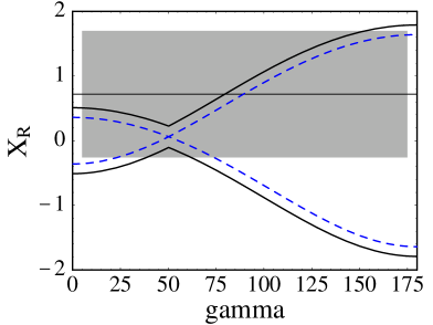
Figure 1: Upper and lower bounds on $X_{R}$ versus $|\gamma|$ (in degrees) in the SM. The dashed line shows the bounds obtained using the central values of the parameters $\bar{\varepsilon}_{3/2}$ and $\delta_{\rm EW}$. The band shows the current experimental value of $X_{R}$ with its $1\sigma$ variation.

a very good approximation, symmetric around $X_{R}=0$, we will from now on only show the upper bounds, since $X_{R}>0$ is the region favored by experiment. Also, since the bounds change little under variation of $\delta_{\rm EW}$ and $\bar{\varepsilon}_{3/2}$, we will work with the central values $\delta_{\rm EW}=0.64$ and $\bar{\varepsilon}_{3/2}=0.21$. By the time the experimental data will be sufficiently precise to perform the New Physics searches proposed in this work, the errors on these parameters are likely to be reduced by a significant amount.

Let us first discuss the case where New Physics induces arbitrary CP-violating contributions to the $B\to\pi K$ decay amplitudes, while preserving isospin symmetry. Then the only change with respect to the SM would be that the weak phase $\varphi$ may no longer be negligible. We obtain

$$R_{*}^{-1} = 1+2\bar{\varepsilon}_{3/2}\Big{[}\cos\varphi\,(\delta_{\rm EW}-\cos\gamma)\cos\phi+\sin\varphi\sin\gamma\cos(\phi-\phi_{\rho})\Big{]}$$ (29)

$$\mbox{}+\bar{\varepsilon}_{3/2}^{2}(1-2\delta_{\rm EW}\cos\gamma+\delta_{\rm EW}^{2})$$

$$\leq 1+2\bar{\varepsilon}_{3/2}\Big{[}\cos\varphi\,|\delta_{\rm EW}-\cos\gamma|+|\sin\varphi\sin\gamma|\Big{]}$$

$$\mbox{}+\bar{\varepsilon}_{3/2}^{2}(1-2\delta_{\rm EW}\cos\gamma+\delta_{\rm EW}^{2})$$

$$\leq \left(1+\bar{\varepsilon}_{3/2}\sqrt{1-2\delta_{\rm EW}\cos\gamma+\delta_{\rm EW}^{2}}\right)^{2}\,.$$

In deriving the upper bounds we have varied the strong-interaction phases $\phi$ and $\phi_{\rho}$ independently. Analogous lower bounds are obtained as previously by changing the sign of $\bar{\varepsilon}_{3/2}$. The last inequality in (29) is remarkable in that it holds for arbitrary isospin-conserving New Physics effects no matter how large they are. The corresponding bound on $|X_{R}|$ is

$$|X_{R}|\leq\sqrt{1-2\delta_{\rm EW}\cos\gamma+\delta_{\rm EW}^{2}}\leq 1+\delta_{\rm EW}\,.$$ (30)

Note that the extremal value is the same as in the SM, i.e., isospin-conserving New Physics effects cannot lead to a value of $|X_{R}|$ exceeding $1+\delta_{\rm EW}$. In the left-hand plot in Figure 2 we show the upper bound on $X_{R}$ versus $\gamma$ in the SM, and for New Physics scenarios with different values of $\varphi$. The three choices of $\varphi$ shown correspond to $|\rho|\approx 0.27$, 0.58 and 1. The gray curve shows the upper bound obtained by varying $\varphi$. We observe that isospin-conserving New Physics can enhance the value of $X_{R}$ relative to the SM, but only by a moderate amount.

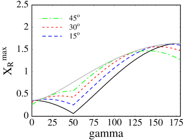
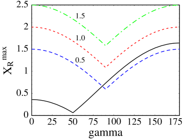
Figure 2: Upper bound on $X_{R}$ versus $|\gamma|$ for the SM (solid) and with different New Physics contributions. Left: Isospin-conserving New Physics with $|\varphi|=15^{\circ}$ (dashed), $30^{\circ}$ (short-dashed), and $45^{\circ}$ (dashed-dotted). The gray curve shows the bound (30) valid for arbitrary $\varphi$. Right: Isospin-violating but CP-conserving New Physics with $|a|=0.5$ (dashed), 1 (short-dashed), and 1.5 (dashed-dotted).

Next we consider New Physics effects that violate isospin symmetry, but we first restrict ourselves to the important subclass of models which do not contain significant new CP-violating phases. Then $\varphi$ and $b$ still vanish, and we obtain

$$R_{*}^{-1} = 1+2\bar{\varepsilon}_{3/2}\Big{[}a\cos(\phi+\phi_{a})-\cos\gamma\cos\phi\Big{]}+\bar{\varepsilon}_{3/2}^{2}(1-2a\cos\phi_{a}\cos\gamma+a^{2})$$ (31)

$$\leq \left[1+\bar{\varepsilon}_{3/2}\left(|a|+|\cos\gamma|\right)\right]^{2}+\bar{\varepsilon}_{3/2}^{2}\sin^{2}\!\gamma\,.$$

Again, a lower bound can be obtained by changing the sign of $\bar{\varepsilon}_{3/2}$. In contrast to the previous case, now the maximal value of $|X_{R}|$ is given by $1+|a|$ and thus can exceed the SM bound provided that $|a|>\delta_{\rm EW}$. This is illustrated in the right-hand plot in Figure 2, where we show the resulting upper bound on $X_{R}$ versus $\gamma$ for different values of $|a|$. In contrast with the case of isospin-conserving New Physics, even a moderate enhancement of the coefficient $a$ corresponding to a 10%–20% change in the decay amplitudes can lead to a significant increase of the upper bound on $X_{R}$.

If both isospin-violating and isospin-conserving New Physics effects are present and involve new CP-violating phases, the analysis becomes more complicated. Still, it is possible to derive from (27) a series of bounds on $R_{*}^{-1}$. We find

$$R_{*}^{-1} \leq 1+2\bar{\varepsilon}_{3/2}\Big{[}\cos\varphi\,(|a|+|\cos\gamma|)+|\sin\varphi|\,(|b|+|\sin\gamma|)\Big{]}$$ (32)

$$\mbox{}+\bar{\varepsilon}_{3/2}^{2}\Big{[}(|a|+|\cos\gamma|)^{2}+(|b|+|\sin\gamma|)^{2}\Big{]}$$

$$\leq \left[1+\bar{\varepsilon}_{3/2}\sqrt{(|a|+|\cos\gamma|)^{2}+(|b|+|\sin\gamma|)^{2}}\right]^{2}$$

$$\leq \left[1+\bar{\varepsilon}_{3/2}\left(1+\sqrt{a^{2}+b^{2}}\right)\right]^{2}\,,$$

where in the second and third steps we have eliminated $\varphi$ and $\gamma$, respectively. As before a series of lower bounds is obtained by changing the sign of $\bar{\varepsilon}_{3/2}$. The corresponding bounds on $X_{R}$ are

$$|X_{R}|\leq\sqrt{(|a|+|\cos\gamma|)^{2}+(|b|+|\sin\gamma|)^{2}}\leq 1+\sqrt{a^{2}+b^{2}}\leq\frac{2}{\bar{\varepsilon}_{3/2}}+X_{R}\,,$$ (33)

where the last inequality is relevant only in cases where $\sqrt{a^{2}+b^{2}}\gg\delta_{\rm EW}$. With the current values for $\bar{\varepsilon}_{3/2}$ and $X_{R}$, the right-hand side is less than 15 at 90% confidence level. The important point to note is that in the most general case, where $b$ and $\rho$ are nonzero, the maximal value $X_{R}$ can take is no longer restricted to occur at the endpoints $\gamma=0^{\circ}$ or $180^{\circ}$, which are disfavored by the global analysis of the unitarity triangle [37]. Rather, the maximal value $X_{R}^{\rm max}=1+\sqrt{a^{2}+b^{2}}$ now occurs at

$$|\tan\gamma|=|\rho|=\bigg{|}\frac{b}{a}\bigg{|}\,.$$ (34)

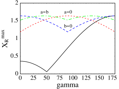
Figure 3: Upper bound on $X_{R}$ versus $|\gamma|$ for arbitrary New Physics contributions satisfying $a^{2}+b^{2}=1$. The curves correspond to $a=1$ and $b=0$ (dashed), $a=b=1/\sqrt{2}$ (dashed-dotted), and $a=0$ and $b=1$ (short-dashed). The SM bound is shown by the solid line.

The situation is illustrated in Figure 3, where we show the upper bound on $X_{R}$ for arbitrary New Physics contributions satisfying $a^{2}+b^{2}=1$, but for different values of $a$ and $b$ chosen such that the maximum occurs at the endpoints $|\gamma|=0^{\circ}$ or $180^{\circ}$ ($b=0$), at the intermediate points $|\gamma|=45^{\circ}$ or $135^{\circ}$ ($a=b$), and in the center at $|\gamma|=90^{\circ}$ ($a=0$). The corresponding values of the New Physics parameter $\rho$ required to reach the maximum are $|\rho|=0$, 1, and $\infty$ (i.e., $|\rho|\gg 1$), respectively.

The present experimental value of $X_{R}$ in (24) has too large an error to determine whether there is any deviation from the SM prediction. If $X_{R}$ turns out to be larger than 1 (i.e., only about one third of a standard deviation above its current central value), then an interpretation of this result in the SM would require a large value $|\gamma|>96^{\circ}$ (see Figure 1), which may be difficult to accommodate. This may be taken as evidence for New Physics. If $X_{R}>1.3$, one could go a step further and conclude that this New Physics must necessarily violate isospin.

3.3 New Physics effects on the determination of $\gamma$

A value of the observable $R_{*}$ which violates the SM bound (28) would be an exciting hint for new isospin-violating penguin contributions from New Physics. With the current central value of $R_{*}$ derived from CLEO data this is still a realistic possibility. However, even if a more precise measurement will give a value that is consistent with the SM bound, $B^{\pm}\to\pi K$ decays still provide an excellent testing ground for physics beyond the SM. In the SM, the weak phase $\gamma$, along with the strong-interaction phase $\phi$, can be determined up to discrete ambiguities by combining measurements of $R_{*}$ and an asymmetry $\widetilde{A}$, which is defined as a linear combination of the direct CP asymmetries in the two $B^{\pm}\to\pi K$ decay channels [8, 9]. The discrete ambiguities can be resolved using information on the strong-interaction phase $\phi$ from theoretical approaches such as the QCD factorization theorem derived in [24]. The theoretical uncertainty on the value of $\gamma$ is typically of order $10^{\circ}$. Although New Physics may not be exotic enough to lead to a violation of the general bounds derived in the previous section, it may still cause a significant shift in the extracted value of $\gamma$. This may lead to inconsistencies when the value $\gamma_{\pi K}$ extracted in $B^{\pm}\to\pi K$ decays is compared with determinations of $\gamma$ using other information.

A global fit of the unitarity triangle combining information from semileptonic $B$ decays, $B$–$\bar{B}$ mixing, CP violation in the kaon system, and mixing-induced CP violation in $B\to J/\psi\,K_{S}$ decays will provide information on $\gamma$, which in a few years will determine its value within a rather narrow range [7, 37]. Such an indirect determination could be complemented by direct measurements of $\gamma$ using, e.g., $B\to DK^{(*)}$ decays [38], or using the triangle relation $\gamma=180^{\circ}-\alpha-\beta$ combined with a measurement of $\alpha$ in $B\to\pi\pi$ or $B\to\pi\rho$ decays [7]. In our discussion below we will assume that a discrepancy between the “true” $\gamma=\mbox{arg}(V_{ub}^{*})$ and the value $\gamma_{\pi K}$ extracted in $B^{\pm}\to\pi K$ decays of more than $25^{\circ}$ will be observable after a few years of operation at the $B$ factories. This will set the benchmark for sensitivity to New Physics effects.

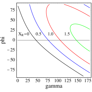
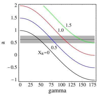
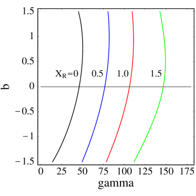
Figure 4: Contours of constant $X_{R}$ versus $\gamma$ for different New Physics parameters, assuming $\gamma>0$. In each plot one of the three parameters $\varphi$, $a$ and $b$ is varied, while the other two are kept fixed at their SM values. The horizontal lines indicate the SM results.

In order to illustrate how big an effect New Physics could have on the value of $\gamma$ extracted from $B^{\pm}\to\pi K$ decays, we assume for simplicity that the strong-interaction phase $\phi$ is small. We expect that this is indeed a good assumption, since the QCD factorization theorem of [24] predicts that $\phi=O(\alpha_{s},\Lambda/m_{b})$. In this case, a measurement of the asymmetry $\widetilde{A}$ will provide information about $\phi$ (and serve as a test of our assumption), whereas $\gamma$ is determined by $R_{*}$ alone. In the context of the SM, the solution obtained with $\cos\phi\approx 1$ is

$$\cos\gamma_{\pi K}\approx\delta_{\rm EW}-\frac{R_{*}^{-1}-1-\bar{\varepsilon}_{3/2}^{2}(1-\delta_{\rm EW}^{2})}{2\bar{\varepsilon}_{3/2}(1+\bar{\varepsilon}_{3/2}\delta_{\rm EW})}\approx\delta_{\rm EW}-\frac{R_{*}^{-1}-1}{2\bar{\varepsilon}_{3/2}}\,.$$ (35)

Given the present uncertainties in $\bar{\varepsilon}_{3/2}$ and $\delta_{\rm EW}$, this result is a good approximation to the exact solution as long as $|\phi|<25^{\circ}$. Let us now investigate how New Physics may affect the results of this extraction, neglecting, for the purpose of illustration, all strong-interaction phases. As in the previous section, we focus first on the situation where the New Physics conserves isospin symmetry. Inserting for $R_{*}^{-1}$ in (35) the expression given in (29), we obtain

$$\cos\gamma_{\pi K}=\cos(\gamma+\varphi)+\delta_{\rm EW}\,(1-\cos\varphi)+O(\bar{\varepsilon}_{3/2})\,.$$ (36)

For small values of $\varphi$, the result is simply given by $\gamma_{\pi K}\approx\gamma+\varphi$. Therefore, to have a significant shift requires having $|\varphi|>25^{\circ}$, which corresponds to rather large values $|\rho|>0.5$ and hence an $O(1)$ change in the decay amplitudes. The situation is different if the New Physics contributions violate isospin symmetry. Consider, for simplicity, the case where there are no new CP-violating phases. From (31) it then follows that

$$\cos\gamma_{\pi K}=\cos\gamma-a_{\rm NP}+O(\bar{\varepsilon}_{3/2})\,,$$ (37)

where

$$a_{\rm NP}\equiv a-\delta_{\rm EW}\,.$$ (38)

Now even a moderate New Physics contribution to the electroweak penguin coefficients can lead to a large shift in $\gamma$. In the most general case, where all New Physics contributions are present, we obtain

$$\cos\gamma_{\pi K}=\cos(\gamma+\varphi)+\delta_{\rm EW}-a\cos\varphi+b\sin\varphi+O(\bar{\varepsilon}_{3/2})\,,$$ (39)

which again allows for large shifts.

These observations are illustrated in Figure 4, where we show contours of constant $X_{R}$ versus $\gamma$ for different values of one of the parameters $\varphi$, $a$ and $b$, keeping the other two fixed to their SM values. Without loss of generality we assume that $\gamma>0$. These plots show that even moderate New Physics contributions to the parameter $a$ can induce large shifts in $\gamma$. On the other hand, small values of $\varphi$ lead to much smaller effects. Likewise, the effects induced by the parameter $b$ are much smaller. We stress that the present central value of $X_{R}\approx 0.7$ is such that negative values of $\varphi$, as well as values of $a$ less than the SM result $a\approx 0.64$, are disfavored since they would require values of $\gamma$ exceeding $100^{\circ}$, in conflict with the global analysis of the unitarity triangle [7, 37].

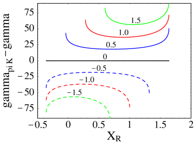
Figure 5: Difference $\gamma_{\pi K}-\gamma$ versus $X_{R}$ for different New Physics scenarios, assuming $\gamma>0$. Left: $a=\delta_{\rm EW}$, $b=0$ and $\varphi=0$, $\pm 15^{\circ}$, $\pm 30^{\circ}$, and $\pm 45^{\circ}$. Right: $\varphi=b=0$ and $a_{\rm NP}/\delta_{\rm EW}=0$, $\pm 0.5$, $\pm 1$, and $\pm 1.5$. Solid curves refer to positive values of $\varphi$ and $a_{\rm NP}$, dashed curves to negative ones.

In Figure 5, we show the difference $\gamma_{\pi K}-\gamma$ as a function of $X_{R}$ for the two cases where either $\varphi$ or $a$ are varied with respect to their SM values. The dashed curves in the plots refer to negative values of $\varphi$ or $a_{\rm NP}$, which are disfavored by the present value of $X_{R}$. This implies that isospin-conserving New Physics can only lead to moderate shifts in $\gamma$, which reach the $30^{\circ}$ level for large values $\rho=O(1)$. Isospin-violating New Physics effects, on the other hand, can induce very large shifts of $\gamma$ even if they are of moderate size. As an example, consider the case where a future, precise measurement would yield $X_{R}=1$. An interpretation of this result in the SM would imply a relatively large value $\gamma\approx 106^{\circ}$, which can be determined with a theoretical uncertainty of about $10^{\circ}$ or better [8, 9]. Imagine that all other information about the unitarity triangle favors a value of $\gamma\approx 75^{\circ}$, again with a small error. To accommodate this difference, one could either invoke a large, isospin-conserving but CP-violating New Physics contribution such that $\varphi\approx 45^{\circ}$ (corresponding to $\rho\approx 1$), or an isospin-violating electroweak penguin contribution such that $a$ is twice as large as in the SM. The first solution would imply a New Physics contribution to the decay amplitudes of order 100%, whereas the second would imply only a small contribution of less than 15%.

3.4 “Wrong kaon” decays

So far, when considering $B\to\pi K$ decays we have implicitly assumed an underlying quark transition of the form $\bar{b}\to\bar{s}q\bar{q}$, in which case the decays with a neutral kaon in the final state are $B^{+}\to\pi^{+}K^{0}$ and $B^{-}\to\pi^{-}\bar{K}^{0}$. Indeed, in the SM this is an excellent approximation, because the quark transition $\bar{b}\to\bar{d}s\bar{d}$ leading to the “wrong kaon” decays $B^{+}\to\pi^{+}\bar{K}^{0}$ and $B^{-}\to\pi^{-}K^{0}$ is highly suppressed. However, this may no longer be the case in the presence of New Physics.

In practice, only the $B^{\pm}\to\pi^{\pm}K_{S,L}$ decay rates can be measured. In particular, the CLEO result for $R_{*}$ quoted in (23) really refers to the ratio

$$R_{*}^{\rm exp}=\frac{\mbox{B}(B^{+}\to\pi^{+}K_{S})+\mbox{B}(B^{-}\to\pi^{-}K_{S})}{\mbox{B}(B^{+}\to\pi^{0}K^{+})+\mbox{B}(B^{-}\to\pi^{0}K^{-})}\equiv R_{*}\,(1+|X_{\rm wrong}|^{2})\,,$$ (40)

which differs from $R_{*}$ by the “wrong kaon” contribution

$$|X_{\rm wrong}|^{2}=\frac{\mbox{B}(B^{+}\to\pi^{+}\bar{K}^{0})+\mbox{B}(B^{-}\to\pi^{-}K^{0})}{\mbox{B}(B^{+}\to\pi^{+}K^{0})+\mbox{B}(B^{-}\to\pi^{-}\bar{K}^{0})}\,.$$ (41)

Note that the presence of this contribution could only enhance the observed value $R_{*}^{\rm exp}$ with respect to $R_{*}$. This observation, combined with the fact that $R_{*}^{\rm exp}$ is not much larger than the expected value for $R_{*}$ in the SM, allows us to put bounds on the “wrong kaon” contribution in specific New Physics models.

In analogy with (2), there are three operators entering the effective Hamiltonian for $\bar{b}\to\bar{d}s\bar{d}$ decays, which we define as

$$O_{1}^{dd} = (\bar{b}_{\alpha}d_{\alpha})_{V-A}\,(\bar{s}_{\beta}d_{\beta})_{V+A}\,,$$

$$O_{2}^{dd} = (\bar{b}_{\alpha}d_{\beta})_{V-A}\,(\bar{s}_{\beta}d_{\alpha})_{V+A}\,,$$

$$O_{3}^{dd} = (\bar{b}_{\alpha}d_{\alpha})_{V-A}\,(\bar{s}_{\beta}d_{\beta})_{V-A}\,,$$ (42)

and similarly there may be operators $\widetilde{O}_{i}^{dd}$ of opposite chirality. We denote the corresponding Wilson coefficients by $c_{i}^{dd}$ and $\widetilde{c}_{i}^{dd}$, respectively. The renormalization-group evolution of these coefficients can be read off from (2) and (2) by replacing $c_{1}^{\rm EW}\to c_{1}^{dd}$, $c_{2}^{\rm EW}\to c_{2}^{dd}$, and $c_{3,4}^{\rm EW}\to c_{3}^{dd}$. Using factorization, and normalizing the result to $\bar{\varepsilon}_{3/2}$, we find

$$X_{\rm wrong}=\frac{\bar{\varepsilon}_{3/2}}{|\lambda_{u}|}\left[\bar{c}_{3}^{dd}-\frac{2}{3}\,\kappa^{3/23}\,\bar{c}_{1}^{dd}+\frac{3\chi-1}{4}\,\kappa^{30/23}\bigg{(}\bar{c}_{2}^{dd}+\frac{1}{3}\,\bar{c}_{1}^{dd}\bigg{)}\right]\,,$$ (43)

where $\bar{c}_{i}^{dd}\equiv c_{i}^{dd}(m_{W})-\widetilde{c}_{i}^{dd}(m_{W})$. Inserting this result into (40), and performing the evolution to the scale $\mu=m_{b}$, we obtain

$$|\bar{c}_{3}^{dd}-0.26\bar{c}_{1}^{dd}+1.40\bar{c}_{2}^{dd}|\approx\frac{|\lambda_{u}|}{\bar{\varepsilon}_{3/2}}\sqrt{\frac{R_{*}^{\rm exp}}{R_{*}}-1}\,.$$ (44)

Using the current values of $\lambda_{u}$, $\bar{\varepsilon}_{3/2}$ and $R_{*}^{\rm exp}$, and taking $R_{*}>0.45$ corresponding to the smallest possible value in the SM, we find that the right-hand side is less than $5.2\times 10^{-3}$ at 90% confidence level.

4 Trojan penguins from tree-level processes

In this and the following sections, we calculate the matching conditions for the penguin coefficients $c_{i}^{q}$ and $\widetilde{c}_{i}^{q}$ in a variety of extensions of the SM with new flavor-violating couplings. We focus first on models where such couplings appear at tree level. Loop-mediated New Physics contributions will be discussed in Section 5.

4.1 Flavor-changing $Z$-boson exchange

A generic feature of extensions of the SM with extra nonsequential quarks is the presence of tree-level flavor-changing couplings of the $Z$ boson, such as a $bsZ$ vertex. A detailed discussion of such models can be found, e.g., in [40]. The relevant terms in the Lagrangian read

$${\cal L}_{\rm FCNC}=-\frac{g}{4\cos\theta_{W}}\,\sum_{i\neq j}\,\bar{d}^{i}\,[\kappa_{L}^{ij}\gamma^{\mu}(1-\gamma_{5})+\kappa_{R}^{ij}\gamma^{\mu}(1+\gamma_{5})]\,d^{j}Z_{\mu}\,,$$ (45)

where $i,j$ are generation indices. The quantities $\kappa_{L}^{bs}$ and $\kappa_{R}^{bs}$ are the two new complex parameters relevant to $b\to s$ transitions. Since the flavor-violating interactions are small (see below), the flavor-diagonal couplings of the $Z$-boson are to leading order the same as in the SM. It follows that at low energies the tree-level $Z$ exchange for the decay $\bar{b}\to\bar{s}q\bar{q}$ leads to the effective Hamiltonian

$${\cal H}_{\rm eff}=\frac{G_{F}}{\sqrt{2}}\,[\kappa_{L}^{bs}(\bar{b}s)_{V-A}+\kappa_{R}^{bs}(\bar{b}s)_{V+A}]\,\sum_{q}\,[C_{L}^{q}(\bar{q}q)_{V-A}+C_{R}^{q}(\bar{q}q)_{V+A}]\,,$$ (46)

where

$$C_{L}^{u} = \phantom{-}\frac{1}{2}-\frac{2}{3}\sin^{2}\!\theta_{W}\,,\qquad C_{R}^{u}=-\frac{2}{3}\sin^{2}\!\theta_{W}\,,$$

$$C_{L}^{d} = -\frac{1}{2}+\frac{1}{3}\sin^{2}\!\theta_{W}\,,\qquad C_{R}^{d}=\phantom{-}\frac{1}{3}\sin^{2}\!\theta_{W}\,.$$ (47)

It is straightforward to match this result with the generic form of the penguin terms in the effective Hamiltonian, and to deduce the corresponding values of the Wilson coefficients. The nonvanishing coefficients at the matching scale are $c_{1}^{q}=\kappa_{L}^{bs}\,C_{R}^{q}$, $c_{3}^{q}=\kappa_{L}^{bs}\,C_{L}^{q}$, $\widetilde{c}_{1}^{q}=\kappa_{R}^{bs}\,C_{L}^{q}$, and $\widetilde{c}_{3}^{q}=\kappa_{R}^{bs}\,C_{R}^{q}$. In the notation of (7), this implies

$$c_{3}^{\rm QCD}=-\frac{\kappa_{L}^{bs}}{6}\,,\qquad\widetilde{c}_{1}^{\rm QCD}=-\frac{\kappa_{R}^{bs}}{6}\,,\qquad c_{1}^{\rm QCD}=\widetilde{c}_{3}^{\rm QCD}=0\,,$$ (48)

as well as

$$c_{1}^{\rm EW} = -\kappa_{L}^{bs}\sin^{2}\!\theta_{W}\,,\qquad c_{3}^{\rm EW}=\phantom{-}\kappa_{L}^{bs}\cos^{2}\!\theta_{W}\,,$$

$$\widetilde{c}_{1}^{\rm EW} = \phantom{-}\kappa_{R}^{bs}\cos^{2}\!\theta_{W}\,,\qquad\widetilde{c}_{3}^{\rm EW}=-\kappa_{R}^{bs}\sin^{2}\!\theta_{W}\,.$$ (49)

These electroweak penguin coefficients would be of the same order as the SM result for $c_{3}^{\rm EW}$ in (2) if $|\kappa_{L,R}^{bs}|\approx 5\times 10^{-4}$ which, as we will see below, is consistent with experimental bounds. Inserting these results into (17) and using $|\lambda_{u}|\approx 7.5\times 10^{-4}$ yields

$$a_{\rm NP}+ib\approx-1.1\times 10^{3}\,(\kappa_{L}^{bs}+0.51\kappa_{R}^{bs})\,.$$ (50)

We stress that the simple model considered here is a prototype of New Physics models in which the electroweak penguin coefficients $c_{i}^{\rm EW}$ and $\widetilde{c}_{i}^{\rm EW}$ are not suppressed relative to the QCD penguin coefficients $c_{i}^{\rm QCD}$ and $\widetilde{c}_{i}^{\rm QCD}$. This property is in contrast with the SM, where electroweak penguins are suppressed by small gauge couplings.

At present, the strongest constraints on $\kappa_{L}^{bs}$ and $\kappa_{R}^{bs}$ follow from the experimental bound on the $B\to X_{s}\,e^{+}e^{-}$ decay rate. Since this bound lies far above the SM prediction for this process, we can neglect the SM contribution and write the effective Hamiltonian for this process as

$${\cal H}_{\rm eff}=\frac{G_{F}}{\sqrt{2}}\,[\kappa_{L}^{bs}(\bar{b}s)_{V-A}+\kappa_{R}^{bs}(\bar{b}s)_{V+A}]\left[C_{L}^{e}\,(\bar{e}e)_{V-A}+C_{R}^{e}\,(\bar{e}e)_{V+A}\right]\,,$$ (51)

where

$$C_{L}^{e}=-\frac{1}{2}+\sin^{2}\!\theta_{W}\,,\qquad C_{R}^{e}=\sin^{2}\!\theta_{W}\,.$$ (52)

It is convenient to normalize the result for the $B\to X_{s}\,e^{+}e^{-}$ decay rate to the semileptonic rate. Then many common factors cancel, and we obtain

$$\frac{\Gamma(B\to X_{s}\,e^{+}e^{-})}{\Gamma(B\to X_{c}\,e^{-}\bar{\nu}_{e})}=\frac{|\kappa_{L}^{bs}|^{2}+|\kappa_{R}^{bs}|^{2}}{f(m_{c}/m_{b})\,|V_{cb}|^{2}}\left[(C_{L}^{e})^{2}+(C_{R}^{e})^{2}\right]\approx 157\left(|\kappa_{L}^{bs}|^{2}+|\kappa_{R}^{bs}|^{2}\right)\,,$$ (53)

where we have used $|V_{cb}|\approx 0.04$, and $f(m_{c}/m_{b})\approx 0.5$ for the phase-space factor in the semileptonic decay. Using the upper bound $\mbox{B}(B\to X_{s}\,e^{+}e^{-})<5.7\times 10^{-5}$ together with $\mbox{B}(B\to X_{c}\,e^{-}\bar{\nu}_{e})=0.105$ [41] yields

$$\sqrt{|\kappa_{L}^{bs}|^{2}+|\kappa_{R}^{bs}|^{2}}<1.9\times 10^{-3}\,.$$ (54)

Combining this result with (50), we obtain the upper bound

$$\sqrt{a_{\rm NP}^{2}+b^{2}}<2.0\,,$$ (55)

which may be compared with the SM value $a\approx 0.64$. It follows that tree-level $Z$ exchange with new flavor-violating couplings can yield isospin-violating electroweak penguin effects that are up to a factor 3 larger than in the SM.

For completeness, we also mention the resulting bound on the New Physics parameter $\rho$. Neglecting renormalization-group effects, we obtain from (20) the estimate

$$\frac{\rho}{\sqrt{1+\rho^{2}}}\approx 29\,\Big{[}0.8\,\mbox{Im}\,\kappa_{L}^{bs}+\mbox{Im}\,\kappa_{R}^{bs}\Big{]}\quad\Rightarrow\quad|\rho|<0.05\,,\quad|\varphi|<3^{\circ}\,,$$ (56)

indicating that in this model there is no room for large values of $\rho$.

4.2 Extended gauge models with a $Z^{\prime}$ boson

A new neutral boson $Z^{\prime}$ with tree-level flavor-changing couplings to quarks is a generic property of many models with an extended gauge group. The analysis of electroweak penguins in such models is very similar to the flavor-changing tree-level $Z$ exchange discussed above. For simplicity, we assume no significant mixing between the $Z$ and $Z^{\prime}$ bosons. Then the effective Hamiltonian is a simple generalization of (46), i.e.

$${\cal H}_{\rm eff} = \frac{g_{U(1)^{\prime}}^{2}}{m_{Z^{\prime}}^{2}}[\kappa_{L}^{\prime bs}(\bar{b}s)_{V-A}+\kappa_{R}^{\prime bs}(\bar{b}s)_{V+A}]\,\sum_{q}\,[C_{L}^{q}(\bar{q}q)_{V-A}+C_{R}^{q}(\bar{q}q)_{V+A}]\,,$$ (57)

where $C_{L,R}^{q}$ now denote the charges of the quarks under the new U$(1)^{\prime}$ group. Introducing the ratio

$$\xi=\frac{g_{{\rm U}(1)^{\prime}}^{2}}{g^{2}}\,\frac{m_{W}^{2}}{m_{Z^{\prime}}^{2}}\,,$$ (58)

and taking into account that, since we neglect $Z$–$Z^{\prime}$ mixing, the $Z^{\prime}$ charges are the same for all left-handed fields (in particular, $C_{L}^{u}=C_{L}^{d}$), we find

$$c_{1}^{\rm QCD} = \xi\kappa_{L}^{\prime bs}\,\frac{C_{R}^{u}+2C_{R}^{d}}{3}\,,\qquad c_{3}^{\rm QCD}=\xi\kappa_{L}^{\prime bs}C_{L}^{q}\,,$$

$$\widetilde{c}_{1}^{\rm QCD} = \xi\kappa_{R}^{\prime bs}C_{L}^{q}\,,\qquad\widetilde{c}_{3}^{\rm QCD}=\xi\kappa_{R}^{\prime bs}\,\frac{C_{R}^{u}+2C_{R}^{d}}{3}\,,$$ (59)

and

$$c_{1}^{\rm EW}=\xi\kappa_{L}^{\prime bs}(C_{R}^{u}-C_{R}^{d})\,,\qquad\widetilde{c}_{3}^{\rm EW}=\xi\kappa_{R}^{\prime bs}(C_{R}^{u}-C_{R}^{d})\,,\qquad c_{3}^{\rm EW}=\widetilde{c}_{1}^{\rm EW}=0\,.$$ (60)

Inserting these results into (17) gives

$$a_{\rm NP}+ib\approx\frac{\xi(C_{R}^{u}-C_{R}^{d})}{|\lambda_{u}|}\,(\kappa_{R}^{\prime bs}+0.26\kappa_{L}^{\prime bs})\,.$$ (61)

The allowed range for the relevant parameters in $Z^{\prime}$ extensions of the SM is largely model dependent. For example, the bounds derived from the upper limit on the $B\to X_{s}\,l^{+}l^{-}$ branching ratio depend on the lepton charges under the new U$(1)^{\prime}$ gauge group. In the so-called “leptophobic” $Z^{\prime}$ models these charges are arranged so as to vanish or be very small [42]. Therefore, in general the contributions of the $Z^{\prime}$ couplings to the electroweak penguin operators can be arbitrarily large. In fact, the best model-independent bound on these couplings follows from the second inequality in (33), which implies

$$|\xi(C_{R}^{u}-C_{R}^{d})|\,|\kappa_{R}^{\prime bs}+0.26\kappa_{L}^{\prime bs}|<0.01\,,$$ (62)

where we have neglected the small SM contribution. Furthermore, assuming $C_{L,R}^{q}=O(1)$ and no cancellations, the bound (22) gives $|\xi\,\mbox{Im}\,\kappa_{L,R}^{\prime bs}|<O(10^{-2})$. Turning these observations around, we conclude that in extended gauge models with flavor-changing $Z^{\prime}$ couplings such that $\xi\kappa_{L,R}^{\prime bs}=O(10^{-2})$ there can be very large New Physics effects in $B\to\pi K$ decays.

4.3 SUSY models with R-parity violation

In SUSY models with broken R-parity extra trilinear terms are allowed in the superpotential, some of which can give rise to a large enhancement of the electroweak penguin coefficients. Denoting by $L_{L}^{i}$, $Q_{L}^{i}$, $u_{R}^{i}$ and $d_{R}^{i}$ the chiral superfields containing, respectively, the left-handed lepton and quark doublets, and the right-handed up- and down-type quark singlets of the $i$-th generation, these terms read

$$W=\lambda^{\prime}_{ijk}\,L_{L}^{i}\,Q_{L}^{j}\,\bar{d}_{R}^{k}+\lambda^{\prime\prime}_{ijk}\,\bar{u}_{R}^{i}\,\bar{d}_{R}^{j}\,\bar{d}_{R}^{k}\,.$$ (63)

At low energies, slepton and squark exchange can generate local penguin operators. The most general case has been treated in [18]. For simplicity, we neglect left-right sfermion mixing, which is a small effect and does not generate new operators. We then find for the coefficients of the various penguin operators

$$\widetilde{c}_{2}^{u}=\sum_{i=1}^{3}\frac{\lambda_{i12}^{\prime*}\lambda^{\prime}_{i13}}{4\sqrt{2}G_{F}m_{\tilde{e}_{iL}}^{2}}\,,\qquad-\widetilde{c}_{3}^{u}=\widetilde{c}_{4}^{u}=\frac{\lambda_{113}^{\prime\prime*}\lambda^{\prime\prime}_{112}}{2\sqrt{2}G_{F}m_{\tilde{d}_{1R}}^{2}}\,,$$ (64)

and

$$c_{2}^{d} = \sum_{i=1}^{3}\frac{\lambda_{i31}^{\prime*}\lambda^{\prime}_{i21}}{4\sqrt{2}G_{F}m_{\tilde{\nu}_{i}}^{2}}\,,\qquad c_{6}^{d}=\sum_{i=1}^{3}\frac{\lambda_{i32}^{\prime*}\lambda^{\prime}_{i11}}{4\sqrt{2}G_{F}m_{\tilde{\nu}_{i}}^{2}}\,,$$

$$\widetilde{c}_{2}^{d} = \sum_{i=1}^{3}\frac{\lambda_{i12}^{\prime*}\lambda^{\prime}_{i13}}{4\sqrt{2}G_{F}m_{\tilde{\nu}_{i}}^{2}}\,,\qquad\widetilde{c}_{6}^{d}=\sum_{i=1}^{3}\frac{\lambda_{i11}^{\prime*}\lambda^{\prime}_{i23}}{4\sqrt{2}G_{F}m_{\tilde{\nu}_{i}}^{2}}\,,$$

$$-\widetilde{c}_{3}^{d} = \widetilde{c}_{4}^{d}=\sum_{i=1}^{3}\frac{\lambda_{i13}^{\prime\prime*}\lambda^{\prime\prime}_{i12}}{2\sqrt{2}G_{F}m_{\tilde{u}_{iR}}^{2}}\,.$$ (65)

Previous authors have investigated bounds on some of these R-parity violating couplings in the context of nonleptonic $B$ decays [43, 44]. However, in these studies model-dependent predictions for the overall penguin amplitude $P$ in (3.1) are employed. The only significant bound which has an impact on our analysis comes from a combination of constraints derived from limits on double nucleon decay into two kaons and neutron–antineutron oscillations, yielding $|\lambda_{113}^{\prime\prime*}\lambda^{\prime\prime}_{112}|<10^{-9}$ [43]. Therefore, is it safe to neglect $\widetilde{c}_{3}^{u}$ and $\widetilde{c}_{4}^{u}$.

Not all of the above coefficients contribute to the isospin-violating terms parametrized by $a$ and $b$. Up to a small SU(2)_L breaking in the slepton and sneutrino masses we find $\widetilde{c}_{2}^{u}=\widetilde{c}_{2}^{d}$, and thus $\widetilde{c}_{2}^{\rm EW}\approx 0$. Moreover, in (17) only the sum $\bar{c}_{3}^{\rm EW}+\bar{c}_{4}^{\rm EW}$ contributes, which vanishes since $\widetilde{c}_{3}^{q}=-\widetilde{c}_{4}^{q}$. It follows that

$$a_{\rm NP}+ib\approx 2.83\times 10^{3}\,\sum_{i=1}^{3}\,\frac{(100\,\mbox{GeV})^{2}}{m_{\tilde{\nu}_{i}}^{2}}\,\Big{(}{\lambda_{i31}^{\prime*}\lambda^{\prime}_{i21}}+\lambda_{i32}^{\prime*}\lambda^{\prime}_{i11}-\lambda_{i11}^{\prime*}\lambda^{\prime}_{i23}\Big{)}\,.$$ (66)

The result for the parameter $\rho$ is more complicated. Setting for simplicity all sfermion masses equal, we find from (20)

$$\frac{\rho}{\sqrt{1+\rho^{2}}} \approx 106\,\frac{(100\,\mbox{GeV})^{2}}{m_{\tilde{f}}^{2}}$$ (67)

$$\times \sum_{i=1}^{3}\,\mbox{Im}\Big{[}4\lambda_{i13}^{\prime\prime*}\lambda^{\prime\prime}_{i12}+3\chi(\lambda_{i12}^{\prime*}\lambda^{\prime}_{i13}-\lambda_{i31}^{\prime*}\lambda^{\prime}_{i21})+\lambda_{i32}^{\prime*}\lambda^{\prime}_{i11}-\lambda_{i11}^{\prime*}\lambda^{\prime}_{i23}\Big{]}\,.\qquad$$

Using the results derived in Section 3, we can obtain bounds on several of the R-parity violating couplings. Assuming that only one combination of couplings is dominant, neglecting the SM contribution, and using a common sfermion reference mass of $100\,$GeV, we find from (33) that at 90% confidence level

$$\Big{|}\sum_{i=1}^{3}\,\lambda_{i31}^{\prime*}\lambda^{\prime}_{i21}\Big{|} < 4.9\times 10^{-3}\,,$$

$$\Big{|}\sum_{i=1}^{3}\,\lambda_{i32}^{\prime*}\lambda^{\prime}_{i11}|\Big{|} < 4.9\times 10^{-3}\,,$$

$$\Big{|}\sum_{i=1}^{3}\,\lambda_{i11}^{\prime*}\lambda^{\prime}_{i23}|\Big{|} < 4.9\times 10^{-3}\,.$$ (68)

In addition, from (22) we obtain

$$\Big{|}\sum_{i=1}^{3}\,\mbox{Im}\,(\lambda_{i13}^{\prime\prime*}\lambda^{\prime\prime}_{i12})\Big{|} < 3.7\times 10^{-3}\,,$$

$$\Big{|}\sum_{i=1}^{3}\,\mbox{Im}\,(\lambda_{i31}^{\prime*}\lambda^{\prime}_{i21})\Big{|} < 4.1\times 10^{-3}\,,$$

$$\Big{|}\sum_{i=1}^{3}\,\mbox{Im}\,(\lambda_{i12}^{\prime*}\lambda^{\prime}_{i13})\Big{|} < 4.1\times 10^{-3}\,,$$ (69)

where we do not present bounds on the imaginary parts of couplings which are weaker than the corresponding bounds on the absolute values in (4.3).

It is interesting that SUSY models with R-parity violation provide an example of scenarios in which $\bar{b}\to\bar{d}s\bar{d}$ transitions may not be suppressed relative to $\bar{b}\to\bar{s}d\bar{d}$ transitions. As pointed out in Section 3, this can lead to potentially large “wrong kaon” decays of the type $B^{+}\to\pi^{+}\bar{K}^{0}$ and $B^{-}\to\pi^{-}K^{0}$. In the model considered here, the only nonvanishing coefficients are

$$c_{2}^{dd}=\sum_{i=1}^{3}\frac{\lambda_{i31}^{\prime*}\lambda^{\prime}_{i12}}{4\sqrt{2}G_{F}m_{\tilde{\nu}_{i}}^{2}}\,,\qquad\widetilde{c}_{2}^{dd}=\sum_{i=1}^{3}\frac{\lambda_{i21}^{\prime*}\lambda^{\prime}_{i13}}{4\sqrt{2}G_{F}m_{\tilde{\nu}_{i}}^{2}}\,.$$ (70)

The result (44) can be used to obtain the bounds

$$|\lambda_{i31}^{\prime*}\lambda^{\prime}_{i12}|<3.4\times 10^{-3}\,,\qquad|\lambda_{i21}^{\prime*}\lambda^{\prime}_{i13}|<3.4\times 10^{-3}\,,$$ (71)

again at 90% confidence level.

Our bounds in (4.3) and (4.3) are stronger than the ones discussed in the literature [43, 44] and refer to a larger number of $R$-parity violating couplings. Most importantly, however, they are affected by much smaller hadronic uncertainties. The bounds in (71), on the other hand, are weaker than constraints derived from $B$–$\bar{B}$ and $K$–$\bar{K}$ mixing [45].

5 Trojan penguins from loop processes

Having considered in the previous section some specific models with tree-level FCNC couplings, we now explore extensions of the SM in which new contributions to the electroweak and QCD penguin operators arise at one-loop order. In particular, we study in detail the structure of electroweak penguins in SUSY models, where isospin-violating $\bar{b}\to\bar{s}q\bar{q}$ transitions can arise due to strong-interaction gluino box diagrams. This provides another realization of models in which electroweak penguins are not suppressed relative to QCD penguins. For completeness, we also discuss two-Higgs–doublet models and models with anomalous gauge-boson couplings. They are simple since there are no new CP-violating phases, so only the parameter $a$ can receive a New Physics contribution. However, there is no parametrical enhancement of the electroweak penguins relative to the SM, and thus the New Physics contributions tend to be small.

5.1 SUSY models

In SUSY extensions of the SM with conserved R-parity, the potentially most important contributions to the Wilson coefficients of the penguin operators in the effective Hamiltonian (6) arise from strong-interaction penguin and box diagrams with gluino–squark loops. They can contribute to FCNC processes because the gluinos have flavor-changing couplings to the quark and squark mass eigenstates. Provided there is a significant mass splitting between the right-handed up and down squarks, gluino box diagrams are also the most important source of isospin violation in SUSY models [15]. The corresponding contributions to the electroweak penguin coefficients are then much more important than other SUSY contributions from photon or $Z$ penguins usually discussed in the literature. In fact, in such a scenario SUSY contributions to the coefficients of the electroweak and QCD penguin operators are of the same order and scale like $\alpha_{s}^{2}/m_{\rm SUSY}^{2}$, where $m_{\rm SUSY}$ is a generic mass of the superparticles. Whereas the QCD penguin contributions are typically smaller than in the SM, the electroweak penguin contributions can be important, since their scaling relative to the SM coefficients is controlled by the ratio $(\alpha_{s}/\alpha)(m_{W}^{2}/m_{\rm SUSY}^{2})\sim 1$. In our analysis we will consider only these potentially large gluino box and penguin contributions and neglect a multitude of other SUSY diagrams, which are parametrically suppressed by small electroweak gauge couplings. The latter include photon or $Z$ penguins with gluino–squark, chargino–squark, neutralino–squark, or charged-Higgs–quark loops, and various box diagrams containing at least one chargino or neutralino. We have calculated all of these diagrams and, for generic regions in SUSY parameter space, have found their contributions to be largely suppressed relative to the pure gluino diagrams.

Large SUSY contributions to the penguin operators via gluino loops require near maximal mixing between the strange and bottom squarks, so that the squark mass-insertion approximation is not valid. We therefore present our results using the general vertex-mixing method, summing over diagrams with different squark mass-eigenstates in the loops [46, 47]. We denote by $\Gamma^{D_{L}}$ the rotation matrices relating the left-handed down-squark interaction states in the quark mass-eigenbasis, $\tilde{q}_{L}^{I}$ ($q=d,s,b$), to the squark mass eigenstates, $\tilde{d}_{i}$ ($i=1,\dots,6$), such that $\tilde{q}_{L}^{I}=(\Gamma^{D_{L}}_{iq})^{*}\,\tilde{d}_{i}$, with obvious generalizations for the up- and right-handed squarks. In addition, $x_{\tilde{q}_{i}\tilde{g}}\equiv m_{\tilde{q}_{i}}^{2}/m_{\tilde{g}}^{2}$, where $m_{\tilde{q}_{i}}$ is the mass of the $i$-th down ($q=d$) or up ($q=u$) squark mass eigenstate. In the operator basis of (2), we obtain for the gluino box contributions to the Wilson coefficients at the SUSY matching scale

$$c_{1,{\rm box}}^{u} = \frac{\alpha_{s}^{2}}{2\sqrt{2}G_{F}m_{\tilde{g}}^{2}}\left(\Gamma^{D_{L}}_{ib}\right)^{*}\Gamma^{D_{L}}_{is}\left(\Gamma^{U_{R}}_{ju}\right)^{*}\Gamma^{U_{R}}_{ju}\left[\frac{1}{18}\,F(x_{\tilde{d}_{i}\tilde{g}},x_{\tilde{u}_{j}\tilde{g}})-\frac{5}{18}\,G(x_{\tilde{d}_{i}\tilde{g}},x_{\tilde{u}_{j}\tilde{g}})\right],$$

$$c_{1,{\rm box}}^{d} = \frac{\alpha_{s}^{2}}{2\sqrt{2}G_{F}m_{\tilde{g}}^{2}}\left(\Gamma^{D_{L}}_{ib}\right)^{*}\Gamma^{D_{L}}_{is}\left(\Gamma^{D_{R}}_{jd}\right)^{*}\Gamma^{D_{R}}_{jd}\left[\frac{1}{18}\,F(x_{\tilde{d}_{i}\tilde{g}},x_{\tilde{d}_{j}\tilde{g}})-\frac{5}{18}\,G(x_{\tilde{d}_{i}\tilde{g}},x_{\tilde{d}_{j}\tilde{g}})\right],$$

$$c_{2,{\rm box}}^{u} = \frac{\alpha_{s}^{2}}{2\sqrt{2}G_{F}m_{\tilde{g}}^{2}}\left(\Gamma^{D_{L}}_{ib}\right)^{*}\Gamma^{D_{L}}_{is}\left(\Gamma^{U_{R}}_{ju}\right)^{*}\Gamma^{U_{R}}_{ju}\left[\frac{7}{6}\,F(x_{\tilde{d}_{i}\tilde{g}},x_{\tilde{u}_{j}\tilde{g}})+\frac{1}{6}\,G(x_{\tilde{d}_{i}\tilde{g}},x_{\tilde{u}_{j}\tilde{g}})\right],$$

$$c_{2,{\rm box}}^{d} = \frac{\alpha_{s}^{2}}{2\sqrt{2}G_{F}m_{\tilde{g}}^{2}}\left(\Gamma^{D_{L}}_{ib}\right)^{*}\Gamma^{D_{L}}_{is}\left(\Gamma^{D_{R}}_{jd}\right)^{*}\Gamma^{D_{R}}_{jd}\left[\frac{7}{6}\,F(x_{\tilde{d}_{i}\tilde{g}},x_{\tilde{d}_{j}\tilde{g}})+\frac{1}{6}\,G(x_{\tilde{d}_{i}\tilde{g}},x_{\tilde{d}_{j}\tilde{g}})\right],$$

$$c_{3,{\rm box}}^{u} = \frac{\alpha_{s}^{2}}{2\sqrt{2}G_{F}m_{\tilde{g}}^{2}}\left(\Gamma^{D_{L}}_{ib}\right)^{*}\Gamma^{D_{L}}_{is}\left(\Gamma^{U_{L}}_{ju}\right)^{*}\Gamma^{U_{L}}_{ju}\left[-\frac{5}{9}\,F(x_{\tilde{d}_{i}\tilde{g}},x_{\tilde{u}_{j}\tilde{g}})+\frac{1}{36}\,G(x_{\tilde{d}_{i}\tilde{g}},x_{\tilde{u}_{j}\tilde{g}})\right],$$

$$c_{3,{\rm box}}^{d} = \frac{\alpha_{s}^{2}}{2\sqrt{2}G_{F}m_{\tilde{g}}^{2}}\Bigg{\{}\left(\Gamma^{D_{L}}_{ib}\right)^{*}\Gamma^{D_{L}}_{is}\left(\Gamma^{D_{L}}_{jd}\right)^{*}\Gamma^{D_{L}}_{jd}\left[-\frac{5}{9}\,F(x_{\tilde{d}_{i}\tilde{g}},x_{\tilde{d}_{j}\tilde{g}})+\frac{1}{36}\,G(x_{\tilde{d}_{i}\tilde{g}},x_{\tilde{d}_{j}\tilde{g}})\right]$$

$$\hskip 51.21504pt\mbox{}+\left(\Gamma^{D_{L}}_{ib}\right)^{*}\Gamma^{D_{L}}_{js}\left(\Gamma^{D_{L}}_{jd}\right)^{*}\Gamma^{D_{L}}_{id}\left[\frac{1}{3}\,F(x_{\tilde{d}_{i}\tilde{g}},x_{\tilde{d}_{j}\tilde{g}})-\frac{7}{12}\,G(x_{\tilde{d}_{i}\tilde{g}},x_{\tilde{d}_{j}\tilde{g}})\right]\Bigg{\}},$$

$$c_{4,{\rm box}}^{u} = \frac{\alpha_{s}^{2}}{2\sqrt{2}G_{F}m_{\tilde{g}}^{2}}\left(\Gamma^{D_{L}}_{ib}\right)^{*}\Gamma^{D_{L}}_{is}\left(\Gamma^{U_{L}}_{ju}\right)^{*}\Gamma^{U_{L}}_{ju}\left[\frac{1}{3}\,F(x_{\tilde{d}_{i}\tilde{g}},x_{\tilde{u}_{j}\tilde{g}})-\frac{7}{12}\,G(x_{\tilde{d}_{i}\tilde{g}},x_{\tilde{u}_{j}\tilde{g}})\right],$$

$$c_{4,{\rm box}}^{d} = \frac{\alpha_{s}^{2}}{2\sqrt{2}G_{F}m_{\tilde{g}}^{2}}\Bigg{\{}\left(\Gamma^{D_{L}}_{ib}\right)^{*}\Gamma^{D_{L}}_{is}\left(\Gamma^{D_{L}}_{jd}\right)^{*}\Gamma^{D_{L}}_{jd}\left[\frac{1}{3}\,F(x_{\tilde{d}_{i}\tilde{g}},x_{\tilde{d}_{j}\tilde{g}})-\frac{7}{12}\,G(x_{\tilde{d}_{i}\tilde{g}},x_{\tilde{d}_{j}\tilde{g}})\right]$$

$$\hskip 51.21504pt\mbox{}+\left(\Gamma^{D_{L}}_{ib}\right)^{*}\Gamma^{D_{L}}_{js}\left(\Gamma^{D_{L}}_{jd}\right)^{*}\Gamma^{D_{L}}_{id}\left[-\frac{5}{9}\,F(x_{\tilde{d}_{i}\tilde{g}},x_{\tilde{d}_{j}\tilde{g}})+\frac{1}{36}\,G(x_{\tilde{d}_{i}\tilde{g}},x_{\tilde{d}_{j}\tilde{g}})\right]\Bigg{\}},$$

$$c_{5,{\rm box}}^{d} = \frac{\alpha_{s}^{2}}{2\sqrt{2}G_{F}m_{\tilde{g}}^{2}}\left(\Gamma^{D_{L}}_{ib}\right)^{*}\Gamma^{D_{R}}_{js}\left(\Gamma^{D_{R}}_{jd}\right)^{*}\Gamma^{D_{L}}_{id}\left[\frac{1}{18}\,F(x_{\tilde{d}_{i}\tilde{g}},x_{\tilde{d}_{j}\tilde{g}})-\frac{5}{18}\,G(x_{\tilde{d}_{i}\tilde{g}},x_{\tilde{d}_{j}\tilde{g}})\right],$$

$$c_{6,{\rm box}}^{d} = \frac{\alpha_{s}^{2}}{2\sqrt{2}G_{F}m_{\tilde{g}}^{2}}\left(\Gamma^{D_{L}}_{ib}\right)^{*}\Gamma^{D_{R}}_{js}\left(\Gamma^{D_{R}}_{jd}\right)^{*}\Gamma^{D_{L}}_{id}\left[\frac{7}{6}\,F(x_{\tilde{d}_{i}\tilde{g}},x_{\tilde{d}_{j}\tilde{g}})+\frac{1}{6}\,G(x_{\tilde{d}_{i}\tilde{g}},x_{\tilde{d}_{j}\tilde{g}})\right],$$ (72)

where repeated indices are summed over, and $c_{5,{\rm box}}^{u}=c_{6,{\rm box}}^{u}=0$. The functions $F(x,y)$ and $G(x,y)$ are given by [46, 47]

$$F(x,y) = -\frac{x\ln x}{(x-y)(x-1)^{2}}-\frac{y\ln y}{(y-x)(y-1)^{2}}-\frac{1}{(x-1)(y-1)}\,,$$

$$G(x,y) = \frac{x^{2}\ln x}{(x-y)(x-1)^{2}}+\frac{y^{2}\ln y}{(y-x)(y-1)^{2}}+\frac{1}{(x-1)(y-1)}\,.$$ (73)

The corresponding expressions for the coefficients $\widetilde{c}_{i}^{q}$ of the opposite-chirality operators are obtained via the exchange $L\leftrightarrow R$ in the expressions for $c_{i}^{q}$. In practice, $c_{5,{\rm box}}^{d}$, $c_{6,{\rm box}}^{d}$ and the second terms in $c_{3,{\rm box}}^{d}$, $c_{4,{\rm box}}^{d}$ (as well as the corresponding terms in the coefficients of the opposite-chirality operators) can be neglected due to $B_{d}$–$\bar{B}_{d}$ and $K$–$\bar{K}$ mixing constraints on the off-diagonal (1-3) and (1-2) entries of the $\Gamma^{D_{L}}$ and $\Gamma^{D_{R}}$ matrices. Gluino box diagrams which in the mass-insertion approximation would contain left–right squark-mass insertions can also be neglected and have not been included in (5.1). Specifically, these graphs would contain the mass insertions $\delta m^{2}_{\tilde{s}_{L}\tilde{b}_{R}}$, $\delta m^{2}_{\tilde{s}_{R}\tilde{b}_{L}}$, $\delta m^{2}_{\tilde{d}_{L}\tilde{b}_{R}}$ or $\delta m^{2}_{\tilde{d}_{R}\tilde{b}_{L}}$, whose magnitudes are tightly constrained by the experimental value of the $B\to X_{s,d}\,\gamma$ branching ratio [48]. Further suppression of such graphs can be expected on theoretical grounds since the remaining left–right squark-mass insertions they would contain are suppressed by light quark masses in general supergravity theories [49, 50] and in SUSY theories of flavor [51, 52, 53].

In addition to the box contributions, the QCD penguin coefficients also receive contributions from gluon penguin diagrams containing gluino–squark loops. These are given at the SUSY matching scale by [54, 55]

$$c_{1,{\rm peng}}^{q} = c_{3,{\rm peng}}^{q}=-\frac{c_{2,{\rm peng}}^{q}}{3}=-\frac{c_{4,{\rm peng}}^{q}}{3}$$ (74)

$$= \frac{\alpha_{s}^{2}}{2\sqrt{2}G_{F}m_{\tilde{g}}^{2}}\left(\Gamma^{D_{L}}_{ib}\right)^{*}\Gamma^{D_{L}}_{is}\left[\frac{1}{2}\,A(x_{\tilde{d}_{i}\tilde{g}})+\frac{2}{9}\,B(x_{\tilde{d}_{i}\tilde{g}})\right],$$

where

$$A(x) = \frac{1}{2(1-x)}+\frac{(1+2x)\ln x}{6(1-x)^{2}}\,,$$

$$B(x) = -\frac{11-7x+2x^{2}}{18(1-x)^{3}}-\frac{\ln x}{3(1-x)^{4}}\,.$$ (75)

The opposite-chirality contributions are again obtained via the substitution $L\rightarrow R$.

FCNC constraints on the off-diagonal entries of the squark mass matrix allow for a simple parametrization of the gluino box and penguin contributions to $\bar{b}\to\bar{s}u\bar{u}$ and $\bar{b}\to\bar{s}d\bar{d}$ transitions, up to small corrections which have a negligible impact on the resulting Wilson coefficients. Let us first consider the down-squark sector. Constraints from $B_{d}$–$\bar{B}_{d}$ and $K$–$\bar{K}$ mixing imply that, to good approximation, the down squark is decoupled from the strange and bottom squarks. We also neglect the left–right down-squark submatrix, since even in the most general case of supergravity theories with arbitrary Kähler potential its entries are much smaller than the typical squark-mass squared [49, 50], and in SUSY theories of flavor its entries are even more suppressed [53]. The above simplifications essentially give three “left-handed” and three “right-handed” down-squark mass eigenstates, obtained by diagonalizing the left–left and right–right squark submatrices. Specifically, in the physical down-quark basis $(d_{L},s_{L},b_{L})$ the left–left submatrix takes the form

$$M_{d,LL}^{2}\simeq\left(\begin{array}[]{ccc}m_{11}^{2}&0&0\\ 0&m_{22}^{2}&m^{2}_{23}\\ 0&(m_{23}^{2})^{*}&m_{33}^{2}\end{array}\right)\,.$$ (76)

Let us denote the left-handed mass eigenstates by $\tilde{q}_{L}$ ($q=d,s,b$) and their masses by $m_{\tilde{q}_{L}}^{2}$, making the identification $m_{\tilde{d}_{L}}^{2}=m_{11}^{2}$. Then the left-handed squark mass-eigenstates take the form

$$\tilde{d}_{L}\equiv\tilde{d}_{1}=\left(\begin{array}[]{c}1\\ 0\\ 0\end{array}\right)\,,\quad\tilde{s}_{L}\equiv\tilde{d}_{2}=\left(\begin{array}[]{c}0\\ \cos\theta_{L}\\ -\sin\theta_{L}\,e^{-i\delta_{L}}\end{array}\right)\,,\quad\tilde{b}_{L}\equiv\tilde{d}_{3}=\left(\begin{array}[]{c}0\\ \sin\theta_{L}\,e^{i\delta_{L}}\\ \cos\theta_{L}\end{array}\right)\,,$$ (77)

where $\delta_{L}$ is a new CP-violating phase. We take $|\theta_{L}|\leq 45^{\circ}$, so that the squark mass-eigenstate $\tilde{s}_{L}$ is more closely aligned with the $s$ quark, and $\tilde{b}_{L}$ with the $b$ quark. In the case of the box graphs we also need to consider the up-squark sector. $D$–$\bar{D}$ mixing bounds [52] imply that, to good approximation, the up squark is decoupled from the charm squark in the sense that including the phenomenologically allowed mixing between the two will lead to negligible modifications of the Wilson coefficients. Without loss of generality, we can also ignore mixing between the up and top squarks, which is a good approximation in SUSY theories of flavor. Finally, as before we can neglect the mixing between the left- and right-handed up squarks.

Taken together, the above approximations imply

$$\left(\Gamma^{D_{L}}_{ib}\right)^{*}\Gamma^{D_{L}}_{is} \simeq \frac{1}{2}\sin 2\theta_{L}\,e^{i\delta_{L}}\,(\delta_{\tilde{d}_{i}\tilde{b}_{L}}-\delta_{\tilde{d}_{i}\tilde{s}_{L}})\,,$$

$$\left(\Gamma^{D_{L}}_{ib}\right)^{*}\Gamma^{D_{L}}_{id} \simeq 0\,,$$

$$\left(\Gamma^{D_{L}}_{jd}\right)^{*}\Gamma^{D_{L}}_{jd} \simeq \delta_{\tilde{d}_{j}\tilde{d}_{L}}\,,\qquad\left(\Gamma^{U_{L}}_{ju}\right)^{*}\Gamma^{U_{L}}_{ju}\simeq\delta_{\tilde{u}_{j}\tilde{u}_{L}}\,.$$ (78)

The diagonalization in the right-handed sector proceeds in a similar way, leading to mass eigenstates parameterized by a mixing angle $\theta_{R}$ and a weak phase $\delta_{R}$.

It is now straightforward to reexpress the gluino box and penguin contributions in (5.1) and (74) in terms of our parametrization. The combined results for the coefficients $c_{i}^{q}$ read ($q=u,d$)

$$c_{1}^{q} = \frac{\alpha_{s}^{2}\sin 2\theta_{L}\,e^{i\delta_{L}}}{4\sqrt{2}G_{F}m_{\tilde{g}}^{2}}\left[\frac{1}{18}\,F(x_{\tilde{b}_{L}\tilde{g}},x_{\tilde{q}_{R}\tilde{g}})-\frac{5}{18}\,G(x_{\tilde{b}_{L}\tilde{g}},x_{\tilde{q}_{R}\tilde{g}})+\frac{1}{2}\,A(x_{\tilde{b}_{L}\tilde{g}})+\frac{2}{9}\,B(x_{\tilde{b}_{L}\tilde{g}})\right]$$

$$\mbox{}-(x_{\tilde{b}_{L}\tilde{g}}\to x_{\tilde{s}_{L}\tilde{g}})\,,$$

$$c_{2}^{q} = \frac{\alpha_{s}^{2}\sin 2\theta_{L}\,e^{i\delta_{L}}}{4\sqrt{2}G_{F}m_{\tilde{g}}^{2}}\left[\frac{7}{6}\,F(x_{\tilde{b}_{L}\tilde{g}},x_{\tilde{q}_{R}\tilde{g}})+\frac{1}{6}\,G(x_{\tilde{b}_{L}\tilde{g}},x_{\tilde{q}_{R}\tilde{g}})-\frac{3}{2}\,A(x_{\tilde{b}_{L}\tilde{g}})-\frac{2}{3}\,B(x_{\tilde{b}_{L}\tilde{g}})\right]$$

$$\mbox{}-(x_{\tilde{b}_{L}\tilde{g}}\to x_{\tilde{s}_{L}\tilde{g}})\,,$$

$$c_{3}^{q} = \frac{\alpha_{s}^{2}\sin 2\theta_{L}\,e^{i\delta_{L}}}{4\sqrt{2}G_{F}m_{\tilde{g}}^{2}}\left[-\frac{5}{9}\,F(x_{\tilde{b}_{L}\tilde{g}},x_{\tilde{q}_{L}\tilde{g}})+\frac{1}{36}\,G(x_{\tilde{b}_{L}\tilde{g}},x_{\tilde{q}_{L}\tilde{g}})+\frac{1}{2}\,A(x_{\tilde{b}_{L}\tilde{g}})+\frac{2}{9}\,B(x_{\tilde{b}_{L}\tilde{g}})\right]$$

$$\mbox{}-(x_{\tilde{b}_{L}\tilde{g}}\to x_{\tilde{s}_{L}\tilde{g}})\,,$$

$$c_{4}^{q} = \frac{\alpha_{s}^{2}\sin 2\theta_{L}\,e^{i\delta_{L}}}{4\sqrt{2}G_{F}m_{\tilde{g}}^{2}}\left[\frac{1}{3}\,F(x_{\tilde{b}_{L}\tilde{g}},x_{\tilde{q}_{L}\tilde{g}})-\frac{7}{12}\,G(x_{\tilde{b}_{L}\tilde{g}},x_{\tilde{q}_{L}\tilde{g}})-\frac{3}{2}\,A(x_{\tilde{b}_{L}\tilde{g}})-\frac{2}{3}\,B(x_{\tilde{b}_{L}\tilde{g}})\right]$$ (79)

$$\mbox{}-(x_{\tilde{b}_{L}\tilde{g}}\to x_{\tilde{s}_{L}\tilde{g}})\,.$$

The coefficients $\widetilde{c}_{i}^{q}$ are obtained by substituting $L\leftrightarrow R$ above. The coefficients $c_{5,6}^{q}$ and $\widetilde{c}_{5,6}^{q}$ vanish in the approximation (5.1).

Let us identify those regions of SUSY parameter space which can give large contributions to the Wilson coefficients $c_{i}^{q}$ and $\widetilde{c}_{i}^{q}$. It turns out that a small gluino mass is favored for all of the coefficients. Large contributions also require $m_{\tilde{s}_{L,R}}^{2}\gg m_{\tilde{b}_{L,R}}^{2}$ and small $m_{\tilde{b}_{L,R}}^{2}$, or vice versa. Both options, $m_{\tilde{s}_{L,R}}^{2}\gg m_{\tilde{b}_{L,R}}^{2}$ or $m_{\tilde{b}_{L,R}}^{2}\gg m_{\tilde{s}_{L,R}}^{2}$, are equivalent as far as the magnitudes of the new contributions to the Wilson coefficients are concerned. Perhaps the first option is more attractive given that constraints from $K$–$\bar{K}$ mixing are more stringent than those from $B$–$\bar{B}$ mixing. In addition, in models where SUSY is broken at high energies, e.g., at the grand-unified theory (GUT) or Planck scales, renormalization tends to make the third-generation squarks the lightest at the weak scale. Large contributions also require near maximal mixing between the strange and bottom squarks, i.e., $|\sin 2\theta_{L}|$ or $|\sin 2\theta_{R}|$ not far below 1. For the left-handed squarks this condition poses an obstacle for model-building due to the requirement that the CKM mixing-angle hierarchy must be reproduced. However, a large mixing between the right-handed strange and bottom squarks poses no such problem. In fact, several SUSY models of flavor utilizing horizontal symmetries exist in which this situation is realized [52, 56]. It therefore appears unlikely that SUSY contributions to the SM operators could be as large as those to the opposite-chirality operators. Nevertheless, to be fully general we will present numerical results for large left-handed or right-handed mixing. Finally, as mentioned at the outset, significant contributions to the isospin-violating operators require a large mass splitting between the up and down squarks of the first generation. This is possible only in the right-handed sector, since SU(2)_L invariance implies that $m_{\tilde{d}_{L}}^{2}=m_{\tilde{u}_{L}}^{2}$ up to tiny SU(2)_L-breaking corrections. Therefore, only $c_{1}^{\rm EW}$, $c_{2}^{\rm EW}$, $\widetilde{c}_{3}^{\rm EW}$ and $\widetilde{c}_{4}^{\rm EW}$ can acquire significant gluino box contributions. The magnitudes of these contributions are symmetric under interchange of $m_{\tilde{u}_{R}}^{2}$ and $m_{\tilde{d}_{R}}^{2}$. One can consider $m_{\tilde{d}_{R}}^{2}\gg m_{\tilde{u}_{R}}^{2}$ and small $m_{\tilde{u}_{R}}^{2}$, or vice versa.

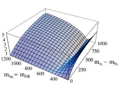
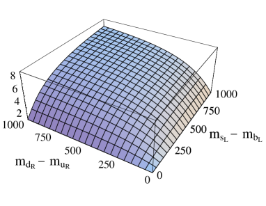
Figure 6: Left: QCD penguin coefficient $|c_{2}^{\rm QCD}|$ in units of $10^{-4}|\sin 2\theta_{L}|$ versus the common mass $m_{\tilde{u}_{R}}=m_{\tilde{d}_{R}}$ (left axis) and the mass splitting $m_{\tilde{s}_{L}}-m_{\tilde{b}_{L}}$ (right axis), for $m_{\tilde{b}_{L}}=m_{\tilde{g}}=250$ GeV. Right: Electroweak penguin coefficient $|c_{2}^{\rm EW}|$ in units of $10^{-4}|\sin 2\theta_{L}|$ versus the mass splittings $m_{\tilde{d}_{R}}-m_{\tilde{u}_{R}}$ (left axis) and $m_{\tilde{s}_{L}}-m_{\tilde{b}_{L}}$ (right axis), for $m_{\tilde{u}_{R}}=m_{\tilde{b}_{L}}=m_{\tilde{g}}=250$ GeV. All masses are given in GeV.

We are now ready to present our numerical results. We begin with the SUSY contributions to the penguin coefficients at the SUSY matching scale, which for simplicity we take to be $m_{W}$, thus ignoring the slow running of $\alpha_{s}$ and superpartner masses above the weak scale. We find that the QCD coefficients obey the approximate scaling relation $c_{2}^{\rm QCD}\sim c_{4}^{\rm QCD}\sim-3c_{1}^{\rm QCD}\sim-3c_{3}^{\rm QCD}$ (provided we use the same masses for left- and right-handed squarks), which according to (74) is exact for the contributions of the penguin diagrams but only approximate for the box diagrams. The coefficients $\widetilde{c}_{i}^{\rm QCD}$ are the same as the $c_{i}^{\rm QCD}$ if all labels $L\leftrightarrow R$ are interchanged. In the left-hand plot in Figure 6 we show the largest coefficient, $c_{2}^{\rm QCD}$, for a common mass $m_{\tilde{b}_{L}}=m_{\tilde{g}}=250$ GeV as a function of the mass splitting between the left-handed strange and bottom squarks and of the common mass $m_{\tilde{u}_{R}}=m_{\tilde{d}_{R}}$. Note that only the box contributions in (5.1) depend on the latter two masses, but not the penguin contributions in (74). We find that these two contributions interfere destructively. For small up- and down-squark masses the box contributions are dominant, whereas for large masses the boxes decouple and the penguin contributions dominate. For intermediate masses there is a region with large destructive interference, where $c_{2}^{\rm QCD}$ vanishes or takes small values. Note that typical values of the coefficients $c_{i}^{\rm QCD}$ are of order few times $10^{-4}$ (provided the gluino is as light as 250 GeV and there is sufficient mass splitting between the strange and bottom squarks), which is an order of magnitude less than the typical size of QCD penguin coefficients in the SM [10]. If the gluino mass is increased and all mass ratios remain the same, then the SUSY contributions to the Wilson coefficients decrease, scaling like $(250\,\mbox{GeV}/m_{\tilde{g}})^{2}$.

We next turn to the coefficients of the electroweak penguin operators, which only receive contributions from the gluino box diagrams. As mentioned above, because of SU(2)_L symmetry only $c_{1}^{\rm EW}$, $c_{2}^{\rm EW}$, $\widetilde{c}_{3}^{\rm EW}$ and $\widetilde{c}_{4}^{\rm EW}$ are important, and we find that for equal strange–bottom mixing and mass splitting in the left-handed and right-handed squark sectors they roughly scale according to $c_{2}^{\rm EW}\sim\widetilde{c}_{4}^{\rm EW}\sim-3c_{1}^{\rm EW}\sim-3\widetilde{c}_{3}^{\rm EW}$. In the right-hand plot in Figure 6 we show the largest coefficient, $c_{2}^{\rm EW}$, as a function of the mass splittings between the left-handed strange and bottom squarks and between the right-handed up and down squarks. Provided both splittings are significant, the typical values of the electroweak penguin coefficients are of order few times $10^{-4}$, which is comparable with the value of the coefficient $c_{3}^{\rm EW}$ in the SM, given in (2). Therefore, in certain regions of SUSY parameter space there can be important isospin-violating contributions to the parameters $a$ and $b$ entering the $B^{\pm}\to\pi K$ decay amplitudes. An important point to notice is that SUSY contributions to the electroweak penguin coefficients are typically of same order as, or can be larger than, the contributions to the QCD penguin coefficients, if there is sufficient mass splitting between the right-handed up and down squarks.

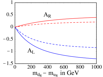
Figure 7: Quantities $A_{R}$ (two upper curves) and $A_{L}$ (two lower curves) versus the mass splitting $m_{\tilde{d}_{R}}-m_{\tilde{u}_{R}}$, for $m_{\tilde{u}_{R}}=m_{\tilde{b}_{L,R}}=m_{\tilde{g}}=250$ GeV. The solid curves refer to $m_{\tilde{s}_{L,R}}=1000$ GeV, the dashed ones to $m_{\tilde{s}_{L,R}}=500$ GeV.

The SUSY contributions to the parameters $a$ and $b$ can be decomposed as

$$(a_{\rm NP}+ib)_{\rm SUSY}$$ (80)

$$=A_{L}\sin 2\theta_{L}\,e^{i\delta_{L}}+A_{R}\sin 2\theta_{R}\,e^{i\delta_{R}}\,,$$

where $A_{L}$ receives contributions from the electroweak penguin coefficients $c_{1}^{\rm EW}$ and $c_{2}^{\rm EW}$, and $A_{R}$ receives contributions from $\widetilde{c}_{3}^{\rm EW}$ and $\widetilde{c}_{4}^{\rm EW}$. As previously mentioned, to obtain large values of these parameters requires a significant mass splitting between the right-handed up and down squarks, as well as a substantial splitting between the left- or right-handed strange and bottom squarks. Exchanging strange and bottom or up and down squarks leaves the results invariant up to a sign. In Figure 7 we show the values of $A_{L}$ and $A_{R}$ versus $m_{\tilde{d}_{R}}-m_{\tilde{u}_{R}}$ for two choices of the strange–bottom splitting, such that $m_{\tilde{s}_{L,R}}/m_{\tilde{b}_{L,R}}=2$ or 4. We note that for large mass splittings the magnitude of $A_{L}$ can be up to twice the SM parameter $\delta_{\rm EW}\approx 0.64$, whereas for more moderate splittings $|A_{L}|\sim\delta_{\rm EW}$ can be obtained. The magnitude of the parameter $A_{R}$ is typically smaller by a factor of 3. According to Figure 5, SUSY contributions of this size could lead to shifts of up to $\pm 50^{\circ}$ in the extracted value of $\gamma_{\pi K}$. Even in the more realistic case where only right-handed strange–bottom squark mixing is large, shifts of up to $\pm 25^{\circ}$ are possible.

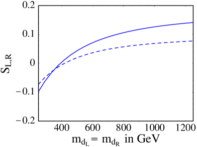
Figure 8: Quantities $S_{L,R}$ versus the common mass $m_{\tilde{d}_{L}}=m_{\tilde{d}_{R}}$, for $m_{\tilde{b}_{L,R}}=m_{\tilde{g}}=250$ GeV. The solid curve refers to $m_{\tilde{s}_{L,R}}=1000$ GeV, the dashed one to $m_{\tilde{s}_{L,R}}=500$ GeV.

Let us now briefly discuss SUSY contributions to the parameter $\rho$ describing CP-violating but isospin-conserving New Physics effects in $B^{\pm}\to\pi K$ decays. From (20) it follows that QCD penguin coefficients of order few times $10^{-4}$ can only lead to rather small values $|\rho|\ \hbox to0.0pt{\raise 3.0pt\hbox{$<$}\hss}{\lower 3.0pt\hbox{$\sim$}}\ 0.1$. In analogy with (80), we define

$$(\sin\varphi)_{\rm SUSY}$$ (81)

$$=S_{L}\sin 2\theta_{L}\sin\delta_{L}-S_{R}\sin 2\theta_{R}\sin\delta_{R}\,,$$

where $S_{L}$ ($S_{R}$) depends on the mass splitting between the left-handed (right-handed) strange and bottom squarks, and both quantities depend on the masses of the left- and right-handed down squarks. In Figure 8 we show the values of these quantities versus the common down-squark mass for two choices of the strange–bottom splitting. We see that, indeed, typical values of $S_{L}$ and $S_{R}$ are of order 0.1 or less. The corresponding contributions to $\rho$ are of the same order for maximal weak phases and large strange–bottom mixing. According to Figure 5, SUSY contributions of this size can only lead to insignificant shifts in the extracted value of $\gamma_{\pi K}$.

Thus far we have only considered contributions to $\rho$ due to the four-quark penguin operators. The largest possible contributions in fact arise if the coefficient $C_{8g}$ of the chromomagnetic dipole operator, or the coefficient $\widetilde{C}_{8g}$ of the corresponding dipole operator with opposite chirality, have very large magnitudes compared with their values in the SM, implying enhanced $\bar{b}\to\bar{s}g$ transitions. This scenario has been discussed in the context of the low semileptonic branching ratio and charm yield in $B$ decays [34, 35, 57] and the large $B\to X_{s}\,\eta^{\prime}$ branching ratio [58, 59, 60]. In SUSY models it is most easily realized via gluino–squark loops containing left–right strange–bottom squark mass insertions [33, 35, 36, 46]. Constraints on these graphs from $B\to X_{s}\,\gamma$ decays allow for $\mbox{B}(B\to X_{sg})\ \hbox to0.0pt{\raise 3.0pt\hbox{$<$}\hss}{\lower 3.0pt\hbox{$\sim$}}\ 10\%$, which corresponds to $(|C_{8g}|^{2}+|\widetilde{C}_{8g}|^{2})^{1/2}\approx 1$ (at the scale $m_{b}$), together with possibly large CP-violating phases in these coefficients [61]. From (20) it follows that large values $\rho=O(1)$ can be obtained in such a scenario. According to Figure 5, in this extreme case large shifts in the value of $\gamma_{\pi K}$ caused by isospin-conserving New Physics are not excluded.

At present, there are no significant phenomenological constraints on the angles $\theta_{L}$ and $\theta_{R}$ parameterizing the mixing between the strange and bottom squarks. In particular, the measured $B\to X_{s}\,\gamma$ branching ratio does not impose a useful constrain on these parameters. However, an important constraint would emerge if in the future $B_{s}$–$\bar{B}_{s}$ mixing were found to be consistent with, or not much larger than, its predicted value in the SM. For simplicity, we assume that only one of the two mixing angles is large. In the case of left-handed squark mixing, for instance, the relevant gluino box contribution to the $B_{s}$–$\bar{B}_{s}$ mass difference $\Delta m_{s}$, normalized to the SM contribution, is given by [46]

$$\left|\frac{\Delta m_{s}^{LL}}{\Delta m_{s}^{\rm SM}}\right| = \frac{\sin^{2}\!2\theta_{L}}{|\lambda_{t}|^{2}}\,\frac{\alpha_{s}^{2}}{\alpha_{W}^{2}}\,\frac{m_{W}^{2}}{m_{\tilde{g}}^{2}}\,\frac{1}{C(x_{t})}$$ (82)

$$\times \Bigg{|}\frac{11}{18}\Big{[}G(x_{\tilde{b}_{L}\tilde{g}},x_{\tilde{b}_{L}\tilde{g}})+G(x_{\tilde{s}_{L}\tilde{g}},x_{\tilde{s}_{L}\tilde{g}})-2G(x_{\tilde{b}_{L}\tilde{g}},x_{\tilde{s}_{L}\tilde{g}})\Big{]}$$

$$\mbox{}-\frac{2}{9}\Big{[}F(x_{\tilde{b}_{L}\tilde{g}},x_{\tilde{b}_{L}\tilde{g}})+F(x_{\tilde{s}_{L}\tilde{g}},x_{\tilde{s}_{L}\tilde{g}})-2F(x_{\tilde{b}_{L}\tilde{g}},x_{\tilde{s}_{L}\tilde{g}})\Big{]}\Bigg{|}\,,$$

where $x_{t}=m_{t}^{2}/m_{W}^{2}$, and

$$C(x)=\frac{x^{4}-12x^{3}+15x^{2}-2x+6x^{3}\ln x}{4(x-1)^{3}}\,.$$ (83)

For right-handed squark mixing the ratio $|\Delta m_{s}^{RR}/\Delta m_{s}^{\rm SM}|$ would be obtained from the above result via the substitution $L\to R$.

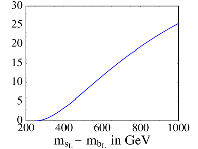
Figure 9: Ratio $|\Delta m_{s}^{LL}/\Delta m_{s}^{\rm SM}|$ in units of $\sin^{2}\!2\theta_{L}$ versus the mass splitting $m_{\tilde{s}_{L}}-m_{\tilde{b}_{L}}$ in GeV, for $m_{\tilde{b}_{L}}=m_{\tilde{g}}=250$ GeV.

In Figure 9 the ratio of the SUSY contribution to $\Delta m_{s}$ to the SM result is shown as a function of the mass splitting between strange and bottom squarks. The same plot with obvious substitutions $L\to R$ applies to the case of mixing between the right-handed squarks. We observe that $\Delta m_{s}$ would greatly exceed the SM value in regions of parameter space associated with large SUSY contributions to the penguin coefficients. To gauge the potential impact of a $\Delta m_{s}$ measurement near the predicted SM value we impose as an example the hypothetical constraint that $|\Delta m_{s}^{LL}/\Delta m_{s}^{\rm SM}|\leq 2$. According to Figure 9, it then follows that, e.g., $|\sin 2\theta_{L}|<0.52$ for $m_{\tilde{s}_{L}}=2m_{\tilde{b}_{L}}=500$ GeV, and $|\sin 2\theta_{L}|<0.28$ for $m_{\tilde{s}_{L}}=4m_{\tilde{b}_{L}}=1000$ GeV. Hence, if such a constraint would have to be imposed in the future, the allowed magnitude of the SUSY contributions to the penguin coefficients would be reduced by a significant amount. (Note, however, that the coefficients of the chromomagnetic dipole operators are very weakly constrained by $B_{s}$–$\bar{B}_{s}$ mixing.)

Finally, we comment on implications of naturalness for the large right-handed up–down squark mass splitting necessary to obtain sizable SUSY contributions to the electroweak penguin coefficients. Following [62] we note that in models in which SUSY is broken at high energies, e.g., supergravity, there is a naturalness constraint on the squark and slepton mass spectrum coming from the hypercharge $D$-term. In these models the $Z$-boson mass is given by

$$\frac{m_{Z}^{2}}{2}=\frac{m_{1}^{2}-m_{2}^{2}\tan^{2}\!\beta}{\tan^{2}\!\beta-1}\,,$$ (84)

where $m_{1}^{2}$, $m_{2}^{2}$ and $\tan\beta$ are the usual parameters of the Higgs potential in the minimal SUSY extension of the SM [63]. The renormalization-group equations give

$$m_{2}^{2} = -\frac{1-Z_{1}}{22}\,\mbox{Tr}\,\Big{(}m_{\tilde{Q}_{L}}^{2}+m_{\tilde{d}_{R}}^{2}-2m_{\tilde{u}_{R}}^{2}-m_{\tilde{L}_{L}}^{2}+m_{\tilde{e}_{R}}^{2}\Big{)}+\hat{m}_{2}^{2}\,,$$

$$Z_{1} = \left(1+\frac{33}{20\pi}\,\alpha_{\rm GUT}\ln\frac{M_{\rm GUT}^{2}}{m_{\rm SUSY}^{2}}\right)^{-1}\approx 0.4\,,$$ (85)

where $m_{A}^{2}$ ($A=\tilde{Q}_{L},\tilde{u}_{R},\tilde{d}_{R},\tilde{L}_{L},\tilde{e}_{R}$) are the values of the squark and slepton masses at the GUT scale, $\hat{m}_{2}^{2}$ contains the dependence on the other soft SUSY breaking masses, and the trace is taken over generation space. It is clear from (5.1) that a large mass splitting between the first generation right-handed up and down squarks poses a potential naturalness problem. However, the hypercharge $D$-term can vanish in GUT theories in which hypercharge is embedded in the GUT group. For example, in SU(5) one has the relations

$$m_{\tilde{Q}_{L}}^{2}=m_{\tilde{u}_{R}}^{2}=m^{2}_{\tilde{e}_{R}}\equiv m_{10}^{2}\,,\qquad m_{\tilde{d}_{R}}^{2}=m_{\tilde{L}_{L}}^{2}=m_{\bar{5}}^{2}\,,$$ (86)

so that it is possible to have large up–down squark-mass splitting without encountering difficulties with naturalness.

To summarize, we have seen that SUSY contributions to the Wilson coefficients of the penguin operators in the effective Hamiltonian for $\bar{b}\to\bar{s}q\bar{q}$ transitions, and in particular of the isospin-violating electroweak penguin operators, can be substantial if the gluino and certain squarks have masses near the weak scale, and other squarks have masses near a TeV. Large left-handed or right-handed strange–bottom squark mixing is also required. The latter option is naturally realized in certain SUSY theories of flavor.

5.2 Two-Higgs–doublet models

In extensions of the SM containing charged Higgs bosons [63] there are new photon and Z penguin diagrams contributing to the Wilson coefficients of the penguin operators. Here we consider a general class of two-Higgs–doublet models (2HDMs) discussed in [64], which contains the conventional type-1 and type-2 2HDMs as special cases. We find that, if terms of order $m_{b}/m_{t}$ are neglected, the new penguin contributions only involve the $Ht_{R}b_{L}$ coupling. Following [64] we write the corresponding term in the Lagrangian as

$${\cal L}_{Ht_{R}b_{L}}=-\xi_{t}\,m_{t}\,\bar{b}_{Lj}V_{ji}^{\dagger}\,t_{Ri}\,H^{-}+\mbox{h.c.},$$ (87)

where $V_{ij}$ is the CKM matrix. In principle, the parameter $\xi_{t}$ may contain a CP-violating phase. However, the penguin contributions only depend on $|\xi_{t}|^{2}$, and thus any weak phase would cancel out. This conclusion holds true even in a wider class of multi-Higgs models [65]. It is therefore sufficient to focus on the conventional type-1 or type-2 two-Higgs–doublet models, for which $|\xi_{t}|^{2}=\cot^{2}\!\beta$.

It follows from the above discussion that in 2HDMs there are no New Physics contributions to the CP-violating parameters $\rho$ and $b$ entering the parametrization of the $B^{\pm}\to\pi K$ decay amplitudes in (3.1). Therefore, it is sufficient for our purposes to focus on the electroweak penguin coefficients, which induce a new contribution to the parameter $a$. Including both the photon and Z penguin diagrams, one obtains at the weak scale [66, 67]

$$c_{1}^{\rm EW} = \frac{\alpha\lambda_{t}}{8\pi}\cot^{2}\!\beta\left[x_{t}\,f(x_{tH})+\frac{1}{9}\,g(x_{tH})\right]\,,$$

$$c_{3}^{\rm EW} = \frac{\alpha\lambda_{t}}{8\pi}\cot^{2}\!\beta\left[-x_{t}\cot^{2}\!\theta_{W}\,f(x_{tH})+\frac{1}{9}\,g(x_{tH})\right]\,,$$ (88)

where $x_{tH}=(m_{t}/m_{H^{+}})^{2}$, and

$$f(x) = \frac{x}{1-x}+\frac{x\ln x}{(1-x)^{2}}\,,$$

$$g(x) = \frac{38x-79x^{2}+47x^{3}}{6(1-x)^{3}}+\frac{4x-6x^{2}+3x^{4}}{(1-x)^{4}}\ln x\,.$$ (89)

In this model there is a simple result for the New Physics contribution to the parameter $a$, normalized to the SM contribution. We find

$$\frac{a_{\rm NP}}{\delta_{\rm EW}}=-\cot^{2}\!\beta\,\frac{f(x_{tH})}{1+\frac{3\ln x_{t}}{x_{t}-1}}\left\{1-0.74\sin^{2}\!\theta_{W}\left[1+\frac{g(x_{tH})}{9x_{t}\,f(x_{tH})}\right]\right\}\,,$$ (90)

where the first term in parenthesis is free of hadronic uncertainties, and the second term is numerically small.

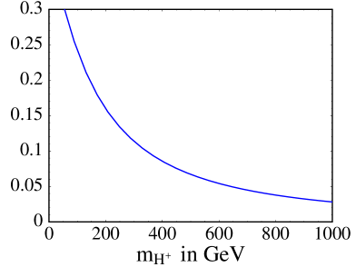
Figure 10: Ratio $a_{\rm NP}/\delta_{\rm EW}$ in units of $\cot^{2}\!\beta$ in a general 2HDM, as a function of the charged-Higgs mass.

In Figure 10, we show the ratio $a_{\rm NP}/\delta_{\rm EW}$ in units of $\cot^{2}\!\beta$ as a function of the Higgs mass. Even for $\cot\beta=1$ a significant contribution to the parameter $a$ requires a small Higgs mass. This possibility is not excluded by direct searches, however in the context of specific models the constraint from the $B\to X_{s}\,\gamma$ branching ratio often favors a larger mass and $\cot^{2}\!\beta<1$ [68, 69]. Therefore, it appears unlikely that a large new contribution to $a$ can be obtained in 2HDMs.

5.3 Models with anomalous gauge-boson couplings

The SU(2)${}_{L}\times\mbox{U(1)}_{Y}$ gauge symmetry of the SM fully determines the form of the dimension-4 operators that describe the vector-boson self-couplings. New Physics may induce anomalous couplings of the electroweak gauge bosons, which at low energies give rise to higher-dimensional operators, whose effects are suppressed by inverse powers of the New Physics scale $\Lambda$. The effects of anomalous gauge-boson couplings on rare $B$ decays have been investigated in [40, 70], and their impact on the determination of $\gamma$ from $B^{\pm}\to\pi K$ decays has been discussed in [19]. A general parametrization of the anomalous gauge-boson couplings can be found in [71]. In low-energy processes, the four new parameters that enter are $\Delta\kappa^{\gamma}$, $\Delta g_{1}^{Z}$, $\lambda^{\gamma}$ and $g_{5}^{Z}$. The first two represent corrections to couplings already present in the SM, whereas the latter two refer to new vertices. Note that these four parameters are real and thus can only contribute to the quantity $a$, but not to $\rho$ and $b$. As in the previous section, we therefore focus only on the coefficients of the electroweak penguin operators. They are [72]

$$c_{1}^{\rm EW} = \frac{\alpha\lambda_{t}}{8\pi}\,x_{t}\Big{[}\cos^{2}\!\theta_{W}\,f_{A}(x_{t})+h_{A}(x_{t})\Big{]}\,,$$

$$c_{3}^{\rm EW} = \frac{\alpha\lambda_{t}}{8\pi}\,x_{t}\left[-\cot^{2}\!\theta_{W}\cos^{2}\!\theta_{W}\,f_{A}(x_{t})+h_{A}(x_{t})\right]\,,$$ (91)

with

$$f_{A}(x) = -3\Delta g_{1}^{Z}\ln\frac{\Lambda^{2}}{m_{W}^{2}}+\frac{6g_{5}^{Z}}{1-x}\left(1+\frac{x\ln x}{1-x}\right)\,,$$

$$h_{A}(x) = \frac{\Delta\kappa^{\gamma}}{2}\ln\frac{\Lambda^{2}}{m_{W}^{2}}+\lambda^{\gamma}\left[\frac{1-3x}{(1-x)^{2}}-\frac{2x^{2}\ln x}{(1-x)^{3}}\right]\,,$$ (92)

where the New Physics scale $\Lambda$ acts as an ultraviolet cutoff.

As in the case of the 2HDMs, there is a very simple result for the New Physics contribution to the parameter $a$, normalized to the SM contribution. We find

$$\frac{a_{\rm NP}}{\delta_{\rm EW}}=-\cos^{2}\!\theta_{W}\,\frac{f_{A}(x_{t})}{1+\frac{3\ln x_{t}}{x_{t}-1}}\left\{1-0.74\sin^{2}\!\theta_{W}\left[1+\frac{h_{A}(x_{t})}{\cos^{2}\!\theta_{W}\,f_{A}(x_{t})}\right]\right\}\,,$$ (93)

where as before the first term in parenthesis is free of hadronic uncertainties. For instance, taking $\Lambda=1$ TeV gives

$$\frac{a_{\rm NP}}{\delta_{\rm EW}}\approx 4.20\Delta g_{1}^{Z}-0.45g_{5}^{Z}+0.19\Delta\kappa^{\gamma}+0.03\lambda^{\gamma}\,.$$ (94)

From naive dimensional analysis, one expects that $\Delta g_{1}^{Z},\Delta\kappa^{\gamma}\sim(g_{W}v/\Lambda)^{2}\sim 10^{-2}$ (with $v\approx 246$ GeV the Higgs vacuum expectation value), whereas $g_{5}^{Z}$ and $\lambda^{\gamma}$ are expected to be further suppressed [70, 73]. Potentially the most important contribution in (94) is due to $\Delta g_{1}^{Z}$, which is bounded by experiment to lie in the range $-0.113<\Delta g_{1}^{Z}<0.126$ [74]. Even when this bound is saturated, $a_{\rm NP}/\delta_{\rm EW}$ cannot exceed 0.5 in magnitude. However, from naive dimensional analysis $a_{\rm NP}$ is naturally an order of magnitude smaller.

6 Conclusions

We have explored how New Physics could affect purely hadronic FCNC transitions of the type $\bar{b}\to\bar{s}q\bar{q}$ focusing, in particular, on isospin violation. Unlike in the Standard Model, where isospin-violating effects in these processes are strongly suppressed by electroweak gauge couplings or small CKM matrix elements, in many New Physics scenarios these effects are not parametrically suppressed relative to isospin-conserving FCNC processes. In the language of effective weak Hamiltonians, this implies that the Wilson coefficients of QCD and electroweak penguin operators are of a similar magnitude. For a large class of New Physics models, we find that the coefficients of the electroweak penguin operators are, in fact, due to “trojan” penguins, which are neither related to penguin diagrams nor of electroweak origin.

We have calculated the Wilson coefficients of the penguin operators in the effective weak Hamiltonian in several New Physics models, extending the usual operator basis where appropriate. We have also included penguin operators mediating the decay $\bar{b}\to\bar{d}s\bar{d}$, which is highly suppressed in the Standard Model. Specifically, we have considered: (a) models with tree-level FCNC couplings of the $Z$ boson, extended gauge models with an extra $Z^{\prime}$ boson, SUSY models with broken R-parity; (b) SUSY models with R-parity conservation; (c) two-Higgs–doublet models, and models with anomalous gauge-boson couplings. In case (a), the resulting electroweak penguin coefficients can be much larger than in the Standard Model because they are due to tree-level processes. In case (b), these contributions can compete with the Standard Model coefficients because they arise from strong-interaction box diagrams, which scale relative to the Standard Model like $(\alpha_{s}/\alpha)(m_{W}^{2}/m_{\rm SUSY}^{2})$. In models (c), on the other hand, isospin-violating New Physics effects are not parametrically enhanced and are generally smaller than in the Standard Model.

We have focused on the rare hadronic decays $B^{\pm}\to\pi K$, which are particularly sensitive to isospin-violating effects. These decays are especially useful for probing New Physics contributions, since in the Standard Model the theoretical description of such effects is very clean. We have found that the ratio $R_{*}$ of the CP-averaged branching ratios defined in (23) and the value of the weak phase $\gamma_{\pi K}$ extracted from $B^{\pm}\to\pi K$ decays are the most useful observables for probing isospin-violating New Physics contributions. Using a fully general parametrization of the decay amplitudes, we have derived model-independent bounds on $R_{*}$ in the presence of New Physics, and have investigated by how much $\gamma_{\pi K}$ could differ from the true value of the CKM angle $\gamma$. We have seen that, depending on the measured value of $R_{*}$, it may be possible to unambiguously distinguish between isospin-violating and isospin-conserving New Physics contributions. Irrespective of the value of $R_{*}$, we find that large shifts in $\gamma$ can be caused by even moderate isospin-violating contributions to the decay amplitudes of order 10%. In contrast, significant shifts due to isospin-conserving New Physics effects would require a new $O(1)$ CP-violating contribution to the amplitudes.

Model	$|a_{\rm NP}+ib|$	$|\gamma_{\pi K}-\gamma|$	$|\rho|$	$|\gamma_{\pi K}-\gamma|$
FCNC $Z$ exchange	2.0	$180^{\circ}$	0.05	$3^{\circ}$
extra $Z^{\prime}$ boson	14∗	$180^{\circ}$	–	$180^{\circ}$
SUSY without R-parity	14∗	$180^{\circ}$	–	$180^{\circ}$
SUSY with R-parity	0.4	$25^{\circ}$	0.12	$7^{\circ}$
	1.3	$180^{\circ}$	0.12	$7^{\circ}$
2HDM	0.15	$10^{\circ}$	0	$0^{\circ}$
anom. gauge-boson coupl.	0.3	$20^{\circ}$	0	$0^{\circ}$

Table 1: Maximal contributions to the relevant phenomenological parameters, as defined in the text. Entries for $\rho$ containing a “–” are unconstrained. Entries marked with a “^∗” are upper bounds obtained using the current values of $\bar{\varepsilon}_{3/2}$ and $R_{*}$. For the case of SUSY with R-parity the first (second) row corresponds to maximal right-handed (left-handed) strange–bottom squark mixing. For the 2HDM we take $m_{H^{+}}>100$ GeV and $\tan\beta>1$.

For each New Physics model we have explored which regions of parameter space can be probed by the $B^{\pm}\to\pi K$ observables, and how big a departure from the Standard Model predictions one can expect under realistic circumstances. In Table 1, we summarize our estimates of the maximal isospin-violating and isospin-conserving contributions to the decay amplitudes, as parameterized by $|a_{\rm NP}+ib|$ and $|\rho|$, respectively. For comparison, we recall that in the Standard Model $a\approx 0.64$ and $b\approx\rho\approx 0$. We also list the corresponding maximal values of the difference $|\gamma_{\pi K}-\gamma|$. As noted above, in models with tree-level FCNC couplings New Physics effects can be dramatic, whereas in SUSY models with R-parity conservation isospin-violating loop effects can be competitive with the Standard Model. In the case of SUSY models with R-parity violation, we have derived interesting bounds on combinations of the trilinear couplings $\lambda_{ijk}^{\prime}$ and $\lambda_{ijk}^{\prime\prime}$, which are given in (4.3) and (4.3).

It is worth pointing out that isospin- or, more generally, SU(3) flavor-violating New Physics effects in hadronic weak decays could also be important in other processes. For instance, they have been shown to yield a potentially large contribution to the quantity $\epsilon^{\prime}/\epsilon$ in $K\to\pi\pi$ decays [15]. Moreover, there are other $B$ and $B_{s}$ decay channels that could be sensitive to flavor-violating New Physics contributions. We look forward to returning to this subject in an extra dimension.