LA-UR-99-4856

TMUP-HEL-9911

YCTP-P23-99

hep-ph/9909296

A Two-dimensional Model with Chiral Condensates and Cooper Pairs having QCD-like Phase Structure

Alan Chodos
  Department of Physics, Yale University, New Haven, CT 06520-8120

Fred Cooper

Los Alamos National Laboratory, Los Alamos, NM 87545

Wenjin Mao

Department of Physics, Boston College, Chestnut Hill, MA 02467

Hisakazu Minakata

Department of Physics, Tokyo Metropolitan University
Minami-Osawa, Hachioji, Tokyo 192-0397, Japan and
Research Center for Cosmic Neutrinos, Institute for Cosmic Ray Research
University of Tokyo, Tanashi, Tokyo 188-8502, Japan

Anupam Singh

Los Alamos National Laboratory, Los Alamos, NM 87545

Abstract

We generalize our previous model[9] to an O(N) symmetric two-dimensional model which possesses chiral symmetry breaking ($\langle\bar{\psi}\psi\rangle$ condensate) and superconducting (Cooper pair $\langle\psi\psi\rangle$ condensates) phases at large-N. At zero temperature and density, the model can be solved analytically in the large-N limit. We perform the renormalization explicitly and obtain a closed form expression of the effective potential. There exists a renormalization group invariant parameter $\delta$ that determines which of the $\langle\bar{\psi}\psi\rangle$ ($\delta>0$) or $\langle\psi\psi\rangle$ ($\delta<0$) condensates exist in the vacuum. At finite temperatures and densities, we map out the phase structure of the model by a detailed numerical analysis of the renormalized effective potential. For $\delta$ positive and sufficiently large, the phase diagram in the $\mu$-$T$ (chemical potential-temperature) plane exactly mimics the features expected for QCD with two light flavors of quarks. At low temperatures there exists low-$\mu$ chiral symmetry breaking and high-$\mu$ Cooper pair condensate regions which are separated by a first-order phase transition. At high $\mu$, when the temperature is raised, the system undergoes a second-order phase transition from the superconducting phase to an unbroken phase in which both condensates vanish. For a range of values of $\delta$ the theory possesses a tricritical point ($\mu_{tc}$ and $T_{tc}$); for $\mu>\mu_{tc}$ ($\mu<\mu_{tc}$) the phase transition from the low temperature chiral symmetry breaking phase to unbroken phase is first-order (second-order). For the range of $\delta$ in which the system mimics QCD, we expect the model to be useful for the investigation of dynamical aspects of nonequilibrium phase transitions, and to provide information relevant to the study of relativistic heavy ion collisions and the dense interiors of neutron stars.

PACS numbers:

I Introduction

The phase structure of $QCD$ at non-zero temperature and baryon density is important for the physics of neutron stars and heavy ion collisions.

An approximate phase structure for QCD with two massless quarks has been mapped out in various mean field and perturbative approximations and a rich structure has emerged. For a recent review, see [1]. In addition to the well known chiral symmetry broken and restored phases recent investigations have revealed the possibility of a color superconducting phase at low temperatures and relatively high densities [2] [3] [4]. In the chiral condensation regime at zero chemical potential, the phase transition to the unbroken mode is second order as we raise the temperature [5]. As we increase the chemical potential at fixed low temperature there is a first order transition to a superconducting phase. There is also a regime where as we increase the temperature the phase transition from the chirally broken phase to the unbroken phase is first order, so that somewhere along the line separating these phases there is a tricritical point [6]. These results are summarized in [1].

One of the more interesting questions is what happens in a dynamical situation such as a heavy ion collision, in which the system traverses the various phase transitions as it expands and cools. One would like to study the correlation functions to see whether there is qualitatively different behavior in crossing the first order or second order transition regions as a function of the proper evolution time and whether this difference would lead to some interesting experimental signatures at RHIC.

In order to get a better handle on this latter question, we propose a simple 1+1 dimensional model which contains several of the features of two flavor massless QCD in mean field approximation (similar phase structure and asymptotic freedom) which would lend itself to dynamical computational simulations pertinent to the (one dimensional) expansion of a Lorentz contracted disc of quark matter. Thus we hope to explore the behavior of a system of “quarks” evolving through first and second order phase transitions to either a final state with chiral condensates or to a superconducting final state. This calculation would be similar in spirit to those that were done in exploring the chiral phase transition in the linear sigma model [7].

In this paper we restrict ourselves to mapping out the phase structure of our model at finite temperature and chemical potential in a large-$N$ approximation, for use in obtaining initial conditions for our future dynamical calculations. Our simple model combines the Gross-Neveu model [8] with a model for Cooper pairs that we introduced recently [9]. It turns out to have many of the features of QCD that we ultimately want to capture in more realistic calculations. Namely, the theory in the Gross-Neveu sector has the same second-order, first-order, tricritical point behavior for the chiral condensate $<\bar{q}q>$ as a function of temperature [10] and chemical potential [10] [11] as QCD with two massless flavors. Adding the second interaction also adds a new phase where there is superconductivity at some finite chemical potential as also expected in QCD with two massless flavors. The model has a well defined $1/N$ expansion and is asymptotically free so that it does not suffer from the cutoff dependences of $3+1$ dimensional effective field theories considered by others [2] [3].

Thus we will be investigating a 1+1 dimensional model governed by two independent couplings:  the original Gross-Neveu term [8] that promotes the condensation of $\langle\bar{q}q\rangle$, and the term considered in our earlier paper [9]that produces a $\langle qq\rangle$ condensate. We first determine the unrenormalized effective potential at leading order in a large-N expansion, by introducing collective coordinates for the $\bar{q}q$, and $qq$ operators, and integrating out the fermions in the usual fashion by using the Hubbard-Stratonovich trick [12].

At zero temperature and chemical potential we derive a closed-form analytic expression for the renormalized effective potential. We find that there is one dimensionless parameter $\delta$, independent of the renormalization scale, whose value determines which of the condensates is present. This situation might be described as “partial dimensional transmutation”: the unrenormalized theory has two bare couplings whereas the renormalized one has a renormalization scale, which is arbitrary (but which can be related to the physical fermion or Cooper pair gap mass) , and a dimensionless parameter $\delta$ independent of this scale, that controls the physics. We find that the gap equations have three types of solution:  two in which one or the other of the condensates vanish, and a third, mixed case, in which both condensates are non-vanishing. It turns out, however, that the true minimum of the effective potential is at a point where one of the condensates vanishes except at the particular point $\delta=0$ (to be discussed further below)where one is at a first order phase transition so that phase coexistence can occur. Depending on the sign of $\delta$ we therefore have very different behavior at zero temperature and chemical potential– namely either chiral condensates or Cooper-pairs being present.

The phase structure of the limiting theories which have only one coupling constant is easy to determine analytically, and we include for completeness a discussion of these two particular cases which benchmark our numerical study of the general case. Performing the integration in our expression for the renormalized effective potential numerically, we then map out the phase diagram for the more general two coupling constant case as a function of $\delta$. We find a regime of (positive) $\delta$ which remarkably mimics the phase structure of two flavor QCD described above. It has a tricritical point as well as a first order phase transition as a function of chemical potential from the chirally broken phase into the superconducting phase. We determine the tricritical point and the critical temperature at which the superconducting phase transition occurs as a function of $\delta$. As we decrease the magnitude of $\delta$, first the regime of first order phase transition from the chiral phase disappears, and then at the special point $\delta=0$ the possibility of a chiral symmetry broken phase totally disappears so that when $\delta<0$ one only has the possibility for a superconducting broken symmetry mode at low temperatures.

II General Considerations

We consider the most general Lagrangian with quartic fermion couplings, possessing $O(N)$ flavor symmetry and discrete chiral symmetry.

$${\cal L} = \bar{\psi}^{(i)}i\bigtriangledown\!\!\!\!\!\!/\psi^{(i)}+{1\over 2}g^{2}[\bar{\psi}^{(i)}\psi^{(i)}][\bar{\psi}^{(j)}\psi^{(j)}]$$ (1)

$$+ 2G^{2}(\bar{\psi}^{(i)}\gamma_{5}\psi^{(j)})(\bar{\psi}^{(i)}\gamma_{5}\psi^{(j)})-\mu\psi^{\dagger(i)}\psi^{(i)}.$$ (2)

The flavor indices, summed on from $1$ to $N$, have been explicitly indicated. The first quartic term is the usual Gross-Neveu interaction, whereas the second such term, which differs in the arrangement of its flavor indices, induces the pairing force to leading order in ${1\over N}$. This term is possible because we demand only $O(N)$ symmetry as opposed to the $SU(N)$ symmetry of the original Gross-Neveu model. In the final term, $\mu$ is the chemical potential.

Strictly speaking, a $\langle\psi\psi\rangle$ condensate cannot form, because it breaks the $U(1)$ of Fermion number and hence violates Coleman’s theorem [13]. Similarly, $\langle\bar{\psi}\psi\rangle$ as well as $\langle\psi\psi\rangle$ condensates cannot exist at finite temperature in one spatial dimension because of the Mermin-Wagner theorem [13]. Nevertheless, it is meaningful to study the formation of such condensates to leading order in ${1\over N}$, as explained in ref. [14].

Our conventions are:  $\gamma^{0}=\sigma_{1}$; $\gamma^{1}=-i\sigma_{2}$; $\gamma_{5}=\sigma_{3}$. The pairing term, proportional to $G^{2}$, may then be rewritten:

$$2G^{2}\bar{\psi}^{(i)}\gamma_{5}\psi^{(j)}\bar{\psi}^{(i)}\gamma_{5}\psi^{(j)}=-G^{2}[\epsilon_{\alpha\beta}\psi_{\alpha}^{\dagger(i)}\psi_{\beta}^{\dagger(i)}][\epsilon_{\gamma\delta}\psi_{\gamma}^{(j)}\psi_{\delta}^{(j)}]~{}.$$ (3)

Following standard techniques [8] we add the following terms involving auxiliary fields $m$, $B^{\dagger}$, and $B$:

$$\bigtriangleup{\cal L}=-{1\over 2g^{2}}[m+g^{2}\bar{\psi}\psi]^{2}-{1\over G^{2}}(B^{\dagger}-G^{2}\epsilon_{\alpha\beta}\psi_{\alpha}^{\dagger(i)}\psi_{\beta}^{\dagger(i)})(B+G^{2}\epsilon_{\gamma\delta}\psi_{\gamma}^{(j)}\psi_{\delta}^{(j)})~{}.$$ (4)

This addition to ${\cal L}$ will not affect the dynamics. In ${\cal L}^{\prime}={\cal L}+\bigtriangleup{\cal L}$, the terms quartic in fermion fields cancel, and we have

$${\cal L}^{\prime}=\bar{\psi}(i\bigtriangledown\!\!\!\!\!\!/-m-\mu\gamma^{0})\psi-{m^{2}\over 2g^{2}}-{B^{\dagger}B\over G^{2}}+B\epsilon_{\alpha\beta}\psi_{\alpha}^{\dagger(i)}\psi_{\beta}^{\dagger(i)}-B^{\dagger}\epsilon_{\alpha\beta}\psi_{\alpha}^{(i)}\psi_{\beta}^{(i)}~{}.$$ (5)

We integrate out $\psi$ and $\psi^{\dagger}$ to obtain the effective action depending on the auxiliary fields $m$, $B$ and $B^{\dagger}$:

$$\Gamma_{eff}(m,B,B^{\dagger})=\int d^{4}x(-{m^{2}\over 2g^{2}}-{B^{\dagger}B\over G^{2}})-{i\over 2}Tr\ln A^{T}A-{i\over 2}Tr\ln[{\bf 1}+M^{2}(A^{T})^{-1}\sigma_{2}A^{-1}\sigma_{2}]$$ (6)

where we have subtracted a constant (independent of the auxiliary fields) and have defined:

$$A=\gamma^{0}(i\bigtriangledown\!\!\!\!\!\!/-m-\mu\gamma^{0})=i\partial_{0}+i\sigma_{3}\partial_{x}-\mu-m\sigma_{1}$$ (7)

so that $A^{T}=-i\partial_{0}-i\sigma_{3}\partial_{x}-\mu-m\sigma_{1}$.

Since we are looking for a vacuum solution, we have assumed in (6) that $B,B^{\dagger}$ and $m$ are constants and have set $M^{2}=4B^{\dagger}B$. The trace on flavor indices will give a factor $N$. The large-$N$ limit is achieved by setting $g^{2}N=\lambda$, and $G^{2}N=\kappa/4$, and letting $N\rightarrow\infty$ with $\lambda$ and $\kappa$ fixed. We define the effective potential $V_{eff}$ via

$$\Gamma_{eff}=-N(\int d^{2}x)V_{eff}$$ (8)

and we therefore have

$$V_{eff}(m,M)={m^{2}\over 2\lambda}+{M^{2}\over\kappa}+V_{eff}^{(1)}(m,M)~{},$$ (9)

with $V_{eff}^{(1)}(m,M)={i\over 2}[tr\ln(A^{T}A)_{xx}+tr\ln({\bf 1}+M^{2}(A^{T})^{-1}\sigma_{2}A^{-1}\sigma_{2})_{xx}]$, where now the trace is only over the spinor indices.

We next generate the local extrema of $V_{eff}$ by solving

$${\partial V_{eff}\over\partial m^{2}}={\partial V_{eff}\over\partial M^{2}}=0~{}.$$ (10)

We evaluate the matrix products in $V_{eff}^{(1)}$ in momentum space, with $\partial_{\mu}\rightarrow ik_{\mu}$. The traces can be done with the help of

$$tr[{1\over V_{0}+\vec{V}\cdot\vec{\sigma}}]={2V_{0}\over V_{0}^{2}-\vec{V}^{2}}$$ (11)

for any $V_{0},\vec{V}$. After some manipulation, equations (10) become

$${1\over 2\lambda}=-{\partial V_{eff}^{(1)}\over\partial m^{2}}=i\int{d^{2}k\over(2\pi)^{2}}{[k_{0}^{2}-k_{1}^{2}+\mu^{2}+M^{2}-m^{2}]\over D}$$ (12)

$${1\over\kappa}=-{\partial V_{eff}^{(1)}\over\partial M^{2}}=i\int{d^{2}k\over(2\pi)^{2}}{[k_{0}^{2}-k_{1}^{2}-\mu^{2}-M^{2}+m^{2}]\over D}$$ (13)

where

$$D=[k_{0}^{2}-k_{1}^{2}-M^{2}+m^{2}-\mu^{2}]^{2}-4[m^{2}k_{0}^{2}+\mu^{2}k_{1}^{2}-m^{2}k_{1}^{2}]$$ (14)

In this expression, $k_{0}$ is shorthand for $k_{0}+i\epsilon sgnk_{0}$, where $\epsilon\rightarrow 0^{+}$. This prescription correctly implements the role of $\mu$ as the chemical potential.

The equations can be reduced further by doing the $k_{0}$ integral. Let us define $k_{\pm}=\sqrt{b_{1}\pm 2b_{2}}$, where $b_{1}=M^{2}+m^{2}+\mu^{2}+k_{1}^{2}$, and $b_{2}=[M^{2}m^{2}+\mu^{2}(k_{1}^{2}+m^{2})]^{{1\over 2}}$. Then evaluating the $k_{0}$ integral by contour methods, taking proper account of the $i\epsilon$ prescription mentioned above, we find

$${1\over 2\lambda}={1\over 8\pi}\int_{-\Lambda}^{\Lambda}dk_{1}[{1\over k_{+}}+{1\over k_{-}}+{(M^{2}+\mu^{2})\over\sqrt{M^{2}m^{2}+\mu^{2}(k_{1}^{2}+m^{2})}}({1\over k_{+}}-{1\over k_{-}})]$$ (15)

and

$${1\over\kappa}={1\over 8\pi}\int_{-\Lambda}^{\Lambda}dk_{1}[{1\over k_{+}}+{1\over k_{-}}+{m^{2}\over\sqrt{M^{2}m^{2}+\mu^{2}(k_{1}^{2}+m^{2})}}({1\over k_{+}}-{1\over k_{-}})]~{}.$$ (16)

The $k_{1}$ integrals are logarithmically divergent and we have regularized them by imposing a cutoff $\Lambda$. This will be absorbed in the renormalization process to be described in the next section. Note, however, that the combination $\delta={1\over\kappa}-{1\over 2\lambda}$ is given by a convergent integral. This fact will ultimately lead to the renormalization-scale independent constant mentioned in the introduction.

We observe from the form of equations (12) and (13) that the function $V_{eff}^{(1)}$ can be reconstructed by integrating with respect to $m^{2}$ and $M^{2}$ in the expressions for ${1\over 2\lambda}$ and ${1\over\kappa}$. This will determine $V_{eff}^{(1)}$ up to a single constant $V_{eff}^{(1)}(0,0)$, which can be chosen arbitrarily without affecting any physical quantity. Explicitly performing this integration we obtain for the unrenormalized determinant correction to the effective potential

$$V^{(1)}(m,M)=-{1\over 2\pi}\int_{0}^{\Lambda}dk_{1}[k_{+}+k_{-}]$$ (17)

To generalize this discussion to the case of non-zero temperature, one returns to eqns. (12) and (13), and one continues to Euclidean space via the replacement $k_{0}\rightarrow-ik_{4}$ with $k_{4}$ now considered real. The statistical-mechanical partition function is obtained from the Euclidean zero temperature path integral by integrating over a finite regime in imaginary time $\tau=it$ from $0$ to $\beta={1\over kT}$. Because of the cyclic property of the trace, the Fermion Green’s functions are anti-periodic in $\tau$ and one has the replacement

$$\int dk_{4}\rightarrow{2\pi\over\beta}\sum_{n}$$ (18)

where the antiperiodicity gives the Matsubara frequencies:

$$\omega_{n}=k_{4_{n}}={(2n+1)\pi\over\beta}$$ (19)

To do the sum over the Matsubara frequencies, one uses the calculus of residues to obtain the identity:

$${2\over\beta}\sum_{n}f(i\omega_{n})=-\sum_{s}\tanh{\beta z_{s}\over 2}~{}~{}Resf(z_{s})$$ (20)

where $z_{s}$ are the poles of $f(z)$ in $z$ in the complex plane; $Resf(z_{s})$ is the residue of $f(z)$ at $z_{s}$ and we have assumed the function $f(z)$ falls off at least as fast as $1/|z|^{1+\epsilon}$ for large $\mid z\mid$. It will be convenient to use:

$\displaystyle\tanh{\beta z_{s}\over 2}=1-2n_{f}(z_{s})$

where

$\displaystyle n_{f}(z)={1\over e^{\beta z}+1}$

is the usual Fermi-Dirac distribution function.

Rotating equations (2.11) and (2.12) into Euclidean space as described above, we get:

$${1\over 2\lambda}=-{\partial V_{eff}^{(1)}\over\partial m^{2}}=\int{d^{2}k\over(2\pi)^{2}}{[-k_{4}^{2}-k_{1}^{2}+\mu^{2}+M^{2}-m^{2}]\over D}$$

$${1\over\kappa}=-{\partial V_{eff}^{(1)}\over\partial M^{2}}=\int{d^{2}k\over(2\pi)^{2}}{[-k_{4}^{2}-k_{1}^{2}-\mu^{2}-M^{2}+m^{2}]\over D}$$

where now the integral on $k_{4}$ is defined by eq.(18),

where $D=[-k_{4}^{2}-k_{1}^{2}-M^{2}+m^{2}-\mu^{2}]^{2}-4[-m^{2}k_{4}^{2}+\mu k_{1}^{2}-m^{2}k_{1}^{2}]$. There is no longer any need for an $i\epsilon$ in the definition of $k_{4}$. Performing the sums over the Matsubara frequencies we obtain the unrenormalized form of the equations which are given by the same expression as the zero temperature ones found earlier, with the replacements:

$${1\over k_{+}}\rightarrow {1\over k_{+}}(1-2n_{f}(k_{+}))$$ (21)

$${1\over k_{-}}\rightarrow {1\over k_{-}}(1-2n_{f}(k_{-}))$$ (22)

As before we can integrate this to get the determinant correction to the effective potential which in unrenormalized form is:

$$V^{(1)}(m,M)=-{1\over 2\pi}\int_{0}^{\Lambda}dk_{1}[k_{+}+k_{-}+{2\over\beta}\ln(1+e^{-\beta k_{+}})+{2\over\beta}\ln(1+e^{-\beta k_{-}})]$$ (23)

III The case $\mu=T=0$

Renormalization of the effective potential is best discussed in the context of the zero temperature and density sector of the theory where we can define the renormalized coupling constant in terms of the physical scattering of Fermions at a particular momentum scale. This vacuum sector is interesting in its own right and we shall be able, by analytic means, to derive the result that depending on a parameter $\delta$ related to the relative strengths of the two couplings the theory will be in one or another broken phase and only in a mixed phase when $\delta=0$. Setting $\mu=T=0$ we obtain

$${\partial V_{eff}^{(1)}\over\partial m^{2}}=-{1\over 4\pi}\int_{0}^{\Lambda}dk_{1}[(1+{M\over m}){1\over\sqrt{k_{1}^{2}+(m+M)^{2}}}+(1-{M\over m}){1\over\sqrt{k_{1}^{2}+(m-M})^{2}]}$$ (24)

$${\partial V_{eff}^{(1)}\over\partial M^{2}}=-{1\over 4\pi}\int_{0}^{\Lambda}dk_{1}[(1+{m\over M}){1\over\sqrt{k_{1}^{2}+(m+M)^{2}}}+(1-{m\over M}){1\over\sqrt{k_{1}^{2}+(m-M})^{2}]}$$ (25)

which is solved by

$$V^{(1)}(m,M)=-{1\over 2\pi}\int_{0}^{\Lambda}dk_{1}[\sqrt{k_{1}^{2}+(M+m)^{2}}+\sqrt{k_{1}^{2}+(M-m)^{2}}-2k_{1}]~{}.$$ (26)

This can be integrated to give the unrenormalized effective potential:

$$V_{eff}(m,M) = M^{2}[{1\over\kappa}-{1\over 4\pi}]+m^{2}[{1\over 2\lambda}-{1\over 4\pi}]$$ (27)

$$- {1\over 4\pi}[(M+m)^{2}\ln({2\Lambda\over M+m})+(M-m)^{2}\ln({2\Lambda\over\mid M-m\mid})]~{}.$$ (28)

We renormalize by demanding that the renormalized couplings $\kappa_{R}$ and $\lambda_{R}$ satisfy

$${\partial^{2}V_{eff}\over\partial B\partial B^{\dagger}}\mid_{\stackrel{{\scriptstyle M=M_{0}}}{{m=m_{0}}}}={4\over\kappa_{R}}$$ (29)

and

$${\partial^{2}V_{eff}\over\partial m^{2}}\mid_{\stackrel{{\scriptstyle M=M_{0}}}{{m=m_{0}}}}={1\over\lambda_{R}}~{}.$$ (30)

Here $M=M_{0}$, $m=m_{0}$ designates an arbitrary renormalization point on which the couplings will depend. Using these conditions to solve for $\lambda$ and $\kappa$ in terms of $\lambda_{R}$ and $\kappa_{R}$ yields the renormalized form of the effective potential:

$$V_{eff}=m^{2}[a + {1\over 4\pi}\ln\mid{M^{2}-m^{2}\over\gamma_{0}}\mid]+M^{2}[b+{1\over 4\pi}\ln\mid{M^{2}-m^{2}\over\gamma_{0}}\mid]$$ (31)

$$+ {1\over 2\pi}mM\ln\mid{M+m\over M-m}\mid$$ (32)

where $a$ and $b$ are the following constants:

$$a = {1\over 2\lambda_{R}}-{3\over 4\pi}$$ (33)

(34)

$$b = {1\over\kappa_{R}}-{1\over 2\pi}+{1\over 8\pi}{m_{0}\over M_{0}}\ln\mid{M_{0}-m_{0}\over M_{0}+m_{0}}\mid$$ (35)

and $\gamma_{0}=\mid M_{0}^{2}-m_{0}^{2}\mid$.

Note that the renormalization we have just performed at $\mu=T=0$ is also sufficient to remove all divergences from the effective potential in the more general case of non-vanishing chemical potential and temperature. The addition of $\mu$ and $T$ will only result in finite corrections to the gap equations and therefore to the vacuum values of $m$ and $M$. We shall return to this point in section V.

For future reference we also want to consider the special renormalization point relevant for the sector where there is chiral symmetry breaking but no Cooper-pair gap when $\mu=T=0$. That is we will choose our renormalization point to be the minimum of the potential which occurs in that case at

$$m=m_{F};~{}~{}~{}M=0.$$ (36)

For the choice $m_{0}=m_{F},~{}~{}M_{0}=0$ , $a$ remains the same but $b$ reduces to

$$b={1\over\kappa_{R}}-{3\over 4\pi}$$ (37)

The renormalized coupling $\lambda_{R}$ takes on the particular value $\pi$ and $V_{eff}$ simplifies to

$$V_{eff}=M^{2}({1\over\kappa_{R}}-{1\over 4\pi})+{(m^{2}+M^{2})\over 4\pi}~{}~{}(\ln\mid{M^{2}-m^{2}\over m_{F}^{2}}\mid-1)+{1\over 2\pi}mM~{}\ln\mid{M+m\over M-m}\mid$$ (38)

.

Here we want to point out that the quantity

$$\delta\equiv b-a={1\over\kappa_{R}}-{1\over 2\lambda_{R}}={1\over\kappa}-{1\over 2\lambda}$$ (39)

so that $\delta$ is the same number before and after renormalization.

The gap equations are properly derived by differentiating $V_{eff}$ with respect to $B$ and $m$ and then setting these derivatives to zero. Because $V_{eff}$ depends only on $B^{\dagger}B$ and $m^{2}$, it will always be possible to have solutions with one of $m$ or $B$ or perhaps both set to zero. Differentiating eq.(32) we obtain the gap equations:

$$m[2a+{1\over 2\pi}+{1\over 2\pi}~{}\ln{\mid M^{2}-m^{2}\mid\over\gamma_{0}}]-{M\over 2\pi}~{}\ln\mid{M-m\over M+m}\mid=0$$ (40)

and

$$M[b+{1\over 4\pi}+{1\over 4\pi}~{}\ln{\mid M^{2}-m^{2}\mid\over\gamma_{0}}]-{m\over 4\pi}ln\mid{M-m\over M+m}\mid=0~{}.$$ (41)

The solutions $m=m^{*}$ and $M=M^{*}$ will give us the local extrema of $V_{eff}$. The first of these equations is an identity if $m=0$, and the second if $M=0$. Also the values $m^{*}$ and $M^{*}$ that solve these equations are physical parameters that must be independent of the renormalization scale $\gamma_{0}$. Thus these equations tell us how $a$ and $b$ individually run with $\gamma_{0}$. We note, however, that if we solve for the combination

$$\delta=b-a={1\over 4\pi}[{m^{*2}-M^{*2}\over m^{*}M^{*}}]~{}\ln\mid{M^{*}-m^{*}\over M^{*}+m^{*}}\mid$$ (42)

the scale $\gamma_{0}$ drops out. Therefore $\delta$ is a true physical parameter in the theory; we shall see in the next section that its value controls which of the two condensates $m$ and $M$ can exist. In the particular case where the minimum of the potential occurs when $m^{*}=m_{F}$ and $M^{*}=0$ we have the simple result:

$$\delta={1\over\kappa_{R}}-{1\over 2\lambda_{R}}={1\over\kappa_{R}}-{1\over 2\pi}.$$ (43)

IV Analysis of the gap equations

It will be useful in the following to note that, at a solution of the gap equations (3.12) and (3.13), the effective potential takes the simple form

$$V_{eff}(m,M)=-{1\over 4\pi}(m^{2}+M^{2})~{}.$$ (44)

Our goal is to analyze all the solutions of the gap equations and to find the one that produces the global minimum of $V_{eff}$. This will then represent the true vacuum of the theory.

There are four types of solution to (40) and (41). The first is simply to set $m=M=0$, leading of course to $V=0$. Clearly, from (44) we see that if any other solution exists, $V=0$ cannot be the minimum of $V$. The second and third types are obtained by setting $M=0$, $m\neq 0$ and $m=0$, $M\neq 0$ respectively. If $M=0$, then from (40), we have

$$m^{2}=\gamma_{0}~{}e^{-(1+4\pi a)}$$ (45)

so

$$V_{0}(m,M=0)=-{\gamma_{0}\over 4\pi}e^{-(1+4\pi a)}$$ (46)

(we shall use $V_{0}$ to denote values of $V_{eff}$ at solutions of the gap eqn.). Likewise, if $m=0,M\neq 0$, then from (41)

$$M^{2}=\gamma_{0}~{}e^{-(1+4\pi b)}$$ (47)

$$V_{0}(m=0,M)=-{\gamma_{0}\over 4\pi}~{}e^{-(1+4\pi b)}~{}.$$ (48)

Thus we see that

$$V_{0}(m=0,M)<V_{0}(m,M=0)~{}~{}~{}{\rm if}~{}\delta<0$$ (49)

and

$$V_{0}(m,M=0)<V_{0}(m=0,M)~{}~{}~{}{\rm if}~{}\delta>0~{}.$$ (50)

The fourth case is when both $m$ and $M$ are non-vanishing. The analysis of this case is presented in the Appendix where it is shown that the solution with non-vanishing $m$ and $M$ always has $V_{eff}$ intermediate between the values of $V_{eff}$ associated with the two cases where one or the other of the condensates vanish.

We conclude that the global minimum of $V_{eff}$ has $M=0,m\neq 0$ if $\delta>0$, and $m=0,M\neq 0$ if $\delta<0$.

As we shall find later, the special point $\delta=0$ is the limit point of the line in $\mu,T$ space where there is a first order phase transition from the phase with chiral symmetry breaking to the phase where there is only superconductivity.

V Renormalized Effective Potential

From eqn. (23) we can see that the corrections due to non-vanishing temperature and density do not affect the ultraviolet behavior of the integrand in the $k_{1}$ integral defining $V^{(1)}$. Therefore, the renormalization that we have performed at $\mu=T=0$ in section III suffices to remove the ultraviolet divergences from the effective potential, and will allow us to send the cutoff to infinity. It is perhaps worth recording the complete result explicitly. We find, from eqns. (29) and (30), that

$${1\over 2\lambda}=a+{1\over 4\pi}+X$$ (51)

$${1\over\kappa}=b+{1\over 4\pi}+X$$ (52)

where $a$ and $b$ are defined by eqn. (35), and $X$ is a divergent integral given by

$$X = {1\over 4\pi}\int_{0}^{\Lambda}dk_{1}[{1\over\sqrt{k_{1}^{2}+(m_{0}+M_{0})^{2}}}+{1\over\sqrt{k_{1}^{2}+(m_{0}-M_{0})^{2}}}]$$ (53)

$$= {1\over 2\pi}~{}[\ln~{}({2\Lambda\over\sqrt{\gamma_{0}}})]+~{}{\rm terms~{}which~{}vanish~{}as}~{}\Lambda\rightarrow\infty~{}.$$ (54)

Thus the full renormalized effective potential may be written

$$V_{eff} = \alpha_{1}m^{2}+\alpha_{2}M^{2}-{1\over 2\pi}\int_{0}^{\infty}dk_{1}[k_{+}+k_{-}+{2\over\beta}\ln~{}(1+e^{-\beta k_{+}})$$ (55)

$$+ {2\over\beta}\ln~{}(1+e^{-\beta k_{-}})$$ (56)

$$- 2k_{1}-({m^{2}+M^{2}\over 2})({1\over\sqrt{k_{1}^{2}+(m_{0}+M_{0})^{2}}}+{1\over\sqrt{k_{1}^{2}+(m_{0}-M_{0})^{2}}})]~{}.$$ (57)

where $\alpha_{1}={1\over 4\pi}(1+4\pi a)$ and $\alpha_{2}={1\over 4\pi}(1+4\pi b)$. If $\alpha_{1}<\alpha_{2}$, then at $\mu=T=0$ the vacuum has $m^{2}=m_{F}^{2}\equiv\gamma_{0}e^{-4\pi\alpha_{1}}~{}~{}{\rm and}~{}~{}M^{2}=0.$ Here $m_{F}$ is the dynamically generated Fermion mass. It is convenient to choose the renormalization scale so that $m_{F}^{2}=\gamma_{0}$. This entails setting $\alpha_{1}=0$. Furthermore, we are free to choose $M_{0}=0$, so that $m_{0}=m_{F}$. Then $V_{eff}$ takes the form

$$V_{eff}=\alpha_{2}M^{2} - {1\over 2\pi}\int_{0}^{\infty}dk_{1}[k_{+}+k_{-}+{2\over\beta}(\ln~{}(1+e^{-\beta k_{+}})+\ln~{}(1+e^{-\beta k_{-}}))-2k_{1}$$ (58)

$$- (m^{2}+M^{2}){1\over\sqrt{k_{1}^{2}+m_{F}^{2}}}]~{}.$$ (59)

Here

$\displaystyle\alpha_{2}=\delta={1\over\kappa_{R}}-{1\over 2\pi}>0;~{}~{}\lambda_{R}=\pi,$

as described above in Sec. III.

It is this branch of the theory that we are interested in as a model for QCD, since QCD at zero temperature has a chiral condensate, but does not have a Cooper-pair gap. We observe that if we set $M=0$ in this expression, we obtain, with $E=\sqrt{k^{2}+m^{2}}$,

$$V_{eff}(m^{2},T,\mu) = {m^{2}\over 4\pi}[\ln~{}{m^{2}\over m_{F}^{2}}-1]$$ (60)

(61)

$$- {2\over\beta}\int_{0}^{\infty}{dk\over 2\pi}~{}[\ln~{}(1+e^{-\beta(E+\mu)})+\ln(1+e^{-\beta(E-\mu)})]$$ (62)

which is the effective potential for the Gross-Neveu model in agreement with refs [10] [16]. We will use the analytic information already known about the G-N model as a benchmark for our numerical work below.

In the opposite case $\alpha_{2}<\alpha_{1}$, we have, in the $\mu=T=0$ vacuum, $m^{2}=0$ and $M^{2}=\Delta^{2}\equiv\gamma_{0}e^{-4\pi\alpha_{2}}$, where $\Delta$ is the dynamically generated gap. So we choose $\alpha_{2}=0,\alpha_{1}>0$, and $m_{0}=0$, $\Delta^{2}=\gamma_{0}=M_{0}^{2}$. The effective potential becomes

$$V_{eff}=\alpha_{1}m^{2} - {1\over 2\pi}\int_{0}^{\infty}dk_{1}[k_{+}+k_{-}+{2\over\beta}(\ln~{}(1+e^{-\beta k_{+}})+\ln~{}(1+e^{-\beta k_{-}}))-2k_{1}$$ (63)

$$- (m^{2}+M^{2}){1\over\sqrt{k_{1}^{2}+\Delta^{2}}}]~{}.$$ (64)

For this case, by choosing $\alpha_{2}=0$ we obtain:

$\displaystyle\kappa_{R}=4\pi,~{}~{}-\delta=\alpha_{1}={1\over 2\lambda_{R}}-{1\over 2\pi}\geq 0.$

When $m^{2}=0$, this expression gives us the effective potential at finite temperature for the pure Cooper-pairing model considered in [9]. Explicitly we have

$$V_{eff}={M^{2}\over 4\pi}[\ln{M^{2}\over\Delta^{2}}-1]-{2\over\beta}\int_{0}^{\infty}{dk\over\pi}\ln~{}[1+e^{-\beta\sqrt{k^{2}+M^{2}}}]~{}.$$ (65)

Note that it is independent of the chemical potential, as was the case at $T=0$.

VI Phase structure of the Class of models

A Cooper Pair Model

The pure Cooper pair model [9] has the property that the chemical potential is irrelevant and can be transformed away. The form of the effective potential is exactly the same as that for the Gross Neveu model at zero chemical potential with $M$ replacing $m$ and the gap $\Delta$ replacing $m_{F}$. Thus in leading order large-N there is a second order phase transition to the unbroken mode at a critical temperature which can be determined by the high temperature expansion. For $T>>M$ we can expand the integral in eq. (5.8) to obtain [10]

$$V_{eff}={M^{2}\over 2\pi}[\ln~{}({\pi T\over\Delta})-\gamma]~{},$$ (66)

where $\gamma$ is Euler’s constant. The minimum of this function occurs at $M=0$, which means that the condensate vanishes for large $T$, as expected. The critical temperature is that temperature for which

$$\ln~{}({\pi T\over\Delta})-\gamma=0\rightarrow T_{c}={\Delta\over\pi}e^{\gamma}.$$ (67)

The same critical temperature was obtained in another variant of the Gross-Neveu model which had a superconducting phase [17], so that this temperature seems ubiquitous in 4-Fermi models in 1+1 dimensions.

B Gross-Neveu sector

As is well known, the Gross Neveu Model has spontaneous symmetry breaking at zero chemical potential and temperature. At zero temperature, the symmetry is restored at finite chemical potential at a critical value of $\mu$ [10] [11]. This transition is first order. At zero chemical potential the system undergoes a second order phase transition to the unbroken symmetry phase as we increase the temperature. Thus at some point in the phase diagram there is a tricritical point. For this model we have performed both high and low temperature expansions of the leading order in $1/N$ potential which is given by:

$$V_{eff}(m^{2},T,\mu) = {m^{2}\over 4\pi}[\ln~{}{m^{2}\over m_{F}^{2}}-1]$$ (68)

(69)

$$- {2\over\beta}\int_{0}^{\infty}{dk\over 2\pi}~{}[\ln~{}(1+e^{-\beta(E+\mu)})+\ln(1+e^{-\beta(E-\mu)})]$$ (70)

In the high temperature regime, using methods similar to those used for Bose condensation [15] we obtain:

$$V_{eff}(m^{2},T,\mu)={m^{2}\over 4\pi}(\ln~{}{T^{2}\over T_{c}^{2}}+{7\over 2}{\zeta(3)\over\pi^{2}T^{2}}(\mu^{2}+{m^{2}\over 4}))$$ (71)

which leads to the relationship:

$$T_{c}={m_{F}\over\pi}\exp[\gamma-{7\mu^{2}\zeta(3)\over 4\pi^{2}T_{c}^{2}}]$$ (72)

which at $\mu$= 0 gives the same critical temperature as for the Cooper pair model, however with $m_{F}$ replacing $\Delta$. At small $\mu^{2}$ one has approximately

$$T_{c}={m_{F}\over\pi}e^{\gamma}[1-{7\mu^{2}\zeta(3)\over 4\gamma m_{F}^{2}e^{\gamma}}]$$ (73)

In the low temperature regime we want an analytic expression for the effective potential which would enable us to determine values of $\mu$ and $T$ at which the first order transition occurs. At zero $T$ the modification to the effective potential due to the chemical potential is only in the region $m\leq\mu$. The standard low temperature expansion used in Bose Condensation [15] unfortunately only gives the finite temperature corrections when $\mu\leq m$ and thus is not very relevant to the question we want to answer. To obtain an approximate analytic expression valid in the opposite regime $m\leq\mu$ pertinent to the first order phase transition, we resort to a crude approximation which captures the relevant physics. That is we make an approximation to the Fermi-Dirac distribution function that allows us to perform all the integrals. First we rewrite the derivative of the potential in the form:

$${\partial V\over\partial m}={m\over 2\pi}\ln{m^{2}\over m_{F}^{2}}+{m\over\pi}\int_{0}^{\infty}{dk\over E}[2-\tanh{E+\mu\over 2T}-\tanh{E-\mu\over 2T}],$$ (74)

where $E=\sqrt{k^{2}+m^{2}}$. and then replace the function $\tanh({E-\mu\over T})$ using the straight line interpolation:

$$\tanh(x)\rightarrow\{1~{}{\rm if}~{}x>2;~{}-1~{}{\rm if}~{}x<2;~{}~{}x~{}{\rm if}~{}|x|\leq 2\}.$$ (75)

This has the correct behavior as $T\rightarrow 0$ and captures the physics of the broadening of the Fermi surface.  At $T=0$, the effect of the chemical potential is the most dramatic. Since in that limit $\tanh x=\epsilon(x)$, we get immediately that

$${\partial V\over\partial m} ={m\over 2\pi}\ln{m^{2}\over m_{F}^{2}}+{m\over\pi}\int_{0}^{\sqrt{\mu^{2}-m^{2}}}{dk\over E}\Theta(\mu-m)$$ (77)

$$={m\over 2\pi}\ln{m^{2}\over m_{F}^{2}}+{m\over\pi}\Theta(\mu-m)\{\ln(1+\sqrt{1-m^{2}/\mu^{2}})-{1\over 2}\ln{m^{2}\over\mu^{2}}\},$$

This can be integrated to give the result that for $m\leq\mu$ the effective potential is given by:

$$V_{eff}={1\over 4\pi}\{m^{2}(2~{}\ln[{\mu+\sqrt{\mu^{2}-m^{2}}\over m_{F}}]-1)-2\mu\sqrt{\mu^{2}-m^{2}}\}+C(\mu)$$ (78)

whereas, for $m>\mu$ the effective potential is equal to its $\mu=0$ value, namely

$$V_{eff}={m^{2}\over 4\pi}[\ln~{}{m^{2}\over m_{F}^{2}}-1]+C(\mu)$$ (79)

The arbitrary integration constant can be eliminated by choosing $V_{eff}(m=0)=0,$which yields

$$C(\mu)={\mu^{2}\over 2\pi}$$ (80)

For all $T$ we can use the approximation in Eq. (75) to perform all the integrals explicitly. Doing this, we obtain an approximation to the exact phase structure in the regime where there is a first order phase transition as is shown in Fig. 1. In that figure we also include the high temperature analytic result. Our analytic calculation gives us an approximate value for the tricritical point which separates the regime between the first and second order phase transitions: ${\mu_{c}\over m_{F}}=.661~{}~{}~{}{T_{c}\over m_{F}}=.31$ compared to the “exact” numerical result as for example found in Ref. [10]

$${\mu_{c}\over m_{F}}=.608,~{}~{}~{}~{}~{}~{}{T_{c}\over m_{F}}=.318.$$ (81)

C Full Phase Structure

The phase structure is quite different depending on whether we choose the case $\delta>0$ which has chiral symmetry breaking in the vacuum, or $\delta<0$ where there is Cooper pair formation in the vacuum. In the regime where $\delta>0$, the phases of this model are quite similar to QCD as shown in figures 2 with the value of $\alpha_{2}=\delta={1\over 2\pi}$. In the vacuum there is chiral symmetry breakdown. As we increase the chemical potential at low temperatures there is a first order phase transition into a phase with Cooper pairs. At and near the phase transition line there can be coexistence of the two separate phases, one with Cooper pairs and one with a chiral condensate which breaks chiral symmetry. For the range

$$\delta>{1.13097\over 4\pi}=\delta_{c}$$ (82)

the theory will have a tricritical point at the value given by Eq. (81), so that the regime where there is chiral symmetry breakdown will, for chemical potentials below the tricritical value undergo a second order phase transition at large temperatures. For values of the chemical potential between the tricritical value and the value for the first order transition to the superconducting phase (determined below), the phase transition from the chirally broken mode to the unbroken mode will be first order at large temperatures.

As we move to higher values of the chemical potential, for sufficiently low temperatures the system exists in a superconducting phase with nonzero gap. As we increase the temperature at fixed large chemical potential, the system undergoes a second order transition into the unbroken mode, with the critical temperature depending only on $\delta$ and not $\mu$. This dependence is displayed in figure 3. $T_{c}$ reaches the tricritical value $T_{c}/m_{F}=.318$ when $\delta=\delta_{c}$. Figure 2 is in the regime where $\delta>\delta_{c}$ so that it displays a tricritical point. For values of $\delta<\delta_{c}$, the chirally broken phase only can be restored via a second order phase transition. This case is illustrated in fig.4 which is for $\delta={1\over 4\pi}<\delta_{c}$. In between the chirally broken and superconducting phases is a coexistence curve. The intersection of this curve with the line $T=0$ can be determined as a function of $\delta$ which we will shall do below. The existence of two phases having the same energy is shown in the 3D plot of the effective potential as a function of $m,M$ in fig.5 and in the two dimensional slices of this figure shown in figs. 6 and 7. The particular case displayed is for $\alpha_{2}=\delta={1\over 4\pi}$. All the plots are for $T=0.02,\mu=0.56$ which is numerically determined to lie along the first order line separating the chiral condensation phase from the Cooper condensation phase. As $\delta$ approaches zero, the coexistence curve approaches $\mu=0$ and after that one no longer has a phase with chiral symmetry breakdown.

Infinitesimally to either side of the coexistence curve we are at two separate minima of the potential. In each phase the minimum takes place with the value of the other condensate mass equal to zero. Thus the condition defining the coexistence curve is

$$V[m=m_{F},M=0]=V[m=0,M=M^{*}]$$ (83)

The value of $M^{*}$ is chosen to minimize $V[0,M]$ for a given value of $\mu,\delta$. Recall that at $T=0$ the effective potential is given by:

$$V_{eff} = \delta~{}M^{2}-\frac{1}{2\pi}\int_{0}^{\infty}dk[{\sqrt{{k^{2}}+{m^{2}}+{M^{2}}+{\mu^{2}}+2\,{\sqrt{{m^{2}}\,{M^{2}}+\left({k^{2}}+{m^{2}}\right)\,{\mu^{2}}}}}}$$ (85)

$$+{\sqrt{{k^{2}}+{m^{2}}+{M^{2}}+{\mu^{2}}-2\,{\sqrt{{m^{2}}\,{M^{2}}+\left({k^{2}}+{m^{2}}\right)\,{\mu^{2}}}}}}-2k-{\frac{{m^{2}}+{M^{2}}}{{\sqrt{m_{F}^{2}+{k^{2}}}}}}]+C(\mu)$$

We notice that when $M=0$, this potential becomes that of the Gross-Neveu model. Thus if we choose $V_{eff}(m=0,M=0)=0$, then again $C(\mu)={\mu^{2}\over 2\pi}.$, as in eq. (80).

At $T=0$ it is possible to analytically determine the value of the chemical potential as a function of $\delta$ as well the value of $M$ at the minimum. On the left hand side of the coexistence we need to evaluate the GN effective potential in the regime where $m=m_{F}>\mu$, since the phase transition to the superconducting phase always occurs in that regime. Thus we have

$$V_{eff}(m=m_{F},0)=-\frac{m_{F}^{2}}{4\pi}+\frac{\mu^{2}}{2\pi}$$ (86)

On the right hand side we need to evaluate the zero temperature effective potential for $m=0,M=M^{*}$. We have on the Cooper condensation side,

$$V_{eff}(m=0,M)=\delta M^{2}+\frac{M^{2}}{4\pi}(\ln{M^{2}\over m_{F}^{2}}-1)$$ (87)

The quantity $M^{*}$ is determined by that value of $M$ that minimizes this function, namely

$${\partial V_{eff}(m=0,M)\over\partial M}=0\rightarrow\delta+{\ln{M^{2}\over m_{F}^{2}}\over 4\pi}=0.$$ (88)

or

$$M^{*2}=m_{F}^{2}e^{-4\pi\delta}$$ (89)

Inserting this value into the equation equating the value of the potential on both sides of the phase transition we then obtain the critical value of the chemical potential

$${\mu^{2}\over m_{F}^{2}}={1-e^{-4\pi\delta}\over 2}.$$ (90)

VII Conclusions

In this paper we have analyzed a 1+1 dimensional model possessing $O(N)$ flavor symmetry and discrete chiral symmetry, and have found a phase structure remarkably similar to that conjectured for 2-flavor QCD. We have derived the general forms for the effective potential in leading order in ${1\over N}$. We have analyzed the case $\mu=T=0$ analytically, showing how the phase structure is governed by the renormalization group invariant $\delta$. For $\mu=T=0$ this structure is remarkably symmetric in the two condensates $m$ and $M$. We have performed careful numerical analysis of the integrals involved in the determination of the effective potential and have determined the dependence of $V_{eff}$ on the parameters $\delta,\mu$ and $T$. What we have found is that when there is chiral symmetry breakdown in the vacuum sector ( $\delta>0$), there are at least three different regions. In the low temperature regime, as we increase the chemical potential there is a first order phase transition to a regime which has a Cooper pair gap (superconductivity) but no chiral symmetry breakdown. Along and near the phase transition line, there is a regime where the two phases coexist like ice and water. At $T=0$ we explicitly determine the value of the chemical potential at which this occurs and also the value of the Cooper pair gap as a function of $\delta$. At high enough temperatures both symmetries are restored. In particular if $\delta>\delta_{c}={1.13097\over 4\pi}$, then there is also a tricritical point so that depending on the value of $\mu$ the phase transition out of the chirally broken phase will be either first or second order. We illustrated the phase structure of this model by showing the phase diagram of this model as a function of temperature and chemical potential for representative values of $\delta$. We also plotted the effective potential at a representative place where there is phase coexistence. In the opposite case $\delta<0$ one finds that in the vacuum sector the theory has a Cooper pair gap but no chiral symmetry breaking. In that case the theory has a transition at high temperatures to the unbroken mode where the gap goes to zero.

Using this toy model we intend to study how the phase transition from the high temperature to low temperature regime proceeds in time during an expansion of an initial Lorentz contracted disc of quark matter starting from various initial conditions related to different points on this phase diagram. We hope to determine how various correlation functions depend on the initial conditions of a scattering experiment, assuming that it produces an initial state in local chemical and thermal equilibrium somewhere on the phase diagram we obtained in this paper.

Acknowledgements

We wish to thank Gregg Gallatin for interesting conversations. The research of AC is supported in part by DOE grant DE-FG02-92ER-40704. The research of FC and AS is supported by the DOE. In addition, AC and HM are supported in part by the Grant-in-Aid for International Scientific Research No. 09045036, Inter-University Cooperative Research, Ministry of Education, Science, Sports and Culture of Japan. This work has been performed as an activity supported by the TMU-Yale Agreement on Exchange of Scholars and Collaborations. FC and HM are grateful for the hospitality of the Center for Theoretical Physics at Yale. HM, AC, and WM are grateful for the hospitality of the theory group at Los Alamos.

Appendix A

In this Appendix we give the details for determining that the relative minimum which has both condensates is always between the two minima which have only one condensate. When both $m$ and $M$ are non-vanishing, it is then convenient to define $\rho={M\over m}$ and to combine the gap equations in the form

$$\delta=(1-\rho^{2})[b+{1\over 4\pi}+{1\over 4\pi}\ln({m^{2}\mid{\rho^{2}-1}\mid\over\gamma_{0}})]$$ (91)

and

$$\delta={1\over 4\pi}{(1-\rho^{2})\over\rho}~{}\ln~{}\mid{\rho-1\over\rho+1}\mid~{}.$$ (92)

Both these equations are even in $\rho$, so we may take $\rho>0$ for convenience. Eqn. (92) tells us immediately that if $\delta<0$, $0<\rho<1$, and if $\delta>0$, $\rho>1$. Furthermore, the r.h.s. of (92) is bounded between $-{1\over 2\pi}$ and ${1\over 2\pi}$. Hence we conclude:  If $\mid\delta\mid>{1\over 2\pi}$ there is no solution with both $m$ and $M$ non-vanishing. If $\mid\delta\mid<{1\over 2\pi}$, there is such a solution, with the property that $m>M$ if $\delta>0$ and $M<m$ if $\delta<0$.

It remains to decide whether $V_{0}(m,M)$ can be the global minimum. To this end, it is convenient to re-express the gap equations once more in the following form:

$$-(1+4\pi a)=\ln~{}{m^{2}\mid\rho^{2}-1\mid\over\gamma_{0}}-\ln\{~{}\mid{\rho-1\over\rho+1}\mid^{\rho}\}$$ (93)

and

$$-(1+4\pi b)=\ln~{}{m^{2}\mid\rho^{2}-1\mid\over\gamma_{0}}-\ln\{~{}\mid{\rho-1\over\rho+1}\mid^{{1\over\rho}}\}~{}.$$ (94)

From these, making use of eqs. (44), (46) and (48), we immediately obtain

$$V_{0}(m=0,M)=-{\gamma_{0}\over 4\pi}~{}e^{-(1+4\pi b)}=g_{1}(\rho)V_{0}(m,M)$$ (95)

and

$$V_{0}(m,M=0)=-{\gamma_{0}\over 4\pi}~{}e^{-(1+4\pi a)}=g_{2}(\rho)V_{0}(m,M)$$ (96)

where

$$g_{1}(\rho)={(1+\rho)^{1+{1\over\rho}}\mid 1-\rho\mid^{1-{1\over\rho}}\over 1+\rho^{2}}$$ (97)

and

$$g_{2}(\rho)={(\rho+1)^{\rho+1}\mid\rho-1\mid^{1-\rho}\over 1+\rho^{2}}~{}.$$ (98)

Eq. (7.5) is the relevant comparison if ${1\over 2\pi}<\delta<0$ and $0<\rho<1$, whereas eq. (7.6) is relevant for $0<\delta<{1\over 2\pi}$ and $\rho>1$.

We observe, however, that $g_{2}({1\over\rho})=g_{1}(\rho)$, so both cases reduce to the following:  if we can show that $g_{1}(\rho)>1$ in the range $0<\rho<1$, then $V_{0}(m,M)$ is never the global minimum (recall that the $V_{0}^{\prime}s$ are all $<0$). On the other hand, if $g_{1}(\rho)<1$ in this range, it will be possible to have $V_{0}(m,M)$ be the global minimum.

To settle this question, write $g_{1}=e^{h}$, with

$$h(\rho) = (1+{1\over\rho})~{}\ln~{}(1+\rho)+(1-{1\over\rho})~{}\ln~{}(1-\rho)-~{}\ln~{}(1+\rho^{2})$$ (99)

$$= \ln~{}[{1+\rho\over 1+\rho^{2}}]+{1\over\rho}~{}\ln~{}(1+\rho)+(1-{1\over\rho})~{}\ln~{}(1-\rho)~{}.$$ (100)

In the range of interest, $\rho^{2}<\rho$, so the r.h.s. is a sum of positive terms. Hence $h(\rho)>0$ and $g_{1}(\rho)>1$.

We conclude that the global minimum of $V_{eff}$ has $M=0,m\neq 0$ if $\delta>0$, and $m=0,M\neq 0$ if $\delta<0$.

REFERENCES

FIG. 1.: Phase diagram for the Gross-Neveu model. Partial lines are results of the High and (approximate) Low Temperature expansions. Continuous line is the numerical result.

FIG. 2.: Phase Structure at $\delta={1\over 2\pi}$. Tricritical point is at $T/m_{F}=.318,\mu/m_{F}=.608$.

FIG. 3.: Critical Temperature for the Superconducting Phase as a function of $\alpha_{2}=\delta$

FIG. 4.: Phase Structure at $\delta={1\over 4\pi}$

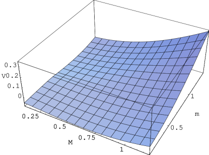
FIG. 5.: Phase Coexistence Effective Potential at $T=0.02,\mu=0.56,\delta={1\over 4\pi}$

FIG. 6.: Phase Coexistence Effective Potential as a function of $M$ for $m=0$

FIG. 7.: Phase Coexistence Effective Potential as a function of $m$ for $M=0$

REFERENCES

- [1] K. Rajagopal, hep-ph/9908360.
- [2] D. Bailin and A. Love, Phys. Rep. 107 (1984) 325; M. Iwasaki and T. Iwado, Phys. Lett. 350B (1995) 163; M. Alford, K. Rajagopal and F. Wilczek, Phys. Lett. 422B (1998) 247; R. Rapp, T. Schäfer, E.V. Shuryak and M. Velkovsky, Phys. Rev. Lett. 81 (1998) 53.
- [3] M. Alford, K. Rajagopal and F. Wilczek, Nucl. Phys. A638, 515c (1998) and Nucl. Phys. B537, 443 (1999); J. Berges and K. Rajagopal, Nucl. Phys. B538, 215 (1999); T. Schäfer, Nucl. Phys. A642, 45 (1998); T. Schäfer and F. Wilczek, Phys. Rev. Lett. 82, 3956 (1999).
- [4] N. Evans, S.D.H. Hsu and M. Schwetz, hep-ph/9808444 and Phys. Lett. B449, 281 (1999); T. Schäfer and F. Wilczek, Phys. Lett. B450, 325 (1999).
- [5] R. Pisarski and F. Wilczek, Phys. Rev. D29 338, (1984).
- [6] A. Barducci, R. Casalbuoni, G. Pettini, and R. Gatto, Phys. Rev.D 49, 426 (1994).
- [7] F. Cooper, Y. Kluger and E. Mottola Phys. Rev. C54 3298 (1996) hep-ph/9604284. M. Kennedy,J. Dawson and F. Cooper Phys.Rev.D54 2213, (1996). hep-th/9603068
- [8] D.J. Gross and A. Neveu, Phys. Rev. D10 (1974) 3235.
- [9] A. Chodos, H. Minakata and F. Cooper, Phys. Lett. B449, 260 (1999).
- [10] U. Wolff, Phys. Lett. B 157, 303 (1985); L. Jacobs, Phys. Rev. D10 (1974) 3956; B. Harrington and A. Yildiz, Phys. Rev. D11 (1975) 779.
- [11] A. Chodos and H. Minakata, Phys. Lett. A191, 39 (1994); Nucl. Phys. B 490, 687 (1997).
- [12] J. Hubbard, Phys. Rev. Lett. 3, 77 (1959); R.L. Stratonovich, Doklady Akad. Nauk. SSSR 115, 1097 (1957); S. Coleman, Aspects of Symmetry, Cambridge Press, 1985, p. 354.
- [13] S. Coleman, Comm. Math. Phys. 31 (1973) 259; N.D. Mermin and H. Wagner, Phys. Rev. Lett. 17 (1966) 1133.
- [14] E. Witten, Nucl. Phys. B145 (1978) 110.
- [15] Howard Haber and H. Arthur Weldon Phys. Rev D 25, 502 (1982)
- [16] T. Inagaki, in Proceedings of the 4th Workshop on Thermal Field Theories and their Applications, Dalian, China, 1995, pp. 121-130 (hep-ph 9511201).
- [17] I. Ojima and R. Fukuda, Research Institute for Fundamental Physics Preprint RIFP-267 (October 1976 Unpublished).
- [18] One first computes dV/dM, then expands the integral asymptotically in M/T, and then integrates on M. The relevant expansion is given in L. Dolan and R. Jackiw, Phys. Rev. D9, 3320 (1974), eqs. (C13) and (C16).