Physics Beyond the Standard Model

Abstract

These lectures describe why one believes there is physics beyond the Standard Model and review the expectations of three alternative explanations for the Fermi scale. After examining constraints and hints for beyond the Standard Model physics coming from experiment, I discuss, in turn, dynamical symmetry breaking, supersymmetry and extra compact dimension scenarios associated with the electroweak breakdown.

1 Introduction

The Standard Model (SM), $\!{}^{{\bf?}}$ gives an excellent theoretical description of the strong and electroweak interactions. This theory, which is based on an $SU(3)\times SU(2)\times U(1)$ gauge group, has proven extraordinarily robust. As shown in Fig. 1, all data in the electroweak sector to date appears to be in perfect agreement with the SM predictions, and there are just a few (quite indirect) hints for physics beyond the SM. Nevertheless, there are theoretical aspects of the SM which suggest the need for new physics. In addition, there are certain open questions within the SM whose answers can only be found by invoking physics beyond the SM.

In the last year, the observation by the SuperKamiokande $\!{}^{{\bf?}}$ collaboration of neutrino oscillations provided the first experimental indication that some new physics exists which causes a large splitting among the leptonic doublets. While in the quark sector $m_{u}/m_{d}\sim O(1)$, it appears that in the leptonic sector $m_{\nu_{\ell}}/m_{\ell}\leq 10^{-8}$. As we shall see, the most natural explanation for this phenomena is the existence of a new scale far above the electroweak scale.

In these Lectures I will try to explore some of the new physics scenarios which are motivated by theoretical considerations and try to confront and constrain them with what we know experimentally, both from the indirect hints coming from the electroweak sector as well as from the more direct hints coming from neutrino oscillations.

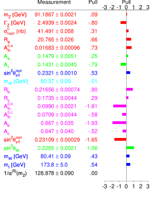
Figure 1: Standard Model fit, from Ref.2.

2 Theoretical Issues in the Standard Model

The Standard Model Lagrangian can be written as the sum of four pieces. Schematically, one has

$${\cal{L}}_{\rm SM}=-\sum_{f}\bar{\psi}_{f}\gamma^{\mu}\frac{1}{i}D_{\mu}\psi_{f}-\frac{1}{4}\sum_{i}F_{i}^{\mu\nu}F_{i\mu\nu}+{\cal{L}}_{\rm SB}+{\cal{L}}_{\rm Yukawa}~{}.$$ (1)

The first two terms in the above Lagrangian contain the interactions of the fermions in the theory with the gauge fields and the self-interactions of the gauge fields. The precision electroweak measurements, as well as most QCD tests, essentially have checked these pieces of the SM. In fact, for the electroweak tests, all that the symmetry-breaking piece, ${\cal{L}}_{\rm SB}$ and the Yukawa piece, ${\cal{L}}_{\rm Yukawa}$, provide are a renormalizable cut-off $M_{H}$ and a large fermion mass $m_{t}$, respectively. Of course, ${\cal{L}}_{\rm SB}$ also allows for the spontaneous generation of mass for the $W$ and $Z$ bosons. The masses of these excitations are given by the formulas

$$M^{2}_{W}=\frac{1}{4}g^{2}v_{F}^{2}~{};~{}~{}M^{2}_{Z}=\frac{1}{4}(g^{2}+g^{\prime 2})v_{F}^{2}$$ (2)

which involve the $SU(2)[g\equiv g_{2}]$, and $U(1)[g^{\prime}]$, coupling constants as well as a mass scale, $v_{F}$, arising from ${\cal{L}}_{\rm SB}$. This scale—the Fermi scale—is related to the Fermi constant $G_{F}$ and sets the scale of the electroweak interactions:

$$v_{F}=(\sqrt{2}G_{F})^{-1/2}\simeq 250~{}{\rm GeV}~{}.$$ (3)

It is important to note that neither the pure gauge field piece of ${\cal{L}}_{\rm SM}$ nor the fermion-gauge piece of this Lagrangian contain explicit mass terms. A mass term for the gauge fields

$${\cal{L}}_{\rm mass}^{\rm Gauge}=-\frac{1}{2}\sum_{i}m^{2}_{i}A^{\mu}_{i}A_{\mu i}$$ (4)

is forbidden explicitly by the local $SU(3)\times SU(2)\times U(1)$ symmetry. However, masses for the gauge fields [cf. Eq. (2)] can arise after the symmetry breakdown $SU(2)\times U(1)\to U(1)_{\rm em}$. Similarly, fermion mass terms of the form

$${\cal{L}}_{\rm mass}^{\rm Fermions}=-\sum_{f}m_{f}(\bar{\psi}_{f{\rm L}}\psi_{f{\rm R}}+\bar{\psi}_{f{\rm R}}\psi_{f{\rm L}})$$ (5)

are forbidden by the $SU(2)\times U(1)$ assignments of the fermions. This follows since all left-handed fermions are part of $SU(2)$ doublets, while all right-handed fermions are $SU(2)$ singlets.

Because of these circumstances, mass generation in the Standard Model is intimately connected to the spontaneous breakdown of the electroweak $SU(2)\times U(1)$ symmetry. As a result, not only are the gauge boson masses $M_{W}$ and $M_{Z}$ proportional to the Fermi scale $v_{F}$, but so are the masses for all the fermions as well as the mass of the Higgs boson $H$

$$m_{f}\sim v_{F}~{};~{}~{}~{}M_{H}\sim v_{F}~{}.$$ (6)

The difference between Eq. (2) and Eq. (6) is that, in the latter case, the proportionality constants are not known. Or, better said, they are related to phenomena we have not yet seen.

There are, however, two important exceptions to the pattern given by Eq. (6). First of all, the masses of hadrons are not simply related to the masses of quarks. Thus they depend on another scale besides $v_{F}$. This scale, $\Lambda_{\rm QCD}$, is a dynamical scale whose magnitude can be inferred from the running of the $SU(3)$ coupling constant. A convenient definition is to take $\Lambda_{\rm QCD}$ to be the scale where $\alpha_{3}(q^{2})=g^{2}_{3}(q^{2})/4\pi$ becomes of $O(1)$. Then $\Lambda_{\rm QCD}$ serves to set the mass scale of the light hadrons which receive the bulk of their mass from QCD dynamical effects. Hadrons containing heavy quarks, on the other hand, get most of their mass from the mass of the heavy quark. Thus, less of their mass depends on QCD dynamics and $\Lambda_{\rm QCD}$.

The second exception to Eq. (6) is provided by neutrinos. It is clear that for any particle carrying electromagnetic charge the only allowed mass term must involve particles and antiparticles, as detailed in Eq. (5). Lorentz invariance, however, allows one to write down mass terms involving two particle fields, or two antiparticle fields. Such mass terms, called Majorana mass terms, are allowed for neutrinos. In particular, since the right-handed neutrinos have no $SU(2)\times U(1)$ quantum numbers, one can write down an $SU(2)\times U(1)$ invariant mass term for these states of the form

$${\cal{L}}_{\rm mass}^{\rm Majorana}=-\frac{1}{2}(\nu_{\rm R}^{T}M_{\rm R}\tilde{C}\nu_{\rm R}+\bar{\nu}_{\rm R}\tilde{c}M_{\rm R}^{\dagger}\bar{\nu}_{\rm R}^{T})~{}.$$ (7)

Here $\tilde{C}$ is a charge conjugation matrix needed for Lorentz invariance.$\!{}^{{\bf?}}$ The right-handed neutrino mass matrix $M_{\rm R}$ contains mass scales which are totally independent from $v_{F}$. We will return to this point later on in these lectures.

Ignoring these more detailed questions, one of the principal issues which remains open in the Standard Model is the nature of the Fermi scale $v_{F}$. The role of symmetry breakdown as a generator of mass scales is familiar in superconductivity. In that case, the formation of an electron number violating Cooper pair $\langle e^{\uparrow}e^{\downarrow}\rangle$ $\!{}^{{\bf?}}$ sets up a mass gap between the normal and the superconducting ground states. The Fermi scale $v_{F}$ plays an analogous role in the electroweak theory. It is the scale of the order parameter which is responsible for the breakdown of $SU(2)\times U(1)$ down to $U(1)_{\rm em}$.

Although the size of $v_{F}$ $(v_{F}\sim 250~{}{\rm GeV})$ is known, its precise origin is yet unclear. Two possibilities have been suggested for the origin of $v_{F}$:

i) The Fermi scale is associated with the vacuum expectation value (VEV) of some elementary scalar field, or fields $\langle\Phi_{i}\rangle$.

ii) The Fermi scale is connected with the formation of some dynamical condensates of fermions of some underlying deeper theory, $\langle\bar{F}F\rangle$.

Roughly speaking, the above two alternatives correspond to having ${\cal{L}}_{\rm SB}$ being described either by a weakly coupled theory or by a strongly coupled theory.

The nature and origin of the Fermi scale, of course, is not the only unanswered theoretical question in the SM. Equally mysterious is the physics which gives rise to ${\cal{L}}_{\rm Yukawa}$—the piece of the SM Lagrangian which is responsible for the masses of, and mixing among, the elementary fermions in the theory. In contrast to $v_{F}$, however, here one does not have directly a scale to associate with this Lagrangian. It could well be that the flavor problem—the origin of the fermion masses and of fermion mixing—is the result of physics operating at scales which are much larger than $v_{F}$. Indeed, as we will see, trying to generate ${\cal{L}}_{\rm Yukawa}$ itself from physics at a scale of order $v_{F}$ is fraught with difficulties.

In view of the above, I will concentrate for now on only on the symmetry breaking piece of the SM Lagrangian. In this context, it proves useful to begin by examining the simplest example of ${\cal{L}}_{\rm SB}$ in which this Lagrangian involves just one complex doublet Higgs field: $\Phi=\left(\begin{array}[]{c}\phi^{o}\\ \phi^{-}\end{array}\right)$:

$${\cal{L}}_{\rm SB}=-(D_{\mu}\Phi)^{\dagger}(D^{\mu}\Phi)-\lambda\left[\Phi^{\dagger}\Phi-\frac{1}{2}v_{F}^{2}\right]^{2}~{}.$$ (8)

In the above $\lambda$ is an, arbitrary, coupling constant which, however, must be positive to guarantee a positive definite Hamiltonian.

The Fermi scale $v_{F}$ enters directly as a scale parameter in the Higgs potential

$$V=\lambda\left[\Phi^{\dagger}\Phi-\frac{1}{2}v_{F}^{2}\right]^{2}~{}.$$ (9)

The sign in front of the $v_{F}^{2}$ term is chosen appropriately to guarantee that $V$ will be asymmetric, with a minimum at a non-zero value for $\Phi^{\dagger}\Phi$. This fact is what triggers the breakdown of $SU(2)\times U(1)$ to $U(1)_{\rm em}$, since it forces the field $\Phi$ to develop a non-zero VEV.

$$\langle\Phi\rangle=\frac{1}{\sqrt{2}}\left(\begin{array}[]{c}v_{F}\\ 0\end{array}\right)~{}.$$ (10)

Because $v_{F}$ is an internal scale in the potential $V$, in isolation, it clearly makes no sense to ask what physics fixes the scale of $v_{F}$ to be any given particular number. This question, however, can be asked if one considers the SM in a larger context. For instance, one can imagine that the SM is an effective theory valid up to some very high cut-off scale $\Lambda$, where new physics comes in. An obvious candidate for $\Lambda$ is the Planck scale $M_{P}\sim 10^{19}~{}{\rm GeV}$, the scale associated with gravity, embodied in Newton’s constant $G_{N}=\frac{1}{M_{P}^{2}}$. In this broader context then it makes sense to ask what is the relation of $v_{F}$ to the cut-off $\Lambda$. In fact, because the $\lambda\Phi^{4}$ theory is trivial, $\!{}^{{\bf?}}$ with the only consistent theory being one where $\lambda_{\rm ren}\to 0$, considering the scalar interactions in ${\cal{L}}_{\rm SB}$ without some high energy cut-off is not sensible. Let me explain.

One can readily compute the evolution of the coupling constant $\lambda$ as a function of $q^{2}$. One finds that $\lambda(q^{2})$ evolves in an opposite way to the way in which the QCD coupling constant $\alpha_{3}(q^{2})$ evolves, growing as $q^{2}$ gets larger. This can be seen immediately from the Renormalization Group equation (RGE) for $\lambda$

$$\frac{d\lambda}{d\ln q^{2}}=+\frac{3}{4\pi^{2}}\lambda^{2}+\ldots$$ (11)

This equation, in contrast to the QCD case, has a positive rather than a negative sign in front of its first term. As a result, if one solves the above RGE, including only this first term, one finds a singularity at large $q^{2}$ which is a reflection of this growth

$$\lambda(q^{2})=\frac{\lambda(\Lambda_{o}^{2})}{1-\frac{3\lambda(\Lambda_{o}^{2})}{4\pi}\ln\frac{q^{2}}{\Lambda_{o}^{2}}}~{}.$$ (12)

This singularity is known as the Landau pole, since Landau was the first to notice this anomalous kind of behavior.$\!{}^{{\bf?}}$

One cannot really trust the location of the Landau pole derived from Eq. (12)

$$\Lambda_{c}^{2}=\Lambda_{o}^{2}\exp\left[\frac{4\pi^{2}}{3\lambda(\Lambda_{o}^{2})}\right]~{},$$ (13)

since Eq. (12) stops being valid when $\lambda$ gets too large. When this happens, of course, one should not have neglected the higher order terms in Eq. (11). Nevertheless, once the cut-off $\Lambda_{c}$ is fixed, one can predict $\lambda(q^{2})$ for scales $q^{2}$ sufficiently below the cut-off. Indeed, the $\lambda\Phi^{4}$ theory is perfectly sensible as long as one restricts oneself to $q^{2}\ll\Lambda_{c}^{2}$. If one wants to push the cut-off to infinity, however, one sees from (13) that $\lambda(\Lambda_{o}^{2})\to 0$. This is the statement of triviality, $\!{}^{{\bf?}}$ within this simplified context.

In the case of the SM, one can “measure” where the cut-off $\Lambda_{c}$ is in ${\cal{L}}_{\rm SB}$ from the value of the Higgs mass. Using the potential (9) one finds that

$$M_{H}^{2}=2\lambda(M_{H}^{2})v_{F}^{2}~{}.$$ (14)

Obviously, as long as the Higgs mass is light with respect to $v_{F}$ the coupling $\lambda$ is small and the cut-off is far away. Indeed, using Eqs. (13) and (14) one finds that even if $M_{H}\sim 200~{}{\rm GeV}$, then the cut-off is very large still, of order of the Planck mass $\Lambda_{c}\sim M_{P}$! So, as long as $M_{H}$ is that light, or lighter, the effective theory described by ${\cal{L}}_{\rm SB}$ is very reliable, and weakly coupled, with $\lambda\leq 0.3$. In these circumstances it is meaningful to ask the question whether the large hierarchy

$$v_{F}\ll\Lambda_{c}$$ (15)

is a stable condition. This question, following ’t Hooft, $\!{}^{{\bf?}}$ is often called the problem of naturalness.

If, on the other hand, the Higgs mass is heavy, of order of the cut-off $(M_{H}\sim\Lambda_{c})$, then it is pretty clear that ${\cal{L}}_{\rm SB}$ as an effective theory stops making sense. The coupling $\lambda$ is so strong that one cannot separate the particle-like excitations from the cut-off itself. Numerical investigations on the lattice $\!{}^{{\bf?}}$ have indicated that this occurs when

$$M_{H}\sim\Lambda_{c}\sim 700~{}{\rm GeV}~{}.$$ (16)

In this case, it is clear that $\langle\Phi\rangle$, as the order parameter of the symmetry breakdown, must be replaced by something else.

Before discussing this latter point, let me first return to the light Higgs case. Here one must worry about the naturalness of having the Fermi scale $v_{F}$ be so much smaller that the Planck mass $M_{P}$, which is clearly a physical cut-off. It turns out, in general, that the hierarchy $v_{F}\ll M_{P}$ is not stable. This is easy to see since radiative effects in a theory with a cut-off destabilize any pre-existing hierarchy. Indeed, this was ’t Hooft’s original argument.$\!{}^{{\bf?}}$ Quantities that are not protected by symmetries suffer quadratic mass shifts. This is the case for the Higgs mass. This mass, schematically, shifts from the value given in Eq. (14) to

$$M_{H}^{2}=2\lambda v_{F}^{2}+\alpha\Lambda_{c}^{2}~{}.$$ (17)

It follows from Eq. (17) that if $\Lambda_{c}\sim M_{P}\gg v_{F}$, the Higgs bosons cannot remain light. Or, saying it another way, if one wants the Higgs to remain light, one needs an enormous amount of fine tuning of parameters to guarantee that, in the end, it remains a light excitation. This kind of fine-tuning is really unacceptable, so one is invited to look for some protective symmetry to guarantee that the hierarchy $v_{F}\ll M_{P}$ is stable.

Such a protective symmetry exists—it is supersymmetry (SUSY).$\!{}^{{\bf?}}$ SUSY is a boson-fermion symmetry in which bosonic degrees of freedom are paired with fermionic degrees of freedom. If supersymmetry is exact then the masses of the fermions and of their bosonic partners are the same. In a supersymmetric version of the Standard Model all quadratic divergences cancel. Thus parameters like the Higgs boson mass will not be sensitive to a high energy cut-off. Roughly speaking, via supersymmetry, the Higgs boson mass is kept light naturally since its fermionic partner has a mass which is protected by a chiral symmetry and is of $O(v_{F})$.

Because one has not seen any of the SUSY partners of the states in the SM yet, it is clear that if a supersymmetric extension of the SM exists then the associated supersymmetry must be broken. Remarkably, even if SUSY is broken the naturalness problem in the SM is resolved, provided that the splitting between the fermion-boson SUSY partners is itself of $O(v_{F})$. For example, the quadratic divergence of the Higgs mass due to a $W$-loop is moderated into only a logarithmic divergence by the presence of a loop of Winos, the spin-1/2 SUSY partners of the $W$ bosons. Schematically, in the SUSY case, Eq. (17) gets replaced by

$$M_{H}^{2}=2\lambda v_{F}^{2}+\alpha(\tilde{M}_{W}^{2}-M_{W}^{2})\ln\Lambda_{c}/v_{F}~{}.$$ (18)

So, as long as the masses of the SUSY partners (denoted by a tilde) are themselves not split away by much more than $v_{F}$, radiative corrections will not destabilize the hierarchy $v_{F}\ll\Lambda_{c}$.

Let me recapitulate. Theoretical considerations regarding the nature of the Fermi scale have brought us to consider two alternatives for new physics associated with the $SU(2)\times U(1)\to U(1)_{\rm em}$ breakdown and ${\cal{L}}_{\rm SB}$:

i) ${\cal{L}}_{\rm SB}$ is the Lagrangian of some elementary scalar fields interacting together via an asymmetric potential, whose minimum is set by the Fermi scale $v_{F}$. The presence of non-vanishing VEVs triggers the electroweak breakdown. However, to guarantee the naturalness of the hierarchy $v_{F}\ll M_{P}$, both ${\cal{L}}_{\rm SB}$ and the whole Standard Model Lagrangian must be augmented by other fields and interactions so as to enable the theory (at least approximately) to be supersymmetric. Obviously, if this alternative is true, there is plenty of new physics to be discovered, since all particles have superpartners of mass $\tilde{m}\simeq m+O(v_{F})$.

ii) The symmetry breaking sector of the SM has itself a dynamical cut-off of $O(v_{F})$. In this case, it makes no sense to describe ${\cal{L}}_{\rm SB}$ in terms of strongly coupled scalar fields. Rather, ${\cal{L}}_{\rm SB}$ describes a dynamical theory of some new strongly interacting fermions $F$, whose condensates cause the $SU(2)\times U(1)\to U(1)_{\rm em}$ breakdown. The strong interactions which form the condensates $\langle\bar{F}F\rangle\sim v_{F}^{3}$ also identify the Fermi scale as the dynamical scale of the underlying theory, very much analogous to $\Lambda_{\rm QCD}$. If this alternative turns out to be true, then one expects in the future to see lots of new physics, connected with these new strong interactions, when one probes them at energies of $O(v_{F})$.

In the past year, a third very speculative alternative has been suggested besides the two possibilities above.$\!{}^{{\bf?}}$ This alternative is based on the idea that, perhaps, in nature there could exist some extra “largish” compact dimensions of size R. $\!{}^{{\bf?}}$ In such theories, the fundamental scale of gravity in $(d+4)$-dimensions could well be quite different than the Planck scale. In particular, it may well be that

$$[M_{P}]_{d+4}\sim v_{F}~{}.$$ (19)

That is, at short distances $(r<R)$ the scale of gravity could well be different than the Planck scale, the usual scale of 4-dimensional gravity valid at large distances $(r>R)$. Indeed, this short-distance scale could be identical to the Fermi scale. The relationship between these two gravity scales depends both on $R$ and on the number of extra dimensions $d$: $\!{}^{{\bf?}}$

$$M_{P}=([M_{P}]_{d+4})^{\frac{d+2}{2}}R^{\frac{d}{2}}\sim v_{F}[v_{F}R]^{\frac{d}{2}}$$ (20)

where the second (approximate) equality holds if Eq. (19) holds.

Obviously, if Eq. (19) were to be true, then there is no naturalness issue—the Fermi scale is the scale of gravity in the “true” extra-dimensional theory! From Eq. (20) it follows that, if $d=2$, then the scale of the compact dimensions needed is quite large $R\sim 10^{-1}~{}{\rm cm}$! On the other hand, if $d=6$, as string theory suggests, then $R\sim 10^{-13}~{}{\rm cm}$. These distances are small enough that perhaps one would not have noticed the modifications implied for the gravitational potential at distances $r<R$.

Although these theories do not suffer from any naturalness problem, and thus are perfectly consistent with a single weakly-coupled Higgs field, they do predict the existence of other phenomena beyond the SM. In particular, if this alternative is correct, one would expect copious production of gravitons at energies of order $\sqrt{s}\sim v_{F}$, as one begins to excite the compact dimensions. Thus, also here there is spectacular new physics to find!

In these Lectures, I will try to illustrate some of the consequences of all the three alternatives for $v_{F}$ alluded to above. In addition, to try to divine which of the above ideas is most likely to be correct, I want to explore in some depth some of the points which come from experiment suggesting possible traces of physics beyond the Standard Model. In the next section, I will try to describe in more detail what these hints of physics beyond the Standard Model are and what is their likely origin.

3 Constraints and Hints for Beyond the Standard Model Physics

There are four different experimental inputs which help shed some light on possible physics beyond the Standard Model. I will discuss them in turn.

3.1 Implications of Standard Model Fits

One of the strongest constraints on physics beyond the SM is that the SM gives an excellent fit to the data, as we already illustrated in Fig. 1. In practice, since all fermions but the top are quite light compared to the scale of the $W$ and $Z$-bosons, all quantities in the SM are specified as functions of 5 parameters: $g$; $g^{\prime}$; $v_{F}$; $M_{H}$; and $m_{t}$. It proves convenient to trade the first three of these for another triplet of quantities in the SM which are better measured: $\alpha$; $M_{Z}$; and $G_{F}$. This trade-off has become the common practice in the field. Once one has adopted a set of standard parameters then all physical measurable quantities can be expressed as a function of this “standard set”. For example, the $W$-mass in the SM is given as a function of these parameters as:

$$\left.M_{W}\right|_{\rm SM}=M_{W}(\alpha;M_{Z};G_{F};m_{t};M_{H})~{}.$$ (21)

Because $\alpha$, $M_{Z}$, and $G_{F}$, as well as $m_{t}$ are rather accurately known, all SM fits essentially serve to constrain only one unknown–the Higgs mass $M_{H}$. This constraint, however, is not particularly strong because all radiative effects depends on $M_{H}$ only logarithmically. That is, radiative corrections give contributions of $O\left(\frac{\alpha}{\pi}\ln M_{H}/M_{Z}\right)$.

The result of the SM fit of all precision data gives for the Higgs mass the result: $\!{}^{{\bf?}}$

$$M_{H}=\left(76^{\scriptstyle+85}_{\scriptstyle-47}\right)~{}{\rm GeV}$$ (22)

or

$$M_{H}<262~{}{\rm GeV}~{}~{}(95\%~{}{\rm C.L.})~{}.$$ (23)

These results for the Higgs mass are compatible with limits on $M_{H}$ coming from direct searches for the Higgs boson in the process $e^{+}e^{-}\to ZH$ at LEP 200. The limit presented at the 1998 ICHEP in Vancouver was $\!{}^{{\bf?}}$

$$M_{H}>89.8~{}{\rm GeV}~{}~{}~{}(95\%~{}{\rm C.L.})~{}.$$ (24)

However, preliminary results presented at the 1999 Winter Conferences have raised this bound to the neighborhood of 95 GeV.

It is particularly gratifying that the SM fits indicate the need for a light Higgs boson, since this “solution” is what is internally consistent. Let me illustrate how this emerges, for example, from studies of the $Z$-leptonic vertex. The axial coupling of the $Z$

$${\cal{L}}_{\rm eff}=\frac{eZ^{\mu}}{2\cos\theta_{W}\sin\theta_{W}}\bar{e}[\gamma_{\mu}g_{V}-g_{A}\gamma_{\mu}\gamma_{5}]e$$ (25)

gets modified by radiative corrections to

$$g_{A}^{2}=\frac{1}{4}[1+\Delta\rho]~{}.$$ (26)

The shift in the $\rho$-parameter, $\Delta\rho$, gets its principal contribution from $m_{t}$. However, it has also a (weak) dependence on $M_{H}$.$\!{}^{{\bf?}}$

$$\left.\Delta\rho\right|_{\rm Higgs}=-\frac{3G_{F}M^{2}_{W}}{4\pi^{2}\sqrt{2}}\tan^{2}\theta_{W}\ln\frac{M_{H}}{M_{Z}}+\ldots\simeq-10^{-3}\ln\frac{M_{H}}{M_{Z}}~{}.$$ (27)

The SM fit gives $\!{}^{{\bf?}}$

$$\Delta\rho=(3.7\pm 1.1)\times 10^{-3}~{},$$ (28)

with the Higgs contribution giving, for $M_{H}=300$ GeV, $\Delta\rho=-1\times 10^{-3}$. Obviously, if $M_{H}$ were to be very large, the Higgs contribution could have even changed the sign of $\Delta\rho$. The value emerging from the SM fit instead is perfectly compatible with having a rather light Higgs mass. In fact, one nice way to summarize the result of the SM fit is that, approximately, this fit constrains

$$\ln\frac{M_{H}}{M_{Z}}\leq 1~{}.$$ (29)

That is, there are no large logarithms associated with the symmetry breaking sector.

I should remark that a good SM fit does not necessarily exclude possible extensions of the SM involving either new particles or new interactions, provided that these new particles and/or interactions give only small effects. Typically, the effects of new physics are small if the excitations associated with this new physics have mass scales several times the $W$-mass.

One can quantify the above discussion in a more precise way by introducing a general parametrization for the vacuum polarization tensors of the gauge bosons and the $Zb\bar{b}$ vertex. These are the places where the dominant electroweak radiative corrections occur and therefore are the quantities which are probably the most sensitive new physics.$\!{}^{{\bf?}}$ I do not want to enter into a full discussion of this procedure here since it is already well explained in the literature.$\!{}^{{\bf?}}$ However, I want to talk about one example, connected to modifications of the gauge fields vacuum polarization tensors, because precision electroweak data serves to provide a strong constraint on dynamical symmetry breaking theories-excluding theories which are QCD-like.

There are four distinct vacuum polarization contributions $\Sigma_{AB}(q^{2})$, where the pairs $AB=\{ZZ,WW,\gamma\gamma,\gamma Z\}$. For sufficiently low values of the momentum transfer $q^{2}~{}(q^{2}\simeq M^{2}_{W})$ it obviously suffices to expand $\Sigma_{AB}(q^{2})$ only up to $O(q^{2})$. Thus, approximately, one needs to consider 8 different parameters associated with these contributions:

$$\Sigma_{AB}(q^{2})=\Sigma_{AB}(0)+q^{2}\Sigma_{AB}^{\prime}(0)+\ldots~{},$$ (30)

with the remaining corrections being terms of $O\left(\frac{q^{4}}{\Lambda^{2}}\right)$ with $\Lambda$ being the scale of the new physics. In fact, there are not really 8 independent parameters since electromagnetic gauge invariance requires that

$$\Sigma_{\gamma\gamma}(0)=\Sigma_{\gamma Z}(0)=0~{}.$$ (31)

Of the 6 remaining parameters one can fix 3 combinations of coefficients in terms of $G_{F},~{}\alpha$ and $M_{Z}$. Hence, in a most general analysis, the gauge field vacuum polarization tensors (for $q^{2}\stackrel{{\scriptstyle<}}{{{}_{\scriptstyle\sim}}}M_{W}^{2}$) only involve 3 arbitrary parameters. The usual choice,$\!{}^{{\bf?}}$ is to have one of these contain the main quadratic $m_{t}$-dependence, leaving the other two essentially independent of $m_{t}$.

I will proceed with my discussion in terms of the parametrization of Altarelli and Barbieri,$\!{}^{{\bf?}}$ where these three parameters are chosen to be

$$\epsilon_{1} = \Delta\rho=\left[\frac{\Sigma_{ZZ}(0)}{M^{2}_{Z}}-\frac{\Sigma_{WW}(0)}{M^{2}_{W}}\right]\stackrel{{\scriptstyle\rm SM}}{{=}}\frac{3G_{F}m_{t}^{2}}{8\pi^{2}\sqrt{2}}-\frac{3G_{F}M^{2}_{W}}{4\pi^{2}\sqrt{2}}\tan^{2}\theta_{W}\ln\frac{M_{H}}{M_{Z}}\ldots$$ (32)

$$\epsilon_{2} = \left[\Sigma^{\prime}_{11}(0)-\Sigma^{\prime}_{33}(0)\right]\stackrel{{\scriptstyle\rm SM}}{{=}}-\frac{G_{F}M^{2}_{W}}{2\pi^{2}\sqrt{2}}\ln\frac{m_{t}}{M_{Z}}+\ldots$$ (33)

$$\epsilon_{3} = \left[\Sigma^{\prime}_{3\gamma}(0)-\Sigma^{\prime}_{3Z}(0)\right]\stackrel{{\scriptstyle\rm SM}}{{=}}\frac{G_{F}M^{2}_{W}}{12\pi^{2}\sqrt{2}}\ln\frac{M_{H}}{M_{Z}}-\frac{G_{F}M^{2}_{W}}{6\pi^{2}\sqrt{2}}\ln\frac{m_{t}}{M_{Z}}+\ldots$$ (34)

Here, as usual, $Z=3-\sin^{2}\theta_{W}\gamma$ and $W^{\pm}={1\over\sqrt{2}}[1\mp i2]$. In the above, I have displayed also the leading dependence on $m_{t}$ and $M_{H}$ of the $\epsilon_{i}$ in the SM.

The interesting parameter here is $\epsilon_{3}$, whose experimental value turns out to be $\!{}^{{\bf?}}$

$$\epsilon_{3}=(3.9\pm 1.1)\times 10^{-3}~{}.$$ (35)

One can estimate $\epsilon_{3}$ in a dynamical symmetry breaking theory, if one assumes that the spectrum of such a theory, and its dynamics, is QCD-like.$\!{}^{{\bf?}}$ From its definition, one sees that $\epsilon_{3}$ involves the difference between the spectral functions of vector and axial vector currents

$$\epsilon_{3}=\frac{1}{2}\left[\Sigma^{\prime}_{VV}(0)-\Sigma^{\prime}_{AA}(0)\right]~{}.$$ (36)

This difference has two components in a dynamical symmetry breaking theory. There is a contribution from a heavy Higgs boson $(M_{H}\sim{\rm TeV})$ characteristic of such theories, plus a term detailing the differences between the vector and axial vector spectral functions. This second component reflects the resonances with these quantum numbers in the spectrum of the underlying theory which gives rise to the symmetry breakdown. The first piece is readily estimated from the SM expression, using $M_{H}\sim{\rm TeV}$. The second piece, in a QCD-like theory, can be deduced by analogy to QCD, modulo some counting factors associated with the type of underlying theory one is considering. One finds $\!{}^{{\bf?}}$

$$\epsilon_{3} = \left.\epsilon_{3}\right|_{M_{H}\simeq 1~{}{\rm TeV}}+\frac{\alpha}{12\pi\sin^{2}\theta_{W}}\int^{\infty}_{0}\frac{ds}{s}[R_{V}(s)-R_{A}(s)]$$ (37)

$$= 6.65\times 10^{-3}+N_{D}\left(\frac{N_{TC}}{4}\right)\left[\frac{2\alpha\pi}{\sin^{2}\theta_{W}}\frac{f_{\pi}^{2}}{m_{\rho}^{2}}\right]$$

$$= \left[6.65\pm 3.4N_{D}\left(\frac{N_{TC}}{4}\right)\right]\times 10^{-3}~{}.$$

The second line above follows if the underlying theory is QCD-like, so that the resonance spectrum is saturated by $\rho$-like and $A_{1}$-like, resonances. Here $N_{D}$ is the number of doublets entering in the underlying theory and $N_{TC}$ is the number of “Technicolors” in this theory. Using Eq. (34) and using $N_{TC}=4$, as is usually assumed, one sees that

$$\epsilon_{3}=\left\{\begin{array}[]{ll}10.05\times 10^{-3}&N_{D}=1\\ 20.25\times 10^{-3}&N_{D}=4\end{array}\right.$$ (38)

These values for $\epsilon_{3}$ are, respectively, $5.5\sigma$ and $15\sigma$ away from the best fit value of $\epsilon_{3}$, obtained from fitting all the high precision electroweak data. Obviously, one cannot countenance anymore a dynamical symmetry breaking theory which is QCD-like!

Provided the superpartners are not too light, nothing as disastrous occurs instead if one considers a supersymmetric extension of the SM. Fig. 2, taken from a recent analysis of Altarelli, Barbieri, and Caravaglios,$\!{}^{{\bf?}}$ shows a typical fit, scanning over a range of parameters in the MSSM—the minimal supersymmetric extension of the SM. Although the MSSM can improve the $\chi^{2}$ of the fit over that for the SM (which is already very good!), these improvements are small. In effect, the MSSM radiative corrections fits are all slightly better than the SM fits. This is not surprising, since these latter fits contain more parameters. Interestingly, however, these fits do not provide better bounds on sparticles than the bounds obtained by direct searches. Of course, for certain cases there are constraints. For instance, there cannot be too large a stop-sbottom splitting because such a splitting would give too large a value for $\epsilon_{1}=\Delta\rho$.

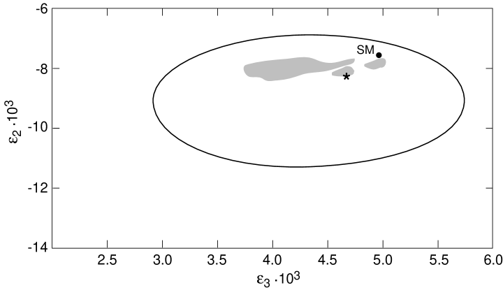
Figure 2: Comparison of SM and MSSM fits in the $\epsilon_{2}-\epsilon_{3}$ plane, from Ref.20. The ellipse is the 1-$\sigma$ range determined by the data. The shaded region is the result of a scan over a range of SUSY parameters, with the star marking the lowest $\chi^{2}$ point.

3.2 Hints of Unification

Although the SM coupling constants are very different at energies of order of the Fermi scale, these couplings can become comparable at very high energies because they evolve differently with $q^{2}$. $\!{}^{{\bf?}}$ Indeed, it is quite possible that the SM couplings unify into a single coupling at high energy, reflecting an underlying Grand Unified Theory (GUT) which breaks down to the SM at a high scale. If $G$ denotes the GUT group, then one can imagine the sequence of spontaneous breakings

$$G\stackrel{{\scriptstyle M_{X}}}{{\longrightarrow}}SU(3)\times SU(2)\times U(1)\stackrel{{\scriptstyle v_{F}}}{{\longrightarrow}}SU(3)\times U(1)_{\rm em}~{},$$ (39)

with $M_{X}\gg v_{F}$.

To test this assumption one can compute the evolution of the SM coupling constants using the Renormalization Group Equations (RGE) and see if, indeed, these coupling constants unify. To leading order, the evolution of each coupling constant can be evaluated separately from the others, since they decouple from each other:

$$\frac{d\alpha_{i}(\mu^{2})}{d\ln\mu^{2}}=-\frac{b_{i}}{4\pi}\alpha_{i}^{2}(\mu^{2})~{}.$$ (40)

These equations imply a logarithmic change for the inverse couplings

$$\alpha_{i}^{-1}(q^{2})=\alpha_{i}^{-1}(M^{2})+\frac{b_{i}}{4\pi}\ln\frac{q^{2}}{M^{2}}~{}.$$ (41)

The rate of change of the coupling constants with energy is governed by the coefficients $b_{i}$ which enter in the RGE. In turn, these coefficients depend on the matter content of the theory—which matter states are “active” at the scale one is probing. In general, one has $\!{}^{{\bf?}}$

$$b_{i}=\sum_{\rm states}\left\{\frac{11}{6}\ell_{i}^{\rm vector}-\frac{1}{3}\ell_{i}^{\rm chiral~{}fermion}-\frac{1}{12}\ell_{i}^{\rm real~{}scalar}\right\}$$ (42)

with the $\ell_{i}$ being group theoretic factors. For $SU(N)$ groups $\!{}^{{\bf?}}$ $[\ell_{i}]_{\rm Adjoint}=2N$, while for fields transforming according to the fundamental representation, $[\ell_{i}]_{\rm Fundamental}=1$. For $U(1)$ groups, $\ell_{i}=2Q^{2}$, where $Q$ is a “property normalized” charge. That is, a charge which allows the possibility of unifying the $U(1)$ groups with the other non-Abelian groups. Let me explain this last point further.

For non-Abelian groups, the generators in the fundamental representation are conventionally normalized $\!{}^{{\bf?}}$ so that

$${\rm Tr}~{}t_{a}t_{b}=\frac{1}{2}\delta_{ab}~{}.$$ (43)

For Abelian groups one can always rescale the charge. Thus no similar convention exists for this case. For example, for the electroweak group, instead of the usual hypercharge $Y$, one can define a new charge $Q$ related to $Y$ by a constant:

$$Y=\xi Q~{}.$$ (44)

Obviously, the conventional hypercharge coupling can be turned into a $Q$-coupling, by rescaling the $U(1)$ coupling constant:

$$g^{\prime}Y=g^{\prime}\xi Q=g_{1}Q~{}.$$ (45)

For unification, one wants a $U(1)$ charge that is normalized in the same way as the non-Abelian generators, when one sweeps over all quarks and leptons

$$\sum_{q+\ell}{\rm Tr}~{}t_{a}^{2}=\sum_{q+\ell}{\rm Tr}~{}Q^{2}\equiv\frac{1}{\xi^{2}}\sum_{q+\ell}{\rm Tr}~{}Y^{2}~{}.$$ (46)

Because $\displaystyle{\sum_{q+\ell}}{\rm Tr}~{}t_{a}^{2}=2$, while $\displaystyle{\sum_{q+\ell}}{\rm Tr}~{}Y^{2}=10/3$ it follows that $\xi=\sqrt{5/3}$. So,

$$Q=\sqrt{\frac{3}{5}}Y~{};~{}~{}~{}g_{1}=\sqrt{\frac{5}{3}}g^{\prime}~{}.$$ (47)

Using Eq. (42), it is straightforward to compute the coefficients $b_{i}$ in the SM. For example, for the QCD coupling, one finds

$$b_{3}=\left\{\frac{11}{6}\cdot 6-\frac{1}{3}\cdot 12\right\}=7~{},$$ (48)

where the first factor above is the contribution of the gluonic degree of freedom and the second factor above comes from the 6 species of left-handed quarks plus the 6 species of right-handed quarks. Obviously, if there were to be supersymmetric matter, all the coefficients $b_{i}$ would be modified at scales at or above where this matter starts to be produced. For example, in the supersymmetric QCD case, the gluons are now accompanied by spin 1/2 gluinos (which are chiral fermions) and each of the quarks of a given helicity has two real spin zero squark partners. For SUSY QCD then, the coefficient $b_{3}$ becomes

$$b_{3}=\left\{\frac{11}{6}\cdot 6-\frac{1}{3}\cdot 12-\frac{1}{3}\cdot 6-\frac{1}{12}\cdot 24\right\}=3~{}.$$ (49)

Table 1 compares the predictions for the coefficients $b_{i}$ of the SM and the SUSY extension.

Table 1: Coefficients $b_{i}$ in the SM and in the SUSY SM

Coefficient	SM	SUSY SM
$b_{1}$	$-41/10$	$-33/5$
$b_{2}$	$+19/6$	$-1$
$b_{3}$	$+7$	$+3$

Using the result of this table, along with input data for $\alpha_{i}(M^{2}_{Z})$ $\!{}^{{\bf?}}$, one can compute the evolution of the coupling constants in both models. $\!{}^{{\bf?}}$ As is shown in Fig. 3, for the SM there is a near unification of the couplings around $M_{X}\simeq 10^{15}$ GeV. However, rather remarkably, in the supersymmetric extension of the SM, the presence of the SUSY matter, by altering the evolution, appears to give a true unification of the coupling constants at $M_{X}\simeq 10^{16}$ GeV.

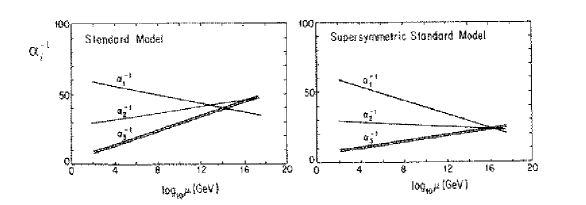
Figure 3: Evolution of couplings without and with SUSY matter.

The unification of the couplings in the SUSY SM case is quite spectacular. However, per se, this is only suggestive. It is not either a “proof” that a low energy supersymmetry exists, nor does it mean that there exists some high energy GUT! The proof of the former really requires the discovery of the predicted SUSY partners, while for GUTs one must find typical phenomena which are associated with these theories–like proton decay. This said, however, one can gather additional ammunition in favor of this picture from some of the properties of the top quark. I turn to this point next.

3.3 Implications of a Large Top Mass

Of all the quarks and leptons, only top has a mass which is of order of the Fermi scale, $v_{F}\simeq 250$ GeV. In this sense, top is unique among all the fundamental particles, since it has a mass whose value is basically set by the value of the order parameter responsible for the electroweak breakdown: $m_{t}\sim v_{F}$. All other elementary excitations are related to $v_{F}$ by constants which are much less than unity.

If one is permitted a perturbative analysis, having a large top mass, in turn, gives further constraints. This is particularly true for the case of the SM, where a large top mass influences what Higgs masses are allowed. However, interesting consequences also arise in the (theoretically more pristine) SUSY SM. In both cases, rather than dealing with the “physical” top quark mass determined experimentally by CDF and DO: $\!{}^{{\bf?}}$

$$m_{t}=(173.8\pm 5.0)~{}{\rm GeV}~{},$$ (50)

it is more convenient to consider instead the running mass

$$m_{t}(m_{t})\simeq\frac{m_{t}}{1+\frac{4}{3\pi}\alpha_{3}(m_{t}^{2})}=(165\pm 5)~{}{\rm GeV}~{}.$$ (51)

This is because $m_{t}(m_{t})$ is directly related to the diagonal couplings of the top to the VEV of the Higgs boson, $H_{u}$:

$$m_{t}(m_{t})=\lambda_{t}(m_{t})\langle H_{u}\rangle~{}.$$ (52)

The Yukawa coupling $\lambda_{t}$ also obeys a RGE. Keeping only the dominant 3rd generation couplings, this equation reads: $\!{}^{{\bf?}}$

$$\frac{d\lambda_{t}(\mu)}{d\ln\mu^{2}}=\frac{1}{32\pi^{2}}\left[a_{t}\lambda_{t}^{2}(\mu)+a_{b}\lambda_{b}^{2}(\mu)+a_{\tau}\lambda_{\tau}^{2}(\mu)-4\pi c_{i}\alpha_{i}(\mu^{2})\right]\lambda_{t}(\mu)~{}.$$ (53)

Here $\lambda_{b}$ and $\lambda_{\tau}$ are, respectively, the Yukawa couplings of the $b$-quark and the $\tau$-lepton to the (corresponding) Higgs field. The coefficients $a_{t},a_{b},a_{\tau}$ and $c_{i}$ in Eq. (53) again depend on the matter content of the theory. Table 2 details them both for the SM and its SUSY extension.

Table 2: Coefficients entering the RGE for $\lambda_{t}$ for the SM and the SUSY SM

Coefficient	SM	SUSY SM
$a_{t}$	$9/2$	$6$
$a_{b}$	$3/2$	$1$
$a_{\tau}$	$1$	$0$
$c_{1}$	$17/20$	$17/5$
$c_{2}$	$9/4$	$3$
$c_{3}$	$8$	$16/3$

Because the coefficient $a_{t}>0$, it follows that also the top coupling $\lambda_{t}(\mu)$ will have a Landau pole at large values of the scale $\mu$. Of course, just as for the case of the Higgs coupling $\lambda$ discussed earlier, the location of this singularity is not to be trusted exactly since Eq. (53) breaks down in its vicinity. Nevertheless, there are significant differences between where the Landau pole for $\lambda_{t}$ is in the SM and where it is in the SUSY SM.

SM Case

Because one assumes that there is only one Higgs boson in the Standard Model, it follows that $\langle H_{u}\rangle=\frac{1}{\sqrt{2}}v_{F}\simeq 174$ GeV. This implies, in turn, a precise value for $\lambda_{t}(m_{t})$ from Eq. (52):

$$\lambda_{t}(m_{t})=0.95\pm 0.03~{}.$$ (54)

Further, since $m_{t}\gg m_{b},m_{\tau}$ and $c_{3}\alpha_{3}\gg c_{2}\alpha_{2},c_{1}\alpha_{1}$, to a good approximation the RGE (53) reduces to

$$\frac{d\lambda_{t}(\mu)}{d\ln\mu^{2}}=\frac{1}{32\pi^{2}}\left[\frac{9}{2}\lambda^{2}_{t}(\mu)-32\pi\alpha_{3}(\mu^{2})\right]\lambda_{t}(\mu)~{}.$$ (55)

Using $\alpha_{3}(m_{t}^{2})\simeq 0.118$, one sees that the above square bracket is negative at $\mu=m_{t}$. Thus in the SM, $\lambda_{t}(\mu)$ decreases as $\mu$ increases above $m_{t}$, at least temporarily. However, for very large $\mu$, eventually $\lambda_{t}(\mu)$ will begin growing and eventually it will diverge at some scale–the Landau pole.

Eq. (55) and its companion for $\alpha_{3}(\mu^{2})$, Eq. (40), can be solved in closed form. $\!{}^{{\bf?}}$ One finds for $\lambda_{t}(\mu^{2})$ the expression

$$\lambda_{t}^{2}(\mu)=\frac{\eta(\mu)\lambda_{t}^{2}(m_{t})}{\left[1-\frac{9}{16\pi^{2}}\lambda_{t}^{2}(m_{t})I(\mu)\right]}~{},$$ (56)

where the functions $\eta(\mu)$ and $I(\mu)$ contain information on the running of the strong coupling constant:

$$\eta(\mu) = \left[\frac{\alpha_{3}(m_{t}^{2})}{\alpha_{3}(\mu^{2})}\right]^{-c_{3}/b_{3}}=\left[\frac{\alpha_{3}(\mu^{2})}{\alpha_{3}(m_{t}^{2})}\right]^{8/7}$$

$$I(\mu) = \int^{\ln\mu}_{\ln m_{t}}d\ln\mu^{\prime}\eta(\mu^{\prime})$$ (57)

Using Eq. (56) it is easy to check that the Yukawa coupling $\lambda_{t}(\mu)$ decreases well beyond the Planck scale, with $\lambda_{t}(M_{\rm P})\simeq 0.65<\lambda_{t}(m_{t})$, so that the top sector is perturbative throughout the region of interest. In fact, $\lambda_{t}(\mu)$ does not begin to get large until $\mu\sim 10^{30}$ GeV, with the Landau pole occuring around $\mu=10^{32}$ GeV—scales well beyond the Planck scale.

Even though the top Yukawa coupling is below unity for $\mu<M_{\rm P}$, this coupling is large enough to affect the Higgs sector of the Standard Model. Our discussion of the Higgs self-coupling $\lambda$ in Section II was based on the RGE in which only terms involving $\lambda$ were retained. In fact, at higher order, the RGE equation for $\lambda$ is influenced both by the top Yukawa coupling and the electroweak gauge couplings. The full RGE for $\lambda$, rather than Eq. (11), reads $\!{}^{{\bf?}}$

$$\frac{d\lambda(\mu)}{d\ln\mu^{2}}=\frac{3}{4\pi^{2}}\left[\lambda^{2}(\mu)-\frac{1}{4}\lambda_{t}^{4}(\mu)+\frac{\pi}{128}[3+2\sin^{2}\theta_{W}+\sin^{4}\theta_{W}]\alpha_{2}(\mu^{2})\right]~{}.$$ (58)

The important point to notice in this equation is the negative contribution coming from the top coupling. This contribution, just like the $\alpha_{3}$ contribution in Eq. (55), can cause $\lambda(\mu)$ to decrease at first. Indeed, if the Higgs coupling $\lambda(M_{H})$ is not large enough, because the Higgs boson is light, the relatively large contribution coming from the $\lambda_{t}^{4}$ term can drive $\lambda(\mu)$ negative at some scale $\mu$. This cannot really happen physically, because for $\lambda<0$ the Higgs potential is unbounded!

To avoid this vacuum instability below some cut-off $\Lambda_{c}$–typically $\Lambda_{c}\sim M_{\rm P}$–one needs to have $\lambda(M_{H})$, and therefore the Higgs mass, sufficiently large. Hence, these considerations give a lower bound for the Higgs mass. Taking $\Lambda_{c}=M_{\rm P}$, this lower bound is $\!{}^{{\bf?}}$

$$M_{H}\geq 134~{}{\rm GeV}~{}.$$ (59)

Lowering the cut-off $\Lambda_{c}$, weakens the bound on $M_{H}$. Interestingly, to have a SM Higgs as light as 100 GeV—which is the region accessible to LEP 200—requires a very low cut-off, of order $\Lambda_{c}\sim 100$ TeV. $\!{}^{{\bf?}}$ So, finding such a Higgs may, very indirectly, point to a scenario with extra compact dimensions where such low-cut-offs are allowed. Parenthetically, I should note that these kinds of vacuum stability bounds cease to be valid in models with more than one Higgs doublet, like in the SUSY SM case.

SUSY SM

The situation is quite different for $\lambda_{t}$ if there is supersymmetric matter. Because supersymmetry necessitates two Higgs doublets, $\lambda_{t}(m_{t})$ is no longer fixed solely by the value of the top mass. The vacuum expectation values of the two Higgs bosons involve a further parameter, $\tan\beta$, besides $v_{F}$:

$$\langle H_{u}\rangle=\frac{1}{\sqrt{2}}v_{F}\sin\beta~{};~{}~{}~{}~{}\langle H_{d}\rangle=\frac{1}{\sqrt{2}}v_{F}\cos\beta~{}.$$ (60)

Thus, one has, instead of Eq. (54),

$$\lambda_{t}(m_{t})=\frac{0.95\pm 0.03}{\sin\beta}~{}.$$ (61)

Keeping again only the leading terms, the RGE for $\lambda_{t}(\mu)$ in the presence of SUSY matter reads now:

$$\frac{d\lambda_{t}(\mu)}{d\ln\mu^{2}}=\frac{1}{32\pi^{2}}\left[6\lambda_{t}^{2}(\mu)+\lambda_{b}^{2}(\mu)-\frac{64\pi}{3}\alpha_{3}(\mu^{2})\right]\lambda_{t}(\mu)~{}.$$ (62)

Because of the differrent coefficients that SUSY matter implies, it is no longer necessarily true that the square bracket above is negative at $\mu=m_{t}$, as was the case in the SM. Instead, since $64\pi\alpha_{3}(m_{t}^{2})/3\simeq 7.9$, the square bracket above can actually vanishes in two regions of parameter space. The first is the region of large $\tan\beta$ where, for large scales $\mu$, $\lambda_{b}(\mu)\simeq\lambda_{t}(\mu)\simeq 1$ [Yukawa unification region]. The second is a region where $\tan\beta\sim O(1)$, so that $\lambda_{b}(m_{t})\ll\lambda_{t}(m_{t})$, with the top contribution cancelling directly that coming from the $SU(3)$ corrections [in detail, this requires $\sin\beta=0.83\pm 0.03$].

In either of the two regions above, the presence of SUSY matter forces $\lambda_{t}$ to an infrared fixed point $\!{}^{{\bf?}}$ as $\mu$ becomes of order $m_{t}$

$$\left.\frac{d\lambda_{t}(\mu)}{d\ln\mu^{2}}\right|_{\mu\sim m_{t}}\simeq 0~{}.$$ (63)

This is a very interesting possibility, since such a condition essentially serves to drive quite different values of $\lambda_{t}(\mu)$ at high scales $\mu$ down to the same fixed point value $\lambda^{*}$, at scales $\mu\simeq m_{t}$. This behavior is illustrated in Fig. 4. Asking that Eq. (63) holds, one sees that the fixed point $\lambda^{*}$ is given by

$$\lambda^{*}=\frac{32\pi}{9}\alpha_{3}(m_{t}^{2})\left[\frac{1}{1+\frac{m_{b}^{2}(m_{t})\tan^{2}\beta}{6m_{t}^{2}(m_{t})}}\right]\simeq 1.3\left[\frac{1}{1+\frac{m_{b}^{2}(m_{t}^{2})\tan^{2}\beta}{6m_{t}^{2}(m_{t})}}\right]~{}.$$ (64)

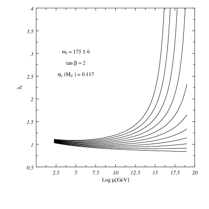
Figure 4: Focusing of the Yukawa couplings as $\lambda_{t}\to\lambda^{*}$.

Two remarks are in order

i) The fixed point behavior for $\lambda_{t}(m_{t})$ does, indeed, need supersymmetry. In the SM with only ordinary matter, one would get a fixed point behavior from the RGE for $\lambda_{t}$ only if $m_{t}$ would have been approximately 250 GeV!

ii) If one were to assume that near the Planck mass $\lambda_{t}(\mu)$ were to be large then, if there is SUSY matter, the fixed point behavior for $\lambda_{t}$ essentially serves to predict the correct value for the top mass $m_{t}(m_{t})\simeq m_{t}^{*}\simeq 170$ GeV seen by experiment.

3.4 Neutrino Oscillations

Although hints of neutrino oscillations have been around for some time, notably connected with the solar neutrino puzzle,$\!{}^{{\bf?}}$ real evidence for oscillatioins only emerged last year from data on atmospheric neutrinos studied by the large underground water Cerenkov detector, SuperKamiokande. In June 1998, the SuperKamiokande Collaboration $\!{}^{{\bf?}}$ reported a pronounced zenith angle dependence for the flux of multi-GeV atmospheric $\nu_{\mu}$ events, but no such dependence for the atmospheric $\nu_{e}$ flux. The collaboration interpreted the large up-down asymmetry seen [139 up-going $\nu_{\mu}$’s versus 256 down-going $\nu_{\mu}$’s] as evidence for $\nu_{\mu}\to\nu_{X}$ oscillations, with $\nu_{X}$ being either a $\nu_{\tau}$ or, possibly, a new sterile neutrino $\nu_{s}$.

In the usual 2-neutrino mixing formalism,$\!{}^{{\bf?}}$ the weak interaction eigenstates $|\nu_{\mu}\rangle$ and $|\nu_{X}\rangle$ are linear combinations of two mass eigenstates $|\nu_{1}\rangle$ and $|\nu_{2}\rangle$:

$$\left(\begin{array}[]{l}|\nu_{\mu}\rangle\\ |\nu_{X}\rangle\end{array}\right)=\left(\begin{array}[]{ll}\cos\theta&\sin\theta\\ -\sin\theta&\cos\theta\end{array}\right)\left(\begin{array}[]{l}|\nu_{1}\rangle\\ |\nu_{2}\rangle\end{array}\right)~{}.$$ (65)

The probability that after traversing a distance $L$ a $\nu_{\mu}$ neutrino of energy $E$ emerges as a $\nu_{X}$ neutrino is then given by the well known formula

$$P(\nu_{\mu}\to\nu_{X};L)=\sin^{2}2\theta~{}\sin^{2}\frac{\Delta m^{2}L}{4E}~{},$$ (66)

with $\Delta m^{2}=m_{2}^{2}-m_{1}^{2}$ being the difference in mass squared between the two neutrino eigenstates. From an analysis of their results, the SuperKamiokande collaboration $\!{}^{{\bf?}}$ deduced that the observed up-down asymmetry could be explained by neutrino oscillations if the mixing was nearly maximal, $\sin^{2}2\theta\simeq 1$, and if $\Delta m^{2}\simeq 2.5\times 10^{-3}~{}{\rm eV}^{2}$.

The SuperKamiokande results provide a lower bound on neutrino masses. Since

$$\Delta m^{2}=m_{2}^{2}-m_{1}^{2}\simeq 2.5\times 10^{-3}~{}{\rm eV}^{2}~{},$$ (67)

it follows that at least one neutrino has a mass larger than

$$m_{2}\geq 5\times 10^{-2}~{}{\rm eV}~{},$$ (68)

with the bound being satisfied if $m_{2}\gg m_{1}$. Such small masses, compared to the masses of quarks and leptons, suggests that new physics is at work. Indeed, the simplest way to understand why neutrinos have tiny masses is through the see-saw mechanism,$\!{}^{{\bf?}}$ which involves new physics at a scale much larger than the Fermi scale. Let me briefly discuss this reasoning.

Because neutrinos have no charge, as we remarked earlier, the most general mass term for these states can contain also particle-particle terms, besides the usual particle-antiparticle contribution. $\!{}^{{\bf?}}$ One has, considering one species of neutrinos for simplicity,

$${\cal{L}}_{\rm mass}^{\nu} = -m_{D}[\bar{\nu}_{\rm L}\nu_{\rm R}+\bar{\nu}_{\rm R}\nu_{\rm L}]-\frac{m_{\rm R}}{2}[\bar{\nu}_{\rm R}\tilde{C}\bar{\nu}_{\rm R}^{T}+\nu_{\rm R}^{T}\tilde{C}\nu_{\rm R}]$$ (69)

$$-\frac{m_{\rm L}}{2}[\nu_{\rm L}^{T}\tilde{C}\nu_{\rm L}+\bar{\nu}_{\rm L}\tilde{C}\bar{\nu}_{\rm L}^{T}]~{}.$$

In the above the different mass terms conserve/violate different symmetries. To wit:

The Dirac mass $m_{D}$: conserves lepton number L, but violates $SU(2)\times U(1)$.

The Majorana mass $m_{\rm R}$: violates lepton number L, but conserves $SU(2)\times U(1)$.

The Majorana mass $m_{\rm L}$: violates both lepton number L and $SU(2)\times U(1)$.

Because the Dirac mass term has the same form as the usual quark and lepton masses, it is sensible to imagine that $m_{D}$ should be of the same order of magnitude as these masses. Hence, schematically, one expects

$$m_{D}\sim m_{\ell}\sim v_{F}$$ (70)

where the proportionality constant to the Fermi scale may, indeed, be quite small. Thus, if one wants the physical neutrinos to have very small masses, this must be the result of the presence of the Majorana mass terms in Eq. (69).

There are two simple ways of achieving this goal, depending on whether one assumes that a right-handed neutrino $\nu_{\rm R}$ exists or not. If one does not involve a $\nu_{\rm R}$, the simplest effective interaction one can write using only $\nu_{\rm L}$ which preserves $SU(2)\times U(1)$ is $\!{}^{{\bf?}}$

$${\cal{L}}_{\rm eff}=\frac{1}{M}(\nu_{\ell}~{}\ell)_{\rm L}^{T}\tilde{C}\vec{\tau}\left(\begin{array}[]{c}\nu_{\ell}\\ \ell\end{array}\right)_{\rm L}\cdot\Phi^{T}C\vec{\tau}\Phi+{\rm h.c.}$$ (71)

Here $M$ is some, presumably large, scale which is associated with these lepton number violating processes. This term, when $SU(2)\times U(1)$ breaks down to $U(1)_{\rm em}$, generates a mass for the neutrino

$$m_{\nu}\equiv m_{\rm L}=\frac{v_{F}^{2}}{M}~{}.$$ (72)

One sees that to get neutrino masses of the order of those inferred from SuperKamiokande one requires $M\sim 10^{15}$ GeV—a scale of the order of the GUT scale!

One can get a similar result if one includes right-handed neutrinos in the theory. In this case, it is convenient to rewrite the general neutrino mass terms of Eq. (69) in terms of both neutrino fields, $\nu$, and their charged conjugate, $\nu^{c}$. Since $\!{}^{{\bf?}}$

$$\nu^{c}=\tilde{C}\bar{\nu}^{T}~{};~{}~{}~{}\overline{\nu^{c}}=\nu^{T}\tilde{C}~{},$$ (73)

Eq. (69) takes the form

$${\cal{L}}^{\nu}_{\rm mass}=-\frac{1}{2}\left[\left(\overline{(\nu_{\rm L})^{c}}~{}\overline{\nu_{\rm R})}\right)\right]\left(\begin{array}[]{cc}m_{\rm L}&m_{D}\\ m_{D}&m_{\rm R}\end{array}\right)\left(\begin{array}[]{c}\nu_{\rm L}\\ {(\nu_{\rm R})^{c}}\end{array}\right)+{\rm h.c.}~{}.$$ (74)

If one neglects $m_{\rm L}$ altogether $(m_{\rm L}=0)$ and $m_{\rm R}\gg m_{D}$, then it is easy to see that the eigenvalues of the neutrino mass matrix

$${\cal{M}}=\left(\begin{array}[]{cc}0&m_{D}\\ m_{D}&m_{\rm R}\end{array}\right)$$ (75)

have a large splitting, producing a heavy neutrino and one ultralight neutrino:

$$m_{\rm heavy}\sim m_{\rm R}~{};~{}~{}~{}~{}m_{\rm light}\sim\frac{m_{D}^{2}}{m_{\rm R}}~{}.$$ (76)

This is the famous see-saw mechanism.$\!{}^{{\bf?}}$

In the see-saw mechanism the light neutrino state, $n$, is mostly $\nu_{\rm L}$, while the heavy neutrino state, $N$, is mostly $\nu_{\rm R}$:

$$\nu_{\rm L} \simeq n_{\rm L}+\frac{m_{D}}{m_{\rm R}}N_{\rm L}$$

$$\nu_{\rm R} \simeq N_{\rm R}-\frac{m_{D}}{m_{\rm R}}n_{\rm R}~{}.$$ (77)

Assuming that SuperKamiokande has observed $\nu_{\mu}\to\nu_{\tau}$ oscillations, and that the light neutrino has a mass given by Eq. (76), then

$$m_{\nu}=\frac{m_{D}^{2}}{m_{\rm R}}\sim 5\times 10^{-2}~{}{\rm eV}~{}.$$ (78)

If $m_{D}\simeq m_{\tau}$, one requires $m_{\rm R}\sim 10^{11}~{}{\rm GeV}$. If $m_{D}\simeq m_{t}$, on the other hand, one requires $m_{\rm R}\sim 10^{15}$ GeV. Irrespective of the choice, again one sees that to obtain neutrino masses in the sub-eV range via the see-saw mechanism one needs to involve new scales, connected to $m_{\rm R}$, which are much above $v_{F}$.

These two examples make it clear that the neutrino oscillations detected by SuperKamiokande are definitely signs of new physics. However, it is quite likely that this new physics is disconnected from the precise mechanism which causes the $SU(2)\times U(1)_{\rm em}$ breakdown. This is certainly the case if the light neutrinos involved in the oscillations are produced by the see-saw mechanism, since the parameter $m_{\rm R}$ is an $SU(2)\times U(1)$ singlet. Thus the scale $m_{\rm R}$ has nothing at all to do with $v_{F}$. This is likely to be true also if the light neutrinos are generated by effective interactions of the type shown in Eq. (71). Although light neutrino masses in this case arise only after $SU(2)\times U(1)$ breaking, the physics that gives origin to these masses is the physics associated with the scale $M$ (likely some GUT physics) characterizing the effective interactions.

Because of the above, neutrino oscillations are unlikely to give much information on the nature of the physics which gives rise to the Fermi scale $v_{F}$. For this reason, in what follows, I shall not pursue this interesting topic further, prefering to concentrate instead on the dynamics of electroweak symmetry breaking.

4 Promises and Challenges of Dynamical Symmetry Breaking

The idea behind a dynamical origin for the Fermi scale $v_{F}$ is rather simple.$\!{}^{{\bf?}}$ One imagines that there exists an underlying strong interaction theory which confines and that the fundamental fermions $F$ of this theory carry also $SU(2)\times U(1)$ quantum numbers. If the confining forces acting on $F$ allow the formation of $\langle\bar{F}F\rangle$ condensates then, in general, these condensates will cause the breakdown of $SU(2)\times U(1)$, since $\bar{F}F$ also carries non-trivial $SU(2)\times U(1)$ quantum numbers. The dynamical scale $\Lambda_{F}$ associated with the underlying strongly interacting theory is then, de facto, the Fermi scale:

$$\langle\bar{F}F\rangle\sim\Lambda_{F}^{3}\sim v_{F}^{3}~{}.$$ (79)

There are two generic predictions of such theories:

i) Because of the strongly coupled nature of the underlying theory, there should be no light Higgs boson in the spectrum.

ii) Just like in QCD, this underlying theory should have a rich spectrum of bound states which are singlets under the symmetry group of the underlying theory. These states, typically, should have masses

$$M\sim\Lambda_{F}\sim v_{F}~{}.$$ (80)

Among these states there should be a heavy Higgs boson.

It has become conventional to denote the underlying strong interaction theory responsible for the breakdown of $SU(2)\times U(1)\to U(1)_{\rm em}$ as Technicolor, which was the name originally used by Susskind.$\!{}^{{\bf?}}$ Just as there are two generic predictions for Technicolor theories, there are also two necessary requirements for these theories coming from experiment. These are

iii) The underlying theory must lead naturally to the connection between $W$ and $Z$ masses embodied in the statement that $\rho=1$, up to radiative corrections. That is $M_{W}^{2}=M_{Z}^{2}\cos^{2}\theta_{W}$. As we shall see, this obtains if the underlying theory has some, protective, $SU(2)$ global symmetry.

iv) The Technicolor spectrum must be such that the parameter $\epsilon_{3}$ defined in Section 3 is small, as seen experimentally. For this to be so, one needs that

$$\int^{\infty}_{0}\frac{ds}{s}[R_{V}(s)-R_{A}(s)]<0~{}.$$ (81)

The first requirement above is easy to achieve in most Technicolor theories (but, eventually, quite constraining). The second requirement is much harder to implement, since it requires understanding some unknown strong dynamics!

Let me begin by discussing how one can guarantee that the underlying theory give $\rho=1$. For this purpose, it proves useful to examine how this happens in the SM. There $\rho=1$ emerges as a result of an accidental symmetry in the Higgs potential. If one writes out the complex Higgs doublet $\Phi$ in terms of real fields

$$\Phi=\frac{1}{\sqrt{2}}\left(\begin{array}[]{c}\phi_{1}+i\phi_{2}\\ \phi_{3}+i\phi_{4}\end{array}\right)~{},$$ (82)

it is immediately clear that the potential

$$V=\lambda\left(\Phi^{\dagger}\Phi-\frac{v_{F}^{2}}{2}\right)^{2}$$ (83)

has a bigger symmetry than $SU(2)\times U(1)$, namely $O(4)$. The VEV of $\Phi$ is, in the notation of Eq. (82), the result of $\phi_{1}$ getting a VEV: $\langle\phi_{1}\rangle=v_{F}$. Obviously, this VEV causes the breakdown of $O(4)\to O(3)$. It is the remaining $O(3)$ symmetry, after the spontaneous breakdown, which forces $\rho=1$. Indeed, this symmetry requires the 11, 22 and 33 matrix elements of the weak-boson mass matrix to have all the same value:

$$M^{2}=\frac{1}{4}v_{F}^{2}\left[\begin{array}[]{cccc}g_{2}^{2}&0&0&0\\ 0&g_{2}^{2}&0&0\\ 0&0&g_{2}^{2}&g_{2}g^{\prime}\\ 0&0&g_{2}g^{\prime}&g^{\prime 2}\end{array}\right]~{},$$ (84)

giving $\rho=1$.

To guarantee $\rho=1$ in Technicolor models one must build in the same custodial $O(3)\sim SU(2)$ symmetry present in the Higgs potential. Such a custodial $SU(2)$ symmetry in fact exists in QCD with just 2 flavors. Neglecting the $u$- and $d$-quark masses the QCD Lagrangian has an $SU(2)_{\rm L}\times SU(2)_{\rm R}\times U(1)_{\rm L+R}$ global symmetry. However, only the vectorial piece of the $SU(2)_{\rm L}\times SU(2)_{\rm R}\sim SU(2)_{V}\times SU(2)_{A}$ symmetry survives as a good symmetry (Isospin) of QCD, since the formation of $\langle\bar{u}u\rangle=\langle\bar{d}d\rangle\not=0$ condensates breaks the $SU(2)_{A}$ symmetry spontaneously.

Given the circumstances described above, the simplest way to guarantee that $\rho=1$ in Technicolor models is to make these models look very much like QCD. Indeed, this was the strategy adopted originally by Susskind and Weinberg. $\!{}^{{\bf?}}$ One organizes the underlying Technifermions $F$ in doublets

$$\left(\begin{array}[]{c}U_{i}\\ D_{i}\end{array}\right)~{}~{}~{}~{}i=1,\ldots,N_{D}$$ (85)

but assumes, just like in QCD, that the left- and right-handed components of these states transform differently under $SU(2)\times U(1)$:

$$\left(\begin{array}[]{c}U_{i}\\ D_{i}\end{array}\right)_{\rm L}\sim 2~{};~{}~{}~{}~{}U_{i{\rm R}}\sim 1;~{}D_{i{\rm R}}\sim 1~{}.$$ (86)

Neglecting the electroweak interactions, if the Technifermions are massless, then the Technicolor theory has a large global chiral symmetry $SU(2N_{D})_{\rm L}\times SU(2N_{D})_{\rm R}\supset SU(2)_{\rm L}\times SU(2)_{\rm R}$. The condensates which one assumes form due to the strong Technicolor forces, and which break $SU(2)\times U(1)\to U(1)_{\rm em}$,

$$\langle\bar{U}_{i{\rm L}}U_{i{\rm R}}\rangle=\langle\bar{D}_{i{\rm L}}D_{i{\rm R}}\rangle\not=0~{},$$ (87)

also break this global symmetry down. In particular, $SU(2)_{\rm L}\times SU(2)_{\rm R}\to SU(2)_{\rm L+R}$ and this custodial $SU(2)$ symmetry serves to guarantee that in the gauge boson spectrum $M^{2}_{W}=M^{2}_{Z}\cos^{2}\theta_{W}$.

If one pushes the QCD-Technicolor analogy a bit more, one can infer something about the scale of the Technicolor mass spectrum. Both QCD and Technicolor have an approximate $SU(2)_{\rm L}\times SU(2)_{\rm R}$ global symmetry broken down to $SU(2)_{\rm L+R}$. For QCD such a breakdown gives rise to the pions, $\vec{\pi}$, as Nambu-Goldstone bosons. Technicolor, analogously will have also three Technipions $\vec{\pi}_{T}$. However, in contrast to the pions which are real states, the Technipions, when $SU(2)\times U(1)$ is gauged, become the longitudinal components of the $W^{\pm}$ and $Z$ gauge bosons. Nevertheless, from the $\vec{\pi}-\vec{\pi}_{T}$ analogy one can estimate the importance of Technicolor interactions and their associated spectra. More specifically $\pi-\pi$ scattering in QCD should tell us something about $\pi_{T}-\pi_{T}$ scattering in Technicolor.

For $\pi-\pi$ scattering one can write a partial wave expansion for the scattering amplitude ${\cal{A}}$ of the form

$${\cal{A}}=32\pi\sum_{J}(2\pi+1)P_{J}(\cos\theta)a_{J}(s)~{}.$$ (88)

The $SU(2)\times SU(2)$ chiral symmetry of QCD allows one to calculate the $s$-wave scattering amplitudes $a_{o}$ at threshold, and one finds $\!{}^{{\bf?}}$

$$a_{o}^{I=0}=\frac{s}{16\pi f_{\pi}^{2}}~{};~{}~{}~{}~{}a_{o}^{I=2}=-\frac{s}{32\pi f_{\pi}^{2}}$$ (89)

where $f_{\pi}$ is the pion decay constant. Unitarity requires the partial wave amplitudes to be bounded $|a_{J}|\leq 1$, with strong interactions signalled by these amplitudes saturating the bound. Using Eq. (89), naively one sees that this occurs when the energy squared $s\sim 16\pi f_{\pi}^{2}$. Indeed, at these energies $\pi-\pi$ scattering already is dominated by resonance formation. For the Technicolor theory, by analogy, one should have similar formulas with $f_{\pi}$ replaced by $v_{F}$. Hence, if the analogy holds, one should expect Technicolor resonances to appear at an energy scale of order $4\sqrt{\pi}v_{F}\sim 1.7$ TeV. If one trusts this estimate, the physics of the underlying Technicolor theory will be hard to see, even at the LHC!

The analogy between a possible Technicolor theory and QCD, however, cannot be pushed too far. Indeed, we know from our discussion of the precision eletroweak tests that the spectrum of vector and axial resonances in the Technicolor theory must be quite different than QCD, since what is required is that Eq. (81) hold—which has the opposite sign of what obtains in QCD! Thus Technicolor, in some fundamental aspects, must be quite different than QCD. This also emerges from a different set of considerations, connected with the mass spectrum of quarks and leptons. I turn to this issue now.

Although strange, and difficult to implement in practice, it is possible to imagine that a Technicolor theory exists in which, as far as the electroweak radiative corrections go, the presence of a heavy Higgs state around a TeV and a Technicolor spectrum in the few TeV range combine to mimic the effects of a single light $(M_{H}\sim 100~{}{\rm GeV})$ Higgs, giving a tiny $\epsilon_{3}$. A much harder task is to ask that this theory also generate a realistic mass spectrum for the quarks and leptons. In my view, this latter problem is the principal difficulty of Technicolor theories.

In weakly coupled theories, where the Fermi scale is a parameter put in by hand, one can easily generate quark and lepton masses through Yukawa couplings. In these theories there is no reason that the physics which is associated with $v_{F}$ be connected to the physics which served to produce the Yukawa couplings. Indeed, it is likely that this latter physics is one associated with scales much larger than $v_{F}$. This freedom of decoupling the origin of the quark and lepton mass spectrum from the Fermi scale does not exist for theories where $v_{F}$ is generated through a strongly coupled theory. In these theories one is forced to try to understand fermion mass generation at scales of order of the Fermi scale $v_{F}$, or just one or two orders of magnitude higher. This complicates life immensely.

To generate quark and lepton masses in Technicolor theories at all, one must introduce some communication between these states—which I shall denote collectively as $f$—and the Technifermions $F$, whose condensates cause the electroweak breakdown. This necessitates, in general, introducing yet another strongly coupled underlying theory, which has been dubbed extended Technicolor (ETC). $\!{}^{{\bf?}}$ Spontaneous ETC breakdown, in conjunction with Technicolor-induced electroweak breakdown, is at the root of the quark and lepton mass spectrum. However, since at least one state in this spectrum, top, has a mass of $O(v_{F})$, the scale associated with the ETC breakdown cannot be very much larger than $v_{F}$. Let me discuss this in a bit more detail.

The ETC interactions couple the ordinary fermions $f$ to the Technifermions $F$. As a result, the exchange of an ETC gauge boson between pairs of $fF$ states, when ETC spontaneously breaks down, generates an effective interaction which, schematically, reads

$${\cal{L}}^{\rm ETC}_{\rm eff}=\frac{1}{\Lambda^{2}_{\rm ETC}}\bar{F}_{\rm L}F_{\rm R}\bar{f}_{\rm R}f_{\rm L}+{\rm h.c.}$$ (90)

Such an interaction generates a mass term for the ordinary fermions, as the result of the formation of the $SU(2)\times U(1)$ breaking Technifermion condensate $\langle\bar{F}_{\rm L}F_{\rm R}\rangle\sim v_{F}^{3}$. Thus one finds

$$m_{f}=\frac{\langle\bar{F}_{\rm L}F_{\rm R}\rangle}{\Lambda^{2}_{\rm ETC}}\sim\frac{v_{F}^{3}}{\Lambda^{2}_{\rm ETC}}~{}.$$ (91)

If one tries to use this formula to produce a top mass, since $m_{t}$ itself is of $O(v_{F})$ one sees, as alluded to above, that the ETC scale $\Lambda_{\rm ETC}$ cannot be large—typically, $\Lambda_{\rm ETC}\sim(1-10)$ TeV. Such a low ETC scale, however, is troublesome because it generally leads to too large flavor changing neutral currents (FCNC). For instance, as discussed long ago by Dimopoulos and Ellis,$\!{}^{{\bf?}}$ the box graph containing both ETC and Technifermion exchanges gives a contribution to the $\bar{K}^{o}-K^{o}$ mass difference which is far above that coming from the weak interactions, unless $\Lambda_{\rm ETC}\stackrel{{\scriptstyle>}}{{{}_{\scriptstyle\sim}}}100$ TeV.

Although the FCNC $\leftrightarrow m_{t}$ conundrum is not the only problem of Technicolor/ETC models, its theoretical amelioration has been a principal target for partisans of dynamical symmetry breaking. $\!{}^{{\bf?}}$ Fortunately, as I will discuss below, one of the more interesting “solutions”—dubbed Walking Technicolor (WTC) $\!{}^{{\bf?}}$—involves theories that are rather different from QCD dynamically. It is perhaps not unreasonable to hope that for such theories the constraint (81) actually might hold. Some arguments in favor of this contention actually exist. $\!{}^{{\bf?}}$

The essence of how WTC models ameliorate the $m_{t}\leftrightarrow$ FCNC conundrum can be readily appreciated by noting that the Fermi scale $v_{F}$ and the Technifermion condensate $\langle\bar{F}F\rangle$, in general, are sensitive to rather different parts of the self-energy of Technifermions. Since $v_{F}$ measures the strength of the matrix element of the spontaneously broken currents between a Technipion state and the vacuum, $v_{F}^{2}$ is proportional to an integral over the square of the Technifermion self-energy. Schematically, this result, gives for $v_{F}^{2}$ the formula $\!{}^{{\bf?}}$

$$v_{F}^{2}\sim\int\frac{d^{4}p}{(p^{2})^{2}}\Sigma^{2}(p)\sim\Sigma^{2}(0)~{},$$ (92)

where the second approximation is valid up to logarithmic terms. The condensate $\langle\bar{F}F\rangle$, on the other hand, just involves an integral over the Technifermion self-energy. Again, schematically,

$$\langle\bar{F}F\rangle\sim\int\frac{d^{4}p}{p^{2}}\Sigma(p)\sim\Lambda^{2}_{\rm ETC}\Sigma(\Lambda_{\rm ETC})~{}.$$ (93)

The second term above, again to logarithmic accuracy, recognizes that this integral is dominated by the largest scales in the theory. In our case, since one integrates up to the ETC scale, this is $\Lambda_{\rm ETC}$.

One can understand how WTC theories work from Eqs. (92) and (93), augmented by a result of Lane and Politzer $\!{}^{{\bf?}}$ detailing the asymptotic behavior of fermionic self-energies in theories with broken global symmetries. Lane and Politzer showed that

$$\Sigma(q^{2})\stackrel{{\scriptstyle q^{2}\to\infty}}{{\sim}}\frac{\Sigma^{3}(0)}{q^{2}}\sim\frac{\Lambda^{3}}{q^{2}},$$ (94)

where the last line recognizes that the self-energy $\Sigma(0)$ scales according to the dynamical scale $\Lambda$ of the theory in question. For ordinary Technicolor theories, by the time one has reached the ETC scale, the Technifermion self-energy should have already reached the asymptotic form (94). Thus

$$\langle\bar{F}F\rangle\sim\Lambda^{2}_{\rm ETC}\Sigma(\Lambda_{\rm ETC})\sim\Sigma^{3}(0)\sim v_{F}^{3}$$ (95)

and the condensate $\langle\bar{F}F\rangle$ indeed scales as $v_{F}^{3}$, as we have assumed. This, however, is not the case for WTC theories. In these theories, the evolution with $q^{2}$ of the WTC coupling constant, as well as of the Technifermion self-energy, is very slow–hence the name, Walking Technicolor. In particular, the Technifermion self-energy at the ETC scale is assumed to be nowhere near the asymptotic form (94) so that,

$$\Sigma(\Lambda_{\rm ETC})\gg\frac{\Lambda^{3}_{\rm TC}}{\Lambda^{2}_{\rm ETC}}~{}.$$ (96)

In this case, there is a large disparity between the condensate $\langle\bar{F}F\rangle$ and $v_{F}^{3}$:

$$\langle\bar{F}F\rangle\sim\Lambda^{2}_{\rm ETC}\Sigma(\Lambda_{\rm ETC})\gg\Lambda^{3}_{\rm TC}\sim v_{F}^{3}~{}.$$ (97)

Although Walking Technicolor theories are quite interesting dynamically, and some WTC theories have been constructed which are semirealistic, $\!{}^{{\bf?}}$ there are still many difficulties in practice, notably with top itself. For instance, to really get the top mass large enough, one has to really have very slow “walking”. Since we want $m_{t}\sim v_{F}$ and $m_{t}$ is given by the formula

$$m_{t}\sim\frac{\langle\bar{F}F\rangle}{\Lambda^{2}_{\rm ETC}}\sim\Sigma(\Lambda_{\rm ETC})$$ (98)

one needs

$$\Sigma(\Lambda_{\rm ETC})\sim\Sigma(0)~{}.$$ (99)

Such “slow walking” again is only realistic if $\Lambda_{\rm ETC}$ is relatively near to $v_{F}$. However, then FCNC problems re-emerge, even in the WTC context! Furthermore, the large ETC effects that are used to boost the top mass up cause other problems. In particular, as Chivukula, Selipsky and Simmons pointed out, $\!{}^{{\bf?}}$ the same graphs that give rise to the top mass produce a rather large anomalous $Zb\bar{b}$ vertex. In the simplest WTC model, this gives an unacceptably large shift for the ratio $R_{b}$—the ratio of the rate of $Z\to b\bar{b}$ to that of hadrons—$(\delta R_{b})_{\rm ETC}\simeq-0.01$.

To avoid the problems alluded to above, as well as other problems, $\!{}^{{\bf?}}$ lately some hybrid models have been developed. These, so called, topcolor-Technicolor models $\!{}^{{\bf?}}$ get the masses for all first and second generation quarks and leptons from a WTC/ETC theory. However, the top (and bottom) masses come from yet a third underlying strong interaction theory–topcolor  $\!{}^{{\bf?}}$–which produces 4-Fermi effective interactions involving these states. So top, effectively, gets its mass from the presence of a top-quark condensate $\langle\bar{t}t\rangle$, formed as a result of the topcolor theory. Because $\langle\bar{t}t\rangle$ also breaks $SU(2)\times U(1)$, in these topcolor-Technicolor models, the Fermi scale arises both as the result of these condensates and of the usual Technifermion condensates $\langle\bar{F}F\rangle$.

Although these theories have some attractive features, and some interesting predictions of anomalies in top interactions, $\!{}^{{\bf?}}$ one has moved a long way away from the simple idea that the electroweak breakdown is much like the BCS theory of superconductivity! Of course, ultimately, only experiment will tell if these rather complicated ideas have merit or not. From the point of view of simplicity, however, the weak coupling SM alternative of invoking the existence of low energy supersymmetry seems a more desirable route to follow. I turn to this topic next.

5 The SUSY Alternative

The procedure for constructing a supersymmetric extension of the SM is straightforward, and rather well known by now. $\!{}^{{\bf?}}$ For completeness, let me outline the principal steps here. They are:

i) One associates scalar partners to the quarks and leptons (squarks and sleptons) and fermion partners to the Higgs scalar(s) (Higgsinos), building chiral supermultiplets

$${\bf\{\Psi\}}=\{\tilde{\psi},\psi\}~{},$$ (100)

composed of complex scalars $\tilde{\psi}$ and Weyl fermions $\psi$. For instance the left-handed electron chiral supermultiplet

$${\bf\{\Psi_{e}\}}=\{\tilde{e}_{\rm L},e_{\rm L}\}$$ (101)

contains a (left-handed) selectron $\tilde{e}_{\rm L}$ and a left-handed electron.

ii) One associates spin-1/2 partners to the gauge fields (gauginos), building vector supermultiplets

$${\bf\{V\}}=\{V^{\mu},\lambda\}~{},$$ (102)

composed of a gauge field $V^{\mu}$ and a Weyl fermion gaugino $\lambda$.

iii) One supersymmetrizes all interactions. For example, the ordinary Yukawa coupling of the Higgs $H_{d}$ to the quark doublet $Q_{\rm L}$ and the quark singlet $d_{\rm R}$ is now accompanied by two other vertices involving $\tilde{H}_{d}~{}Q_{\rm L}~{}\tilde{d}_{\rm R}$ and $\tilde{H}_{d}~{}\tilde{Q}_{\rm L}~{}d_{\rm R}$.

In addition to the above three points, supersymmetry imposes some constraints on which kind of interactions are allowed.$\!{}^{{\bf?}}$ For our purposes here, two of these constraints are most significant:

iv) Interactions among chiral superfields are derivable from a superpotential $W({\bf\{\Phi_{i}\}})$ which involves only ${\bf\{\Phi_{i}\}}$ and not ${\bf\{\Phi_{i}^{*}\}}$.

v) The scalar potential $V(\phi_{i})$ follows directly from the superpotential, plus terms—the, so called, $D$-terms—arising from gauge interactions $\!{}^{{\bf?}}$

$$V(\phi_{i})=\sum_{i}\left|\frac{\partial W}{\partial\phi_{i}}\right|^{2}+\frac{g_{a}}{2}\left|\phi_{i}^{*}t_{a}\phi_{i}\right|^{2}~{}.$$ (103)

Here $t_{a}$ is the appropriate generator matrix for the scalar field $\phi_{i}$ for the symmetry group whose coupling is $g_{a}$.

I remark that point (iv) above is the reason one needs two different Higgs fields in supersymmetry. Even though the scalar field $H_{d}^{*}$ has the same quantum numbers as $H_{u}$, a superpotential term $W_{3}$ (${\bf H_{d}^{*}}$, ${\bf Q_{\rm L}}$, ${\bf u_{\rm R}}$) is not allowed. There is another way to understand why a second Higgs supermultiplet is needed in a supersymmetric extension of the SM, involving anomalies. The Higgsino $\tilde{H}_{d}$ has opposite charges to the Higgsino $\tilde{H}_{u}$. Omitting one of these two fields in the theory would engender a chiral anomaly in the $SU(2)\times U(1)$ theory, since for $SU(2)\times U(1)$ to be anomaly free it is necessary that $\!{}^{{\bf?}}$

$${\rm Tr}~{}[Q]_{\rm fermions}=0~{}.$$ (104)

Although Eq. (104) holds for the quarks and leptons, it would fail if only $\tilde{H}_{d}$ was included and not $\tilde{H}_{u}$. So anomaly consistency requires two Higgs bosons in a SUSY extension of the SM.

With this brief precis of the SUSY SM in hand, let me examine what are the implications of supersymmetry for the issue of $SU(2)\times U(1)$ breaking. If one ignores for the moment any Yukawa couplings, the only superpotential term one is allowed to write down for the SUSY SM is

$$W({\bf H_{u}},{\bf H_{d}})=\mu{\bf H_{u}H_{d}}~{}.$$ (105)

This superpotential gives the following scalar potential for the SUSY SM [cf. Eq. (103)]

$$V(H_{u},H_{d}) = \mu^{2}[H_{u}^{\dagger}H_{u}+H_{d}^{\dagger}H_{d}]+\frac{1}{8}g^{\prime 2}[H_{u}^{\dagger}H_{u}-H_{d}^{\dagger}H_{d}]^{2}$$ (106)

$$+\frac{1}{8}g_{2}^{2}[H_{u}^{\dagger}\vec{\tau}H_{u}+H_{d}^{\dagger}\vec{\tau}H_{d}]\cdot[H_{u}^{\dagger}\vec{\tau}H_{u}+H_{d}^{\dagger}\vec{\tau}H_{d}]~{}.$$

However, because all the coefficients in the above are positive, it is clear that the potential $V$ cannot break $SU(2)\times U(1)$!

This is really not a disaster, since a SUSY SM is not a realistic theory without including some breaking of the supersymmetry. Once one adds some SUSY breaking terms to Eq. (106), then it is quite possible that these terms can cause the $SU(2)\times U(1)\to U(1)_{\rm em}$ breakdown. However, not any type of supersymmetry breaking terms are allowed. To preserve the solution to the hierarchy problem which supersymmetry provided (namely, logarithmic sensitivity to the cutoff—$\ln\Lambda_{c}$—and not quadratic sensitivity—$\Lambda_{c}^{2}$) one must ask that the SUSY-breaking Lagrangian has only terms of dimensionally $d<4$. Thus, schematically, ${\cal{L}}_{\stackrel{{\scriptstyle\rm SUSY}}{{\rm breaking}}}$ has the form $\!{}^{{\bf?}}$

$${\cal{L}}_{\stackrel{{\scriptstyle\rm SUSY}}{{\rm breaking}}}=-\sum_{ij}\mu^{2}_{oij}\phi^{\dagger}_{i}\phi_{j}-\sum_{i}m_{i}\lambda_{i}\lambda_{i}+\sum_{j}A_{j}W_{3j}(\phi_{i})+BW_{2}(\phi_{i})~{}.$$ (107)

In the above the $\phi_{i}$ fields are scalars and the $\lambda_{i}$ fields are gauginos. The coefficients $\mu^{2}_{oij}$ are scalar mass terms for the $\phi_{i},\phi_{j}$ scalars; $m_{i}$ are possible gaugino masses; and $A_{i}$ and $B$ are scalar coefficients which multiply the trilinear and bilinear couplings of scalar fields which follow from the form of the superpotential.

Including SUSY breaking terms, the Higgs potential is modified to

$$V(H_{u},H_{d}) = (H_{u}^{\dagger}~{}H_{d}^{\dagger}){\cal{M}}^{2}\left(\begin{array}[]{c}H_{u}\\ H_{d}\end{array}\right)+\frac{1}{8}g^{\prime 2}[H_{u}^{\dagger}H_{u}-H_{d}^{\dagger}H_{d}]^{2}$$ (111)

$$+\frac{1}{8}g_{2}^{2}[H_{u}^{\dagger}\vec{\tau}H_{u}+H_{d}^{\dagger}\vec{\tau}H_{d}]\cdot[H_{u}^{\dagger}\vec{\tau}H_{u}+H_{d}^{\dagger}\vec{\tau}H_{d}]~{},$$

where the mass squared ${\cal{M}}^{2}$ is given by

$${\cal{M}}^{2}=\left(\begin{array}[]{cc}\mu^{2}+\mu_{11}^{2}&-B\mu+\mu_{12}^{2}\\ -B\mu+\mu_{12}^{2}&\mu^{2}+\mu^{2}_{22}\end{array}\right)\equiv\left(\begin{array}[]{cc}m_{1}^{2}&m_{3}^{2}\\ m_{3}^{2}&m_{2}^{2}\end{array}\right)~{}.$$ (112)

Obviously, a breakdown of $SU(2)\times U(1)\to U(1)_{\rm em}$ is now possible provided

$${\rm det}~{}{\cal{M}}^{2}<0~{}.$$ (113)

Note that the Higgs potential in the SUSY SM, even though it involves 2 Higgs fields, is considerably more restricted than that of the SM. In particular, the quartic terms of the potential are not arbitrary. Because they arise from the $D$-terms, these couplings are fixed by the strength of the gauge interactions themselves.

If $SU(2)\times U(1)\to U(1)_{\rm em}$, the spectrum of the potential $V$ of Eq. (108) contains 5 physical scalars: $h;H;A;$ and $H^{\pm}$. The first three of these are neutrals, with two scalars $h$ and $H$ and one pseudoscalar $A$. The masses of all 5 of these states are functions of the 5 independent parameters entering in $V$, namely $(m_{1}^{2},m_{2}^{2},m_{3}^{2},g^{\prime 2},g^{2}_{2})$ or, more physically, the set of three masses ($M^{2}_{W},M^{2}_{Z},M_{A}^{2}$) and two mixing angles ($\tan\beta,\cos\theta_{W}$). However, since $M^{2}_{W}=M^{2}_{Z}\cos^{2}\theta_{W}$, because of doublet Higgs breaking, and because $M_{W}$ and $M_{Z}$ are well measured experimentally, in effect the Higgs spectrum in the SUSY SM has only two unknowns: $\tan\beta$ and $M_{A}^{2}$.

A straightforward calculation, using the potential of Eq. (108) yields the following results $\!{}^{{\bf?}}$

$$M^{2}_{H^{\pm}} = M^{2}_{A}+M^{2}_{W}$$

$$M^{2}_{H,h} = \frac{1}{2}(M_{A}^{2}+M^{2}_{Z})\pm\frac{1}{2}\left[(M_{A}^{2}+M^{2}_{Z})^{2}-4M_{Z}^{2}M_{A}^{2}\cos^{2}2\beta\right]^{1/2}~{}.$$ (114)

It is easy to see from Eq. (111) that there is always one light Higgs in the spectrum:

$$M_{h}\leq M_{Z}|\cos 2\beta|\leq M_{Z}~{}.$$ (115)

However, the bound of Eq. (112) is not trustworthy, as it is quite sensitive to radiative effects which are enhanced by the large top mass. $\!{}^{{\bf?}}$ Fortunately, the magnitude of the radiative shifts for $M^{2}_{h}$ can be well estimated, by either direct conputation $\!{}^{{\bf?}}$ or via the renormalization group. $\!{}^{{\bf?}}$

It is useful to illustrate the nature of these radiative shifts for $M_{h}^{2}$ using the RGE in the special limit in which $M_{h}\to(M_{H})_{\rm SM}$, but where $(M_{H})_{\rm SM}$ is fixed to be at the $Z$-mass. This limit $\!{}^{{\bf?}}$ obtains as $M_{A}$ gets very large $(M_{A}\to\infty)$ and $|\cos 2\beta|\to 1$. In the above limit, the only remaining light field in the theory is $M_{h}$ and, since $M_{h}=M_{Z}$ at tree level, the theory is just like the SM except that the quartic Higgs coupling $\lambda$, in the SM, is fixed to

$$\lambda_{\rm SM}=\frac{1}{8}(g_{2}^{2}+g^{\prime 2})~{}.$$ (116)

Recalling the RGE [Eq. (58)] for the evolution of $\lambda$, with its large negative contribution due to $\lambda_{t}$, one sees that, approximately

$$\lambda(\mu)=\lambda(M_{h})-\frac{3}{8\pi^{2}}\lambda_{t}^{4}\ln\frac{\mu}{M_{h}}~{}.$$ (117)

Using Eq. (114) one can readily estimate the radiative shift from the tree level equation $M_{h}=M_{Z}$. One has

$$M_{h}^{2}=2\lambda(M_{h})v_{F}^{2}=2\lambda(\mu)v^{2}_{F}+\frac{3}{8\pi^{2}}\lambda_{t}^{4}\ln\frac{\mu}{M_{h}}~{}.$$ (118)

Using Eq. (113) and taking $\mu$ to be the characteristic scale of the SUSY partners- $\tilde{m}$- the, relatively, slow running of the gauge couplings allows one to write, approximately

$$2\lambda(\tilde{m})v^{2}_{F}=\frac{1}{4}\left.(g_{2}^{2}+g^{\prime 2})\right|_{\tilde{m}}v^{2}_{F}\simeq\frac{1}{4}\left.(g_{2}^{2}+g^{\prime 2})\right|_{M_{Z}}v_{F}^{2}=M_{Z}^{2}~{}.$$ (119)

Hence Eq. (115) yields the formula $\!{}^{{\bf?}}$

$$M_{h}^{2}=M_{Z}^{2}+\frac{3\alpha m_{t}^{4}}{2\pi\sin^{2}\theta_{W}M^{2}_{W}}\ln\frac{\tilde{m}^{2}}{M^{2}_{Z}}~{}.$$ (120)

This is quite a large shift since, for the scale of the SUSY partners $\tilde{m}\simeq 1$ TeV, numerically one finds $\Delta M_{h}\simeq 20$ GeV.

Eq. (117) was obtained in a particular limit $(|\cos 2\beta|\to 1)$, but an analogous result can be obtained for all $\tan\beta$. It turns out that for small $\tan\beta$ the shifts are even larger than those indicated in Eq. (117). However, for these values of $\tan\beta$ the tree order contribution is also smaller, since $\left.M_{h}\right|_{\rm tree}<M_{Z}\cos 2\beta$. To illustrate this point, the expectations for $M_{h}$, plotted as a function of $\tilde{m}$ is shown in Fig. 5 for two values of $\tan\beta$.

Figure 5: Plots of $M_{h}$ as a function of $\tilde{m}\equiv M_{S}$ for two values of $\tan\beta$, from Ref 56.

The results shown in this figure $\!{}^{{\bf?}}$ neglect any details in the SUSY spectrum, since they have all been subsumed in the average parameter $\tilde{m}$. It turns out that the most important effect of the SUSY spectrum for $\Delta M_{h}$ arises if there is an incomplete cancellation between the top and the stop contributions, due to large $\tilde{t}_{\rm L}-\tilde{t}_{\rm R}$ mixing. $\!{}^{{\bf?}}$ At their maximum these effects can cause a further shift of order $(\Delta M_{h})_{\rm mixing}\simeq 10$ GeV.

One can contrast these predictions of the SUSY SM with experiment. At LEP 200, the four LEP collaborations have looked both for the process $e^{+}e^{-}\to hZ$ and $e^{+}e^{-}\to hA$. The first process is analogous to that used for searching for the SM Higgs, while $hA$ production is peculiar to models with two (or more) Higgs doublets. One can show that these two processes are complementary, with one dominating in a region of parameter space where the other is small, and vice versa. $\!{}^{{\bf?}}$ LEP 200 has established already rather strong bounds for $M_{h}$ and $M_{A}$ setting the 95% C.L. bounds (for $\tan\beta>0.8$) $\!{}^{{\bf?}}$

$$M_{h}>77~{}{\rm GeV}~{};~{}~{}~{}~{}M_{A}>78~{}{\rm GeV}$$ (121)

As Fig. 6 shows, if there is not much $\tilde{t}_{\rm L}-\tilde{t}_{\rm R}$ mixing the low $\tan\beta$ region $[0.8<\tan\beta<2.1]$ is also already excluded.

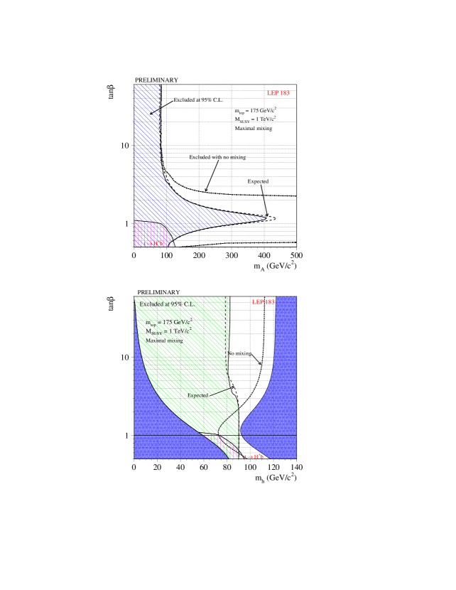
Figure 6: LEP200 limits for$M_{h}$ and $M_{A}$ as a function of $\tan\beta$, from Ref. 57.

Although the SUSY SM is rather predictive when it comes to the Higgs sector, beyond this sector the spectrum of SUSY partners and possible allowed interactions is quite model dependent. Most supersymmetric extensions of the SM considered are assumed to contain a discrete symmetry, $R$-parity, which is conserved. This assumption simplifies considerably the form of the possible interactions one has to consider. In fact, $R$-parity conservation provides an essentially unique way to generalize the SM since $R$, defined by

$$R=(-1)^{Q+L+2J}~{},$$ (122)

with $Q$ being the quark number, $L$ the lepton number and $J$ the spin, turns out simply to be +1 for all particles and -1 for all sparticles.

Obviously, $R$ parity conservation implies that SUSY particles enter in vertices always in pairs, and hence sparticles are always pair produced. This last fact implies, in turn, the stability of the lightest supersymmetric particle (LSP), even in the presence of supersymmetry breaking interactions. Although supersymmetry must be broken, since we do not observe multiplets of particles and sparticles of the same mass, SUSY breaking interactions are quite restrictive and do not end up by violating the stability of the LSP. Let me discuss the issue of SUSY breaking in a little more detail, since the manner in which one breaks supersymmetry is the principal source of model-dependence for the SUSY SM.

In general, $\!{}^{{\bf?}}$ one assumes that SUSY is spontaneously broken at some scale $\Lambda$ in some hidden sector of the theory. This sector is coupled to ordinary matter by some messenger states of mass $M$, with $M\gg\Lambda$, and all that obtains in the visible sector is a set of soft SUSY breaking terms—terms of dimension $d<4$ in the Lagrangian of the theory. Ordinary matter contains supersymmetric states with masses $\tilde{m}\sim$ TeV, with $\tilde{m}$ given generically by

$$\tilde{m}\sim\frac{\Lambda^{2}}{M}~{}.$$ (123)

Within this general framework, two distinct scenarios have been suggested which differ in what one assumes are the messengers that connect the hidden SUSY breaking sector with the visible sector. In supergravity models $\!{}^{{\bf?}}$ (SUGRA), the messengers are gravitational interactions, so that $M\sim M_{\rm Planck}$. Then, because of Eq. (120) and the demand that $\tilde{m}\sim$ TeV, the scale of SUSY breaking in the hidden sector is of order $\Lambda\sim 10^{11}$ GeV. In contrast, in models where the messengers are gauge interactions  $\!{}^{{\bf?}}$ (Gauge Mediated Models) with $M\sim 10^{6}$ GeV, then the scale of spontaneous breaking of supersymmetry is around $\Lambda\sim 10^{3}$ TeV.

In both cases one assumes that the supersymmetry is a local symmetry, gauged by gravity. $\!{}^{{\bf?}}$ Then the massless fermion which originates from spontaneous SUSY breaking, the goldstino, is absorbed and serves to give mass to the spin-3/2 gravitino—the SUSY partner of the graviton. This mass is of order

$$m_{3/2}\sim\frac{\Lambda^{2}}{M_{\rm P}}~{}.$$ (124)

Obviously, in SUGRA models the gravitino has a mass of the same order as all the other SUSY partners ($\tilde{m}\sim$ TeV). However, in SUGRA models, in general, one does not assume that the gravitino is the LSP. However, in Gauge Mediated Models, since $\Lambda\ll 10^{11}$ GeV, the gravitino is definitely the LSP.

Besides the above difference, the other principal difference between SUGRA and Gauge Mediated Models of supersymmetry breaking is the assumed form of the soft breaking terms. In SUGRA models, to avoid FCNC problems, one needs to assume that the soft breaking terms are universal. This assumption is unnecessary in Gauge Mediated Models, where in fact one can explicitly compute the form of the soft breaking terms and show that they do not lead to FCNC. Let me discuss this a little further.

The basic point is the following. As I alluded to earlier [cf. Eq. (107)], as a result of supersymmetry breaking one ends up, in general, with nondiagonal mass terms for the scalar fields $\phi_{i}$:

$${\cal{L}}_{\stackrel{{\scriptstyle\rm soft}}{{\rm mass}}}=-\sum_{ij}\mu^{2}_{oij}\phi_{i}^{\dagger}\phi_{j}~{}.$$ (125)

These terms, which connect states of the same charge, can lead to large FCNC through effective mass diagonal couplings of gluinos to squarks and quarks. The scalar mass insertion (122) gives rise to a $\tilde{g}d_{L}\tilde{s}_{L}$ vertex. Such a vertex can generate a very large $K^{o}-\bar{K}^{o}$ mixing term, through a gluino-squark box graph. With SUSY masses in the TeV range, this would be a total disaster. Hence, effectively, only diagonal soft mass terms can be countenanced. In the SUGRA models, this circumstance forces one to consider only universal soft breaking terms, with

$$\mu^{2}_{oij}=\mu^{2}_{o}\delta_{ij}~{}.$$ (126)

In the case of Gauge Mediated Models, this flavor blindness arises more naturally since SUSY breaking is the result of gauge interactions which are flavor diagonal. As a result, the soft mass terms can only couple diagonally and the soft masses will be proportional to the gauge couplings squared. One can show that the soft mass for the $i^{\rm th}$ scalar field is given by $\!{}^{{\bf?}}$

$$\mu_{i}^{2}=\sum^{3}_{a=1}\frac{\alpha_{a}^{2}}{(4\pi)^{2}}C_{i}\frac{\Lambda^{4}}{M^{2}}~{},$$ (127)

where $C_{i}$ is the appropriate Casimir factor for the scalar field in question. It follows from this equation that in Gauge Mediated Models, in general, squarks are heavier than sleptons since the latter do not have strong interactions. In SUGRA models both squarks and sleptons are assumed to have the same mass at large scales $(\mu\stackrel{{\scriptstyle>}}{{{}_{\scriptstyle\sim}}}\Lambda)$. However, as a result of the evolution of couplings these universal masses can become quite different at scales of order 100 GeV. Thus SUGRA models at low scales turn out to be not so dissimilar in their spectrum to Gauge Mediated Models.

This point is particularly germane for gauginos, where the differences between SUGRA and Gauge Mediated Models are quite small. For Gauge Mediated Models, the analogous equation to Eq. (124) for gaugino masses is only quadratically dependent on the gauge couplings $\!{}^{{\bf?}}$

$$m_{a}=\frac{\alpha_{a}}{4\pi}\frac{\Lambda^{2}}{M}~{}.$$ (128)

Hence the ratio of the $SU(3)$, $SU(2)$ and $U(1)$ gaugino masses scale with the $\alpha_{i}$

$$m_{1}:m_{2}:m_{3}=\alpha_{1}:\alpha_{2}:\alpha_{3}~{}.$$ (129)

In SUGRA models, although at high scales one assumes a universal gaugino mass $m_{1/2}$, the masses of the individual gauginos evolve in the same way as the squared gauge coupling constants

$$\frac{dm_{i}}{d\ln\mu^{2}}=-\frac{1}{16\pi^{2}}b_{i}m_{i}~{}.$$ (130)

Whence, at low scales, Eq. (126) holds again. As a result, the most important difference between these two SUSY breaking scenarios is that in Gauge Mediated Models the gravitino is the LSP, while in SUGRA models, the LSP is, in general, thought to be a neutralino—a spin-1/2 partner to the neutral gauge and Higgs bosons.

In Gauge Mediated Models, because the gravitino is the LSP, an important role for phenomenology is played by the “next lightest” SUSY state—the NLSP. In general, the NLSP in these models is either a slepton or a neutralino $\!{}^{{\bf?}}$ and, because it is not the lightest, this NLSP is unstable. The decay

$${\rm NLSP}\to\mbox{ordinary state + gravitino}$$ (131)

has a lifetime which scales as

$$\tau_{\rm NLSP}\to\frac{\Lambda^{4}}{M^{5}_{\rm NLSP}}~{}.$$ (132)

Depending on whether the NLSP decays occur within, or outside, the detector, the phenomenology of the Gauge Mediated Models will be similar, or rather different, to that of SUGRA models. This is because the gravitino acts essentially as missing energy, which is the signal associated with the SUGRA LSP.

I will not explicitly discuss here what are the expected signals for either the SUGRA or the Gauge Mediated scenarios, since the expected phenomenology is both involved and quite dependent on the actual spectrum of supersymmetric states assumed. $\!{}^{{\bf?}}$ I note here only that the present Tevatron and LEP 200 lower bounds on SUSY-states, although somewhat model dependent, are in the neighborhood of 100 GeV. More precisely, the weakest bounds are for the neutralinos $(M_{\chi^{o}}\stackrel{{\scriptstyle>}}{{{}_{\scriptstyle\sim}}}30$ GeV), followed by charginos $(M_{\chi^{\pm}}\stackrel{{\scriptstyle>}}{{{}_{\scriptstyle\sim}}}70$ GeV), sleptons $(M_{\tilde{\ell}}\stackrel{{\scriptstyle>}}{{{}_{\scriptstyle\sim}}}90$ GeV) and squarks and gluinos $(m_{\tilde{q}},m_{\tilde{g}}\stackrel{{\scriptstyle>}}{{{}_{\scriptstyle\sim}}}200$ GeV). $\!{}^{{\bf?}}$

Before closing this Section, I would like to make two final points concerning the SUSY alternative. These are

i) Not only does supersymmetry allow for a stable hierarchy between the Planck mass and the Fermi scale, but supersymmetry breaking itself can help trigger the $SU(1)\times U(1)\to U(1)_{\rm em}$ breaking. The Higgs mass matrix ${\cal{M}}^{2}$ can start with ${\rm det}~{}{\cal{M}}^{2}>0$ at high scales but can evolve to ${\rm det}~{}{\cal{M}}^{2}<0$ at the Fermi scale. Indeed $m_{2}^{2}$, the mass term associated with the $H_{u}$ Higgs, is strongly affected by the large top Yukawa coupling and can change sign as one evolves to low $q^{2}$. This radiative breaking of $SU(2)\times U(1)$, triggered by SUSY breaking, $\!{}^{{\bf?}}$ is a very attractive feature of the SUSY SM. For it to produce the Fermi scale, however, one must inject already at very high scales a SUSY breaking mass parameter also of order $v_{F}$. Why this should be so remains a mystery.

ii) In SUGRA models the neutralino LSP, which is a linear combination of all the neutral weak gaugino and Higgsino fields

$$\tilde{\chi}=\alpha_{\gamma}\tilde{\gamma}+\alpha_{Z}\tilde{Z}+\alpha_{u}\tilde{H}_{u}+\alpha_{d}\tilde{H}_{d}$$ (133)

is an excellent candidate for cold dark matter. $\!{}^{{\bf?}}$ In the Gauge Mediated case, the gravitino could provide a warm dark matter candidate, $\!{}^{{\bf?}}$ provided that

$$m_{3/2}\sim\frac{\Lambda^{2}}{M_{\rm P}}\sim{\rm KeV}~{},$$ (134)

which requires $\Lambda\sim 10^{3}$ TeV. The presence of possible candidates for the dark matter in the Universe, is another quite remarkable feature of low energy SUSY models and speaks in favor of the SUSY alternative.

6 Are there Extra Dimensions of Size Greater than a (TeV)^-1?

To conclude these lectures, I want to make some remarks on the phenomenological consequences of imagining that the Fermi scale is associated with the Planck scale of $(d+4)$-dimensional gravity. That is

$$v_{F}\sim(M_{\rm P})_{d+4}\equiv M~{}.$$ (135)

The extra $d$-dimensions in this theory are assumed to be compact and of size $R$. By comparing the Newtonian forces in $(d+4)$-dimensions with that in four dimensions, one can interrelate $M$ and the usual Planck mass $M_{\rm P}=G_{N}^{-1/2}\simeq 10^{19}$ GeV. $\!{}^{{\bf?}}$ One has

$$F_{4}=\frac{1}{M_{\rm P}^{2}}\frac{m_{1}m_{2}}{r^{2}}~{};~{}~{}~{}F_{4+d}=\frac{1}{(M)^{2+d}}\frac{m_{1}m_{2}}{r^{d+2}}~{}.$$ (136)

Then, using Gauss’ law, it follows that $\!{}^{{\bf?}}$

$$M_{\rm P}=M(MR)^{d/2}~{}.$$ (137)

Obviously, demanding that $M$ be of the order of the Fermi scale $v_{F}$, fixes the size $R$ of the compact dimensions as a function of the number of these extra dimensions $d$. One finds that for $d=2$, $R\sim 10^{-1}$ cm, while for $d=6$, $R\simeq 10^{-13}$ cm. For distances $r$ below the size $R$ of the compact dimensions one will begin to register the fact that gravitational forces do not follow the familiar $r^{-2}$ law. Thus the first test that this idea is not nonsensical is to look for possible modifications of the usual Newtonian potential at short distances. For $r\sim R$, the potential will feel Yukawa-like correctione of strength $2d$: $\!{}^{{\bf?}}$

$$V(r)=-\frac{G_{N}m_{1}m_{2}}{r}\left\{1+2de^{-r/R}+\ldots\right\}~{}.$$ (138)

There have been a variety of tests of the Newtonian potential at (relatively) short distances. For $r>100\mu$, the most stringent limits for deviation from the Newtonian expectations $\!{}^{{\bf?}}$ allow $R\sim 10^{-1}$ cm for strengths $\alpha\equiv 2d$ of $O(1)$. Below $100\mu$, the best bounds on non-Newtonian forces come from Casimir experiments but, as shown in Fig. 7, these experiments only put some constraints on modifications which have a strength $\alpha$ much below unity. This figure also shows the limits which might be achievable in a proposed experiment employing 1 KHz mechanical oscillators as test masses. This experiment $\!{}^{{\bf?}}$ should be able to push $\alpha$ to $\alpha\sim 10^{-1}$ for compact dimensions $R\sim 10^{-1}$ cm. Thus it could directly test for deviations from Newtonian gravity to a level where an effect might be seen.

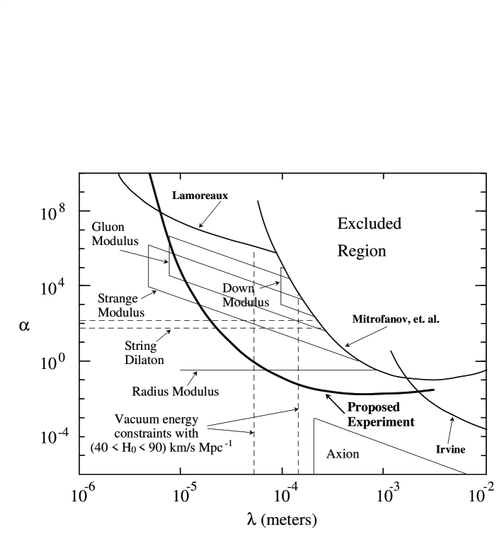
Figure 7: Experimental status of gravitational strength forces at short distances, from Ref. 67.

At high energy, the presence of extra compact dimensions of finite size $R$ can be detected because these theories allow abundant graviton production to occur. Obviously, to see any effects one needs experiments at energies $(\sqrt{s})_{\rm parton}\sim M\sim v_{F}$– energies which will be attainable at the LHC. The presence of compact dimensions of size $R$ allows gravitons to get produced, at energies of order $(\sqrt{s})_{\rm parton}\sim M$, with a probability proportional to $M^{-2}$ not $M_{\rm P}^{-2}$. However, the graviton production is rather soft, with the softness being greatest the larger the number of compact dimensions $d$ is.

This can be understood qualitatively as follows. In the theories under discussion, the SM fields exist essentially on a 4-dimensional hypersurface, with gravity acting both on this hypersurface, as well as on a set of compact dimensions of size $R$. From the point of view of the 4-dimensional theory, a graviton with its momentum $p^{\alpha}$ acting in the compact dimensions is equivalent to having a particle of mass

$$m_{\rm eff}\sim\frac{i}{R}~{},$$ (139)

where $i$ is an integer associated with the level of excitation. It follows that, for given total energy $E$, one can access many states in the compact dimensions. Using (136), the spacing among these states is of order $\Delta E\sim R^{-1}$. Thus, for processes of total energy, $E$, the total number of states probed in the compact dimensions is

$$N\sim\left(\frac{E}{\Delta E}\right)^{d}\sim(RE)^{d}~{}.$$ (140)

The probability of gravitational production at $(\sqrt{s})_{\rm parton}=E$ is inversely proportional to the Planck mass $M_{\rm P}$, but directly proportional to the number of states $N$ excited in the compact dimensions. If $N$ is large, which will occur for $E\gg R^{-1}$, then, effectively, the probability of producing gravitational radiation is much greater than the classical expectations. Indeed, as alluded to above, this probability scales like $M^{-2}$ not $M_{\rm P}^{-2}$. One has

$${\rm Probability}\sim\frac{1}{M_{\rm P}^{2}}N\sim\frac{(ER)^{d}}{M_{\rm P}^{2}}=\frac{(ER)^{d}}{M^{2+d}R^{d}}=\frac{1}{M^{2}}\left(\frac{s}{M^{2}}\right)^{d/2}~{}.$$ (141)

Note, however, that even though the probability indeed scales like $M^{-2}$ there is an additional soft infrared multiplying factor of $(s/M^{2})^{d/2}$. Therefore, one learns that strong graviton production comes on slowly for $s<M^{2}$. Thus the importance of these effects for the LHC, even if these theories were to be true, is crucially dependent on the value of $M$.

Mirabelli, Perelstein and Peskin, $\!{}^{{\bf?}}$ as well as others, $\!{}^{{\bf?}}$ have studied graviton production at LEP and Tevatron energies to try to obtain bounds on $M$ from present day data. These authors have looked for the processes $e^{+}e^{-}\to\gamma G$ and $p\bar{p}\to{\rm jet}~{}G$, with the graviton experimentally being manifested as missing energy. Analyses of the LEP data for the process $e^{+}e^{-}\to\gamma\nu\bar{\nu}$ and of the CDF/DO bounds for monojet production yield the bounds:

$$M\stackrel{{\scriptstyle>}}{{{}_{\scriptstyle\sim}}}600{\rm GeV}~{}~{}(d=6);~{}~{}~{}~{}M\stackrel{{\scriptstyle>}}{{{}_{\scriptstyle\sim}}}750{\rm GeV}~{}~{}(d=2).$$ (142)

Obviously the LHC will be sensitive to much greater values of $M$. However, at least for $d=2$, astrophysics already puts a strong constraint on $M$. Basically, if $M$ is too low graviton emission will cool off supernovas too quickly. The fact that SN 1987a does not show any anomalous cooling then allows one to set a bound of $M\stackrel{{\scriptstyle>}}{{{}_{\scriptstyle\sim}}}30$ TeV, for $d=2$. $\!{}^{{\bf?}}$

7 Concluding Remarks

In these lectures I have discussed the theoretical arguments for believing that there is physics beyond the electroweak theory, related to the origin and magnitude of the Fermi scale $v_{F}$. Each of the suggestions for new physics which I examined: dynamical symmetry breaking, supersymmetry and extra compact dimensions, had its own characteristic signals and its own set of theoretical puzzles to resolve. A priori, it is clearly not possible to select among these alternatives purely theoretically. However, from the few meager experimental hints for physics beyond the SM that we have today, supersymmetry does appear to be favored. What is exciting is that we should know quite soon which of these alternatives, if any, are correct. If one is lucky, the answer may come perhaps already from experiments at LEP200 or the Tevatron. However, the origin of the Fermi scale should certainly become clear once the LHC starts running.

References

References

- [1] For an introduction to the Standard Model see, for example, my lectures, and those of others, at TASI 90, Testing the Standard Model, Proceedings of the 1990 Theoretical Advanced Study Institute in Elementary Particle Physics, eds. M. Cvetic and P. Langacker (World Scientific, Singapore 1991). A subset of the original references includes: S. L. Glashow, Nucl. Phys. B22 (1961) 579; S. Weinberg, Phys. Rev. Lett. 19 (1967) 1264; A. Salam, in Elementary Particle Theory, ed. N. Svartholm (Amquist and Wiksels, Stockholm 1969); H. Fritzsch, M. Gell-Mann and H. Leutwyler, Phys. Lett. 47 (1973) 365; H. D. Politzer, Phys. Rev. Lett. 30 (1973) 1346: D. Gross and F. Wilczek, Phys. Rev. Lett. 30 (1973) 1343; S. Weinberg, Phys. Rev. Lett. 31 (1973) 494.
- [2] M. W. Grünewald, in the Proceedings of the 29th Conference on High Energy Physics, ICHEP98, Vancouver, Canada, July 1998, eds. A. Astbury, D. Axen and J. Robinson (World Scientific, Singapore 1999) p569.
- [3] SuperKamiokande Collaboration, Y Fukuda et al., Phys. Rev. Lett. 81 (1998) 1562.
- [4] For a discussion see, for example, R. D. Peccei in Concepts and Trends in Particle Physics, eds. H. Latal and H. Mutter, in Proceedings of the XXV Int. Universität Wochen für Kernphysik, Schladming, Austria, 1986 (Springer-Verlag, Berlin 1987).
- [5] For a discussion see, for example, R. D. Peccei, hep-ph/9906509, to be published in the Proceedings of the VIII Escuela Mexicana de Particulas y Campos, Oaxaca, Mexico, 1998.
- [6] For a discussion see, for example, A.L. Fetter and J. D. Walecka, Quantum Theory of Many Particle Systems (McGraw Hill Book Company, New York 1971).
- [7] M. Aizenman, Comm. Math. Phys. 86 (1982) 1; J. Frölich, Nucl. Phys. B200 [FS4] (1982) 281.
- [8] L. Landau in Niels Bohr and the Development of Physics, ed. W. Pauli (McGraw Hill, New York 1955).
- [9] G. ’t Hooft, in Recent Developments in Gauge Theories, Proceedings of the Nato Advanced Study Institute, Cargese, France, 1979, eds G. ’t Hooft et al. (Plenum Press, New York 1980)
- [10] M. Luescher and P. Weisz, Nucl. Phys. B290 (1987) 25: B295 (1988) 65: B318 (1989) 705; J. Kuti, L. Lin and Y. Shen, Phys. Rev. Lett. 61 (1988) 678; A. Hasenfratz et al., Phys. Lett. 199B (1987) 531; Nucl. Phys. B317 (1989) 81; G. Bhanot et al., Nucl. Phys. B343 (1990) 467; B353 (1991) 551.
- [11] For an introduction see, for example, J. Wess and J. Bagger, Supersymmetry and Supergravity ( Princeton University Press, Princeton 1992) Edition.
- [12] N. Arkani-Hamed, S. Dimopoulos and G. Dvali, Phys. Lett. B429 (1998) 263; Phys. Rev. D59 (1999) 086004; I. Antoniadis, S. Dimopoulos and G. Dvali, Nucl. Phys. B516 (1998) 70; I. Antoniadis, N. Arkani-Hamed, S. Dimopoulos and G. Dvali, Phys. Lett. B436 (1998) 257.
- [13] I. Antoniadis, Phys. Lett. B246 (1990) 377; Proceedings of the PASCOS-91 Symposium, Boston, Mass. (World Scientific, Singapore 1991); see also, J. Lykken, Phys. Rev. D54 (1996) 3693.
- [14] The data from the Tevatron is summarized by E. Barberis and W. -M. Yao, in the Proceedings of the 29th Conference on High Energy Physics, ICHEP98, Vancouver, Canada, July 1998, eds. A. Astbury, D. Axen and J. Robinson (World Scientific, Singapore 1999) p1098 and p1093.
- [15] The fits to the SM of precision electroweak data are summarized by D. Karlen, in the Proceedings of the 29th Conference on High Energy Physics, ICHEP98, Vancouver, Canada, July 1998, eds. A. Astbury, D. Axen and J. Robinson (World Scientific, Singapore 1999) p47; see, also, Ref. 31.
- [16] The data from LEP200 is summarized by P. A. McNamara, in the Proceedings of the 29th Conference on High Energy Physics, ICHEP98, Vancouver, Canada, July 1998, eds. A. Astbury, D. Axen and J. Robinson (World Scientific, Singapore 1999) p1303.
- [17] M. Veltman, Acta Phys. Pol. B8 (1977) 475. The O() corrections to have been calculated by J. Van der Bij and M. Veltman, Nucl. Phys. B231 (1984) 205 and are proportional to .
- [18] M. E. Peskin and T. Takeuchi, Phys. Rev. Lett. 65 (1990) 964; Phys. Rev. D46 (1992) 381; B. Holdom and J. Terning, Phys. Lett.B247 (1990) 88; D. C. Kennedy and P. Langacker, Phys. Rev. Lett. 65 (1990) 2967; G. Altarelli and R. Barbieri, Phys. Lett. B253 (1990) 161; G. Altarelli, R. Barbieri and S. Jadach, Nucl. Phys. B369 (1992) 3; G. Altarelli, R. Barbieri and F. Caravaglios, Nucl. Phys. B405 (1993) 3; Phys. Lett. B349 (1995) 145.
- [19] M. E. Peskin and T. Takeuchi, Phys. Rev. D46 (1992) 381.
- [20] G. Altarelli, R. Barbieri and F. Caravaglios, Int. J. Mod. Phys. A13 (1998) 1031.
- [21] H. Georgi, H. R. Quinn and S. Weinberg, Phys. Rev. Lett. 33 (1974) 451.
- [22] R. Slansky, Phys. Reports 79C (1981) 1.
- [23] See, for example, U. Amaldi, W. de Boer and H. Fürstenau, Phys. Lett. B260 (1991) 447.
- [24] See, for example, M. Olechowski and S. Pokorski, Phys. Lett. B257, 388 (1991).
- [25] See, for example, B. Schrempp and M. Wimmer, Progr. in Part. and Nucl. Phys. 37 (1996) 1.
- [26] G. Altarelli and G. Isidori, Phys. Lett. B337 (1994) 141.
- [27] M. Lindner, Z. Phys. C31 (1986) 295.
- [28] B. Pendelton and G. G. Ross, Phys. Lett. B98 (1981) 291; C. T. Hill, Phys. Rev. D24 (1981) 691.
- [29] For a recent discussion see, for example, J. N. Bahcall, P. I. Krastev and A. Yu. Smirnov, Phys. Rev. D58 (1998) 096016.
- [30] T. Yanagida, in Proceedings of the Workshop on the Unified Theories and Baryon Number in the Universe, Tsukuba, Japan 1979, eds. O. Sawada and A. Sugamoto, KEK Report No. 79-18; M. Gell-Mann, P. Ramond and R. Slansky, in Supergravity, Proceedings of the Workshop at Stony Brook, NY, 1979, eds. P. van Nieuwenhuizen and D. Freedman (North-Holland, Amsterdam 1979).
- [31] See, for example, the compilation of the latest electroweak data from LEP and the SLC in the report of the LEP Electroweak Working Group, CERN-EP/99-15, February 1999.
- [32] See, for example, S. Weinberg, in Proceedings of the XXIII International Conference on High Energy Physics, Berkeley, California 1986, ed. S. C. Loken (World Scientific, Singapore 1987).
- [33] L. Susskind, Phys. Rev. D20, 2619 (1979); S. Weinberg, Phys. Rev. D13, 974 (1976).
- [34] See, for example, R. D. Peccei, in Broken Symmetries, eds. L. Mathelitsch and W. Plessas, Lecture Notes in Physics 521 (Springer Verlag, Berlin 1999).
- [35] See, for example, J. F. Donoghue, E. Golowich and B. R. Holstein, Dynamics of the Standard Model (Cambridge University Press, Cambridge, UK 1992).
- [36] S. Dimopoulos and L. Susskind, Nucl. Phys. B155 (1979) 237; E. Eichten and K. Lane, Phys. Lett. B90 (1980) 125.
- [37] S. Dimopoulos and J. Ellis, Nucl. Phys. B182 (1981) 505.
- [38] See, for example, E. Fahri and L. Susskind, Phys. Rept. 74C (1981) 277; see, also, Ref. 38
- [39] For an extensive review, see R. S. Chivukula, hep-ph/9803219, lectures presented at 1997 Les Houches Summer School, Les Houches, France.
- [40] B. Holdom, Phys. Rev. D24 (1981) 1441; K. Yamawaki, M. Bando, and K. Matsumoto, Phys. Rev. Lett. 56 (1986) 1335; T. Akiba and T. Yanagida, Phys. Lett. 169B (1986) 432; T. Appelquist, D. Karabali and L. Wijewardhana, Phys. Rev. Lett. 57 (1986) 982.
- [41] R. Sundrum and S. D. H. Hsu, Nucl. Phys. B391 (1993) 127.
- [42] H. Pagels, Phys. Rept. 16C (1975) 219.
- [43] K. Lane, Phys. Rev. D10 (1974) 2605; H. D. Politzer, Nucl. Phys. B117 (1976) 397.
- [44] See, for example, B. Holdom, Phys. Lett. B246 (1990) 169 ; see, also, B. Holdom in Dynamical Symmetry Breaking, ed. K. Yamawaki (World Scientific, Singapore 1992); R. Sundrum, Nucl. Phys. B395 (1993) 60.
- [45] R. S. Chivukula, S. B. Selipsky and E. H. Simmons, Phys. Rev. Lett. 69 (1992) 575.
- [46] C. T. Hill, Phys. Lett. B345 (1995) 483; E. Eichten and K. Lane, Phys. Lett. B352 (1995) 382; K. Lane, Phys. Rev. D54 (1996) 2204.
- [47] Y. Nambu, in Proceedings of the 1988 International Workshop on New Trends in Strong Coupling Gauge Theories, Nagoya, Japan, eds. M. Bando, T. Muta and K. Yamawaki; V. A. Miransky, M. Tanabashi and K. Yamawaki, Mod. Phys. Lett. A4 (1989) 1043; W. A. Marciano, Phys. Rev. Lett. 62 (1989) 2793; W. A. Bardeen, C.T. Hill and M. Lindner, Phys. Rev. D41 (1990) 1647.
- [48] E. Eichten, K. Lane and J. Womersley, Phys. Lett. B405 (1997) 305.
- [49] For reviews see, for example, H. P. Nilles, Phys. Rept. 110C (1984) 1; H. E. Haber and G. L. Kane, Phys. Rept. 117C (1985) 75.
- [50] C. Bouchiat, J. Iliopoulos and Ph. Meyer, Phys. Lett. B38 (1972) 519; D. J. Gross and R. Jackiw, Phys. Rev. D6 (1972) 477.
- [51] E. Cremmer, S. Ferrara, L. Girardello and A. Van Proyen, Nucl. Phys. B212 (1983) 506; L. Girardello and M. Grisaru, Nucl. Phys. B194 (1984) 65.
- [52] J. F Gunion, H. E. Haber, G. Kane and S. Dawson, The Higgs Hunter’s Guide ( Addison-Wesley Publishing Company, Reading, Mass 1990).
- [53] H. E. Haber and R. Hempfling, Phys. Rev. Lett. 66 (1991) 1815; Y. Okada, M. Yamaguchi and T. Yanagida, Prog. Theo. Phys 85 (1991) 1; J. Ellis, G. Ridolfi and F. Zwirner, Phys. Lett. B257 (1991) 83; B262 (1991) 477.
- [54] S. Heinemeyer, W. Hollik and G. Weiglein, Phys. Rev. D48 (1998) 091701; Phys. Lett. B440 (1998) 296; B455 (1999) 179; see, also, R. Hempfling and A. H. Hoang, Phys. Lett. 331 (1994) 99; R. -J. Zhang, Phys. Lett. B447 (1999) 89.
- [55] For a review see, for example, H. E. Haber, hep-ph/9901365, to appear in the Proceedings of the 4th International Symposium on Radiative Corrections (RADCOR 98), Barcelona, Spain, 1998.
- [56] R. -J. Zhang, Phys. Lett. B447 (1999) 89.
- [57] The data from LEP is summarized by K. Desch, in the Proceedings of the 29th Conference on High Energy Physics, ICHEP98, Vancouver, Canada, July 1998, eds. A. Astbury, D. Axen and J. Robinson (World Scientific, Singapore 1999) p1309.
- [58] For a discussion see, for example, M. E. Peskin, hep-ph/9705479, lectures presented at the 1996 European School of High Energy Physics, Carry-le Rouet, France.
- [59] For reviews see, for example, P. Nath, R. Arnowitt and A. H. Chamseddine, Aplied N=1 Supergravity (World Scientific, Singapore 1984); R. Arnowitt and P. Nath, Proceedings of the VII J. A. Swieca Summer School, ed. E. Eboli (World Scientific, Singapore 1994).
- [60] M. Dine and A. E. Nelson, Phys. Rev. D48 (1993) 1277; M. Dine, A. E. Nelson and Y. Shirman, Phys. Rev. D51 (1995) 1362; M. Dine, A. E. Nelson, Y. Nir and Y. Shirman, Phys. Rev. D53 (1996) 2658; for a review, see G. F. Giudice and R. Rattazzi, hep-ph/9801271.
- [61] S. Ferrara, D. Z. Freedman and P. van Nieuwenhuizen, Phys. Rev. D13 (1976) 3214.
- [62] For a review of SUSY searches, see D. Treille, in the Proceedings of the 29th Conference on High Energy Physics, ICHEP98, Vancouver, Canada, July 1998, eds. A. Astbury, D. Axen and J. Robinson (World Scientific, Singapore 1999) p87.
- [63] L. Ibaez and G. G. Ross, Phys. Lett. B110 (1982) 215: L. Alvarez-Gaume, M. Clauson and M. B. Wise, Nucl. Phys. B207 (1982) 96.
- [64] See, for example, A. Bottino, F. Donato, G. Mignola, S. Scopel, P. Belli, and A. Incicchiti, Phys. Lett. B402 (1997) 103; see also A. Bottino, astro-ph/9611137, invited talk at the International Workshop on the Identification of Dark Matter, Sheffield, UK, 1996.
- [65] See, for example, S. Borgani, A. Masiero, and M. Yamaguchi, Phys. Lett. 356B (1996) 189.
- [66] E. A. Mirabelli, M. Perelstein and M. E. Peskin, Phys. Rev. Lett. 82 (1999) 2236.
- [67] For a recent review, see J. C. Long, H. W. Chan and J. C. Price Nucl. Phys. B539 (1999) 23.
- [68] T. Han, J. D. Lykken and R.-J. Zhang, Phys. Rev. D59 (1999) 105006; G. F. Giudice, R. Rattazzi and J. D. Wells, Nucl. Phys. B544 (1999) 3.
- [69] N. Arkani-Hamed, S. Dimopoulos and G. Dvali, Phys. Rev. D59 (1999) 086004.