SLAC-PUB-8218 September 1999

Testing the Nature of Kaluza-Klein Excitations at Future Lepton Colliders

Thomas G. Rizzo

Stanford Linear Accelerator Center

Stanford University

Stanford CA 94309, USA

With one extra dimension, current high precision electroweak data constrain the masses of the first Kaluza-Klein excitations of the Standard Model gauge fields to lie above $\simeq 4$ TeV. States with masses not much larger than this should be observable at the LHC. However, even for first excitation masses close to this lower bound, the second set of excitations will be too heavy to be produced thus eliminating the possibility of realizing the cleanest signature for KK scenarios. Previous studies of heavy $Z^{\prime}$ and $W^{\prime}$ production in this mass range at the LHC have demonstrated that very little information can be obtained about their couplings to the conventional fermions given the limited available statistics and imply that the LHC cannot distinguish an ordinary $Z^{\prime}$ from the degenerate pair of the first KK excitations of the $\gamma$ and $Z$. In this paper we discuss the capability of lepton colliders with center of mass energies significantly below the excitation mass to resolve this ambiguity. In addition, we examine how direct measurements obtained on and near the top of the first excitation peak at lepton colliders can confirm these results. For more than one extra dimension we demonstrate that it is likely that the first KK excitation is too massive to be produced at the LHC.

1 Introduction

If Kaluza-Klein excitations of the Standard Model(SM) gauge fields exist then analyses of precision electroweak data indicate that the masses of the first excitation of the $W$, $Z$, $\gamma$ and $g$ must be greater than $\simeq 4$ TeV in the case of one extra dimension. For such heavy masses the second set of excitations will lie beyond the reach of the LHC even at several times design luminosity. In addition, the limited statistics at such large invariant masses will ($i$) most likely render the gluon excitation invisible due to both its large width to mass ratio as well as detector jet energy smearing and ($ii$) will not allow the photon and Z resonances to be resolved even if they are not exactly degenerate. Thus the LHC will see what appears to be a degenerate $Z^{\prime}$ and $W^{\prime}$, something that occurs in many more ordinary extended electroweak gauge models. Based upon past studies of new gauge boson coupling determinations at hadron colliders we know that with the available statistics the LHC will not be able to identify these resonances as KK excitations. How can we resolve this issue? As we will show below, a lepton collider, even one operating reasonably far below the apparent $Z^{\prime}$ resonance will most likely provide evidence compelling enough to resolve this ambiguity. Furthermore, we will demonstrate that a higher energy lepton collider, sitting on this resonance peak, will very easily distinguish the two possibilities not via an analysis of the line shape but through several factorization tests among electroweak observables. The extension to the case of more than one extra dimension is also discussed.

This paper is organized as follows: Section 2 contains a pedagogical theory background for the definition of the problem and the analysis that follows. The details of the problem outlined above are discussed in Section 3. In Section 4 we discuss how a linear collider operating at energies well below the mass of the first KK excitations, presumed discovered at the LHC, will yield strong evidence about its fundamental nature while in Section 5 we discuss what additional information can be learned by sitting on the KK resonance at a future lepton collider. A summary and further discussion is given in Section 6.

2 Background

String/M-theory tells us that we live in a world with at least six extra dimensions. It is perhaps likely that the size of these dimensions are of order the inverse Planck scale, $\sim 1/M_{pl}$, and may remain forever hidden from direct experimental confirmation. However, in the past two years the possibility has re-emerged[1] that at least some of these extra dimensions may be much larger and not far away from the electroweak scale, $\sim 1/$TeV, that is now being probed at colliders. In one appealing scenario[2] due to Arkani-Hamed, Dimopoulos and Dvali(ADD), gravity is allowed to propagate in at least two ‘large’ extra dimensions while the fields of the SM are confined to D-branes of appropriate dimension transverse to these. (Here by ‘large’ we mean compactification radii $>>1/$TeV.) Such a structure allows for the Planck scale to be brought down from $10^{19}$ GeV to only a few TeV offering a new slant on the hierarchy problem. The specific size of these ‘large’ dimensions depend on how many we assume there to be; for $n$ extra ‘large’ dimensions the common compactification radius $R$ is order $\sim 10^{30/n-19}$ m. The rich phenomenology of this model has been examined in a very rapidly growing series of papers[3]. (We note in passing that the ADD scenario assumes that the metric tensor on the brane does not depend on the compactified co-ordinates, i.e., that it factorizes; this need not be necessary[4].) If $n<6$ there can also be some extra ‘small’ longitudinal dimensions wherein both the SM fields as well as gravity can live. (Here by ‘small’ we mean compactification radii $\sim 1/$TeV.) For example, we can imagine there being 4 ‘large’ extra dimensions in which only gravity propagates and 2 ‘small’ extra dimensions populated by both gravity as well as the SM gauge fields. The propagation of the SM fields into these ‘small’ dimensions can lead to a drastic lowering of the GUT scale[5] due to an almost power-like running of the couplings. There are many variations on this particular theme depending upon which and how many SM fields we allow to feel the extra dimensions. In what may be the most well motivated and attractive scheme, and the one we consider below, only the SM gauge fields (and the Higgs field) can propagate in the extra dimensions while the chiral fermions only experience the usual four dimensions and thus lie on a 3-brane, i.e., ‘the wall’. (We imagine that all of the SM gauge fields feel the same number of the extra dimensions in what follows.) It is now possible to imagine a viable scenario wherein the Planck, string, compactification and GUT scales are not too far above a few TeV.

In addition to probing weak scale gravity[3] another test of this scenario is to search for the Kaluza-Klein(KK) excitations of the SM gauge fields. In fact, the hallmark[1, 6] of these KK theories is the existence of regularly spaced resonances in the $\ell^{+}\ell^{-}$, $\ell^{\pm}\nu$ and $jj$ channels at hadron colliders, such as the Tevatron and LHC, which are degenerate, i.e., the first excitations, $\gamma^{(1)},Z^{(1)},W^{(1)}$ and $g^{(1)}$, have a common mass, in the limit that mixing with the corresponding SM zero modes is neglected. (In practice, even when mixing is present the fractional mass shifts are quite negligible for KK states above 1 TeV.) As we will see below, such recurrence structures are not always observable making the direct experimental case for KK scenarios less transparent. For one extra longitudinal dimension, compactification on $S^{1}/Z_{2}$ leads to equally spaced states with masses given by $M_{n}=n/R$ and with a non-degenerate level structure. Due to the normalization of the gauge field kinetic energies, the excitations in the KK tower naively couple to the SM fermions with a strength larger than that of the zero-modes by a universal factor of $\sqrt{2}$ assuming that the fermions are all localized at the same fixed point on the wall[7]. (More on this point below.) For the case of more than one extra dimension the situation is far more complex and depends upon the details of the compactifying manifold. Here we find that not only are the KK excitation spacings more intricate but many of the levels become degenerate and the strength of the coupling in comparison to the zero-modes becomes level dependent. For example, in the case of two additional dimensions with a $S^{1}/Z_{2}\times S^{1}/Z_{2}$ compactification, assuming both compactification radii are equal, the first five KK levels occur at masses of (in units of $1/R$) $1,\sqrt{2},2,\sqrt{5}$ and $\sqrt{8}$ with degeneracies of $2,1,2,2$ and 1 and with naive relative coupling strengths of $\sqrt{2},2,\sqrt{2},2$ and 2, respectively. Alternative compactifications yield other more intricate patterns as do extensions to the case of even more dimensions.

What do we know about the size of the compactification radii for these longitudinal dimensions, i.e., what bounds are there on the masses of the SM excitations? From direct searches for $Z^{\prime}$, $W^{\prime}$ and dijet bumps at the Tevatron[8], it is clear that the masses of the first tower states are in excess of $\sim 0.7-0.9$ TeV. Through cross section and asymmetry measurements at LEP II the anticipated reach for the first KK state through indirect means will be approximately 3 TeV by combining the results of all four experiments assuming adequate luminosity is achieved. However, by examining the influence of KK towers on electroweak measurements[9] we can place far tighter bounds on $1/R$, or equivalently, the first excitation masses provided we make a number of assumptions. First, as is usual in these types of analyses, it is assumed that the KK fields are the only source of new physics that perturb the SM predictions for electroweak quantities. Secondly, we must assume that the couplings of at least the first few recurrences to the SM fields are not vastly different than those given by the simple rescaling correction due to the normalization of the gauge field kinetic energies discussed above. The reason to worry about this particular assumption is clear by considering the limit wherein the effects of KK tower exchanges can be written as a set of contact interactions by integrating out the tower fields. Almost all of the current constraints on the masses of KK states arise from consideration of this contact interaction limit. In this case tower exchanges lead to new dimension-six operators whose coefficients can be shown to be proportional to a fixed dimensionless quantity, $V$, which can be symbolically written as[10]

$$V=(M_{w}R)^{2}\sum_{{\bf n}=1}^{\infty}{g_{\bf n}^{2}\over{g_{0}^{2}}}{1\over{{\bf n}\cdot{\bf n}}}\,,$$ (1)

where $g_{\bf n}$ is the coupling of the $n^{th}$ KK level labelled by the set of integers n. $M_{w}$, is the $W$ boson mass which we employ as a typical weak scale. (Here for simplicity of presentation we have assumed a $Z_{2}\times Z_{2}\times...$ compactification so that the first KK excitation(s) has a mass $1/R$.) Through an analysis of precision measurements the value of $V$ can be directly restricted thus leading to an apparent constraint on $R$ for any given number of extra dimensions and specified compactification scenario. However, this seemingly straightforward program runs into an immediate difficulty requiring a somewhat detailed digression. The resolution of this difficulty has influence upon where we anticipate the mass of the KK excitations to lie and, through possible modifications their couplings to the fermions of the SM, their production cross sections at colliders.

Using the naive scaling of the couplings the sum in the expression above only converges (to a value of $2\sum_{n=1}^{\infty}1/n^{2}=\pi^{2}/3\simeq 3.28987$ assuming all the fermions are properly localized) in the case of a single extra dimension. There are several ways to deal with this problem. The first and most often used[5] approach is to sum over a finite number of terms, i.e., only those states whose masses lie below the string scale, $M_{s}$, which now acts simply as a cut off. For example, in the case of one extra dimension, we cut off the sum at $n=n_{max}\simeq M_{s}R$ and for any fixed assumed value of $M_{s}R$ we will of course obtain a smaller value than given by the complete sum. If $n_{max}=5(10,20)$ we obtain for the partial sum 2.92722(3.09954,3.19233), which are all not far from the value above due to the rapid convergence of the series. While this procedure does not numerically reduce the sum in any serious manner in the one dimensional case it has a far greater influence in more than one dimension since this partial sum is finite. For example, in the case of $Z_{2}\times Z_{2}$ taking $n_{max}=5$, so that we include only the first 14 mass states in the tower, yields a value of 12.7826 for the partial sum. Note that this is appreciably larger than in the one dimensional case. Taking instead $n_{max}=10(20)$ yields the corresponding results of 17.0790(21.4083) which shows an approximate logarithmic growth with increasing $n_{max}$. Given a fixed upper bound on the value of $V$ this would imply that the lower bound on the mass of the first KK excitation would have to be at least a factor of 2 larger than in the one-dimensional case. Even though the cross section for the production of this state would be 4 times larger than in the one dimensional case due to the enhanced coupling it is clear that this state would be to massive to be produced at the LHC. While this approach regularizes the tower sum, this straightforward truncation technique appears to be somewhat arbitrary and conceptually inadequate.

A second possibility is that the KK couplings to four dimensional fields have an additional level dependence, above and beyond that due to the appropriate kinetic energy normalization factor, that exponentially damps the contributions from higher terms in the sum[11]. Such a suppression has been suggested on several grounds including the high energy behaviour of string scattering amplitudes and also through considerations of the flexibility of the wall[11]. In the later case, for a rather rigid wall, the still infinite sum is now of the form

$$V=(M_{w}R)^{2}\sum_{{\bf n}=1}^{\infty}{g_{\bf n}^{2}\over{g_{0}^{2}}}{1\over{{\bf n}\cdot{\bf n}}}e^{-{\bf n}\cdot{\bf n}/n_{max}^{2}}\,,$$ (2)

where $n_{max}$ is as given above. For any given value of $n_{max}$ the sum is finite and, if $n_{max}$ is not too small the couplings of the first KK excitations hardly differ from their naive values. We note that for the case of one extra dimension taking $n_{max}=5(10,20)$ yields the sum 2.62089(2.94538, 3.11512), again not far from actual naive sum but somewhat smaller than in the simpler truncation of the summation approach. In addition, by absorbing the exponential into the definition of their strengths, the corresponding couplings of the first excitation relative to the zero mode is given by $g_{1}^{2}/2g_{0}^{2}=0.9608(0.9901,0.9975)$, respectively. Here we see that there is very little suppression in the strength of the couplings in comparison to the naive value obtained through from the gauge field kinetic terms. (We note that if we assume that the wall is not rigid then all terms in the sum become very highly suppressed and the KK excitations almost completely decouple from the SM fermions. In this case, unfortunately, nothing can be said about the KK excitation masses from experimental data.) If we extend this same approach to the case of two extra dimensions with a $Z_{2}\times Z_{2}$ compactification where the sum is naively divergent, assuming as above that $n_{max}=5(10,20)$, we now obtain a result of 6.73478(8.91208, 11.08966). Here we see that the exponential cut off approach is actually more efficient than the ad hoc termination of the series for fixed $n_{max}$. As we will see below, if $n_{max}=5$ is realized, then the lower bound on the mass of the first KK excitation in this two-dimensional scenario is $\simeq 5.6$ TeV which should be visible at the LHC due to the coherence in the production cross section among the degenerate states. However, we note the important result that for larger values of $n_{max}$, the bound from $V$ on the masses of the first KK excitations will drive them beyond the reach of the LHC. Clearly, this result persists and becomes even stronger when we go to the case of more than two extra dimensions.

3 The Problem

Given these digressions, the analysis of the precision electroweak data as presented at Moriond[12] by the authors of Ref.[10] yielded the constraints $V\leq 0.0015-0.0020$ depending upon what fraction of the SM Higgs vacuum expectation value arises from a Higgs in the bulk. With the improved data presented at the summer conferences[13, 14], we would expect these bounds to slightly tighten. Repeating the analysis as presented in Ref.[10] with this new data, and assuming that the Higgs boson mass is $\geq 100$ GeV[15], yields a somewhat stronger bound of $V\leq 0.0010-0.0013$. Given the discussion above it is reasonably straightforward to interpret these results in the case of one extra dimension for reasonable values of $n_{max}$ using either approach: we obtain $1/R=M_{1}\geq 3.9$ TeV, where $M_{1}$ is the mass of the first KK excitation. (A similar, somewhat weaker, but more model independent bound of $M_{1}>3.4$ TeV can be obtained from existing constraints on charged current contact interactions as has been recently shown by Cornet, Relano and Rico in Ref. [9].) In the case of two or more extra dimensions the bound is somewhat harder to interpret but it is clear from the above discussion and a short numerical study that the masses of the first KK excitations must be significantly larger than in the case of one extra dimension since the sum over states yields a significantly larger value. This result is very important in that it tells us that if the KK scenario is correct then ($i$) in the case of one extra dimension the radius of compactification and, hence, the masses of the first excitations must be such that the masses of the second set of excitations must lie above the reach of the LHC[6, 10] in both the Drell-Yan and $jj$ channels. This implies that the most obvious signal for the KK scenario will not be realized at the LHC even if KK excitations do exist. Also, ($ii$) as mentioned above for the case of two extra dimensions, even the masses of the first KK states will be beyond the reach of the LHC unless $n_{max}$ is quite small $\leq 5$. Table 1 summarizes our results for the lower bound on $M_{1}$ for different $n_{max}$ for various compactification scenarios in different dimensions employing either of the above cut off schemes. We see that even with a very small $n_{max}$ the value of $M_{1}$ is beyond the reach of the LHC in the case of three extra dimensions.

	$Z_{2}\times Z_{2}$		$Z_{3,6}$		$Z_{2}\times Z_{2}\times Z_{2}$
$n_{max}$	T	E	T	E	T	E
2	5.69∗	4.23∗	6.63∗	4.77∗	8.65	8.01
3	6.64	4.87∗	7.41	5.43∗	11.7	10.8
4	7.20	5.28∗	7.95	5.85∗	13.7	13.0
5	7.69	5.58∗	8.36	6.17∗	15.7	14.9
10	8.89	6.42	9.61	7.05	23.2	22.0
20	9.95	7.16	10.2	7.83	33.5	31.8
50	11.2	8.04	12.1	8.75	53.5	50.9

Table 1: Lower bound on the mass of the first KK state in TeV resulting from the constraint on $V$ for the case of more than one dimension. ‘T’[‘E’] labels the result obtained from the direct truncation (exponential suppression) approach as discussed in the text. Cases labeled by an asterisk will be observable at the LHC. $Z_{2}\times Z_{2}$ and $Z_{3,6}$ correspond to compactifications in the case of two extra dimensions while $Z_{2}\times Z_{2}\times Z_{2}$ is for the case of three extra dimensions.

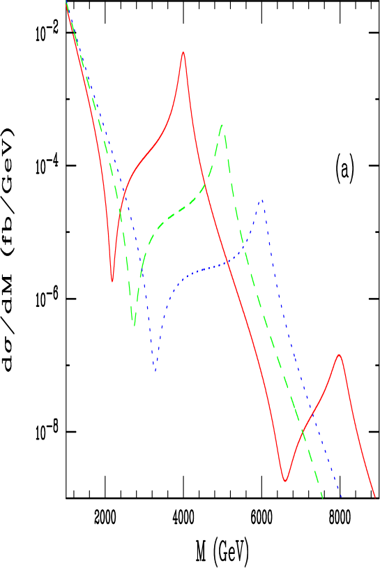
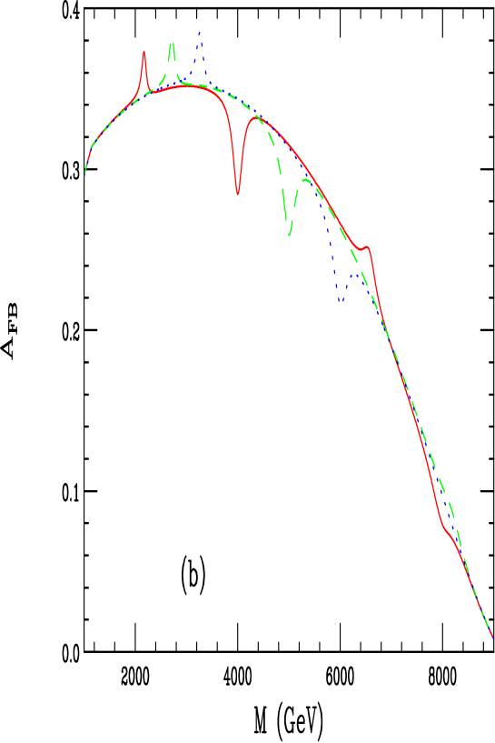
Figure 1: (a)Cross section and (b) Forward-Backward asymmetry for Drell-Yan production of the degenerate neutral KK excitations $Z^{(n)}$ and $\gamma^{(n)}$ as a function of the dilepton invariant mass at the LHC assuming one extra dimension and naive coupling values with $1/R$=4(5, 6) TeV corresponding to the solid(dashed, dotted) curve. The second excitation is only shown for the case of $1/R=4$ TeV.

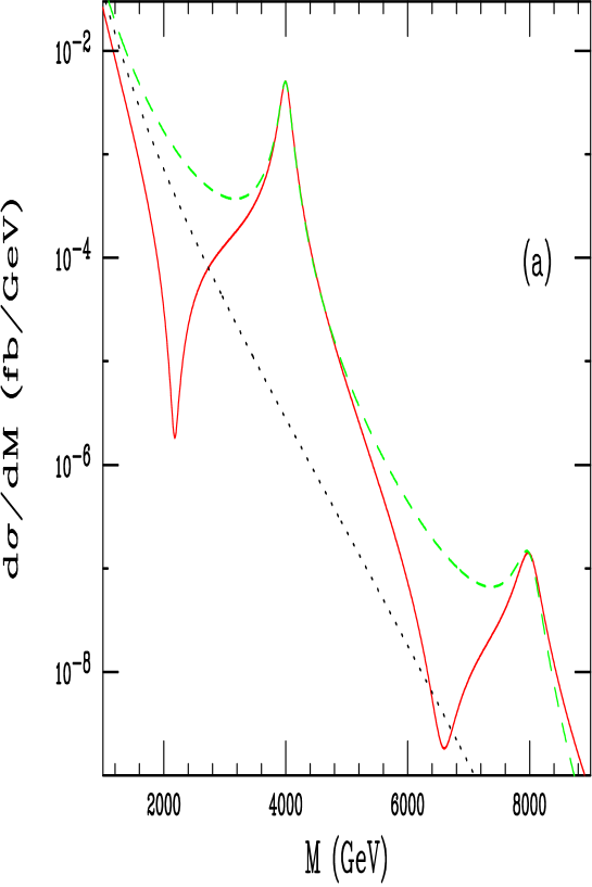
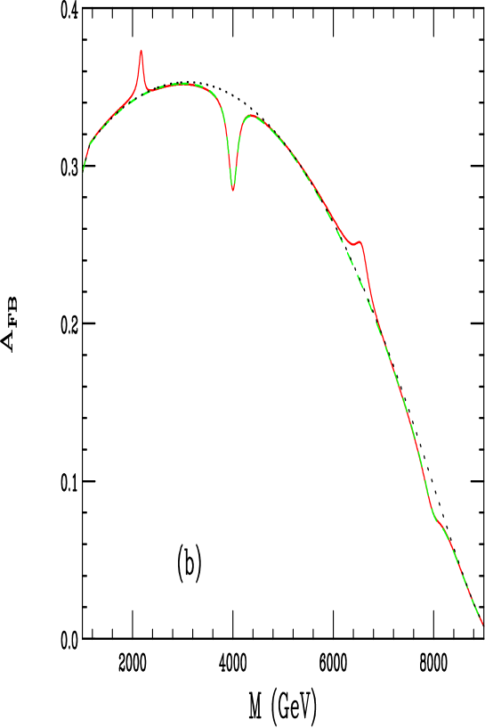
Figure 2: Same as the previous plot for the case of $1/R=4$ TeV(solid) but now also showing both the SM result for comparison(dots) as well as the alternative excitation curve for the case where the naive couplings are altered as in the scenario of Arkani-Hamed and Schmaltz(dashed)[7].

At the LHC in the case of one extra dimension (or two extra dimensions with $n_{max}$ very small) we are left with the somewhat more subtle KK signature of degenerate $\gamma^{(1)}$, $Z^{(1)}$, $W^{(1)}$ and $g^{(1)}$ states. However, even this signature may not be realized experimentally as the $g^{(1)}$ resonance may be easily washed out due to both experimental jet energy resolution and the resonance’s very large width to mass ratio[6] when its mass lies in the range above $\simeq 4$ TeV. More than likely a shoulder-like structure would remain visible but would be difficult to interpret[16]. We are thus left with a degenerate set of $\gamma^{(1)}$, $Z^{(1)}$, and $W^{(1)}$ as a potential signal for KK scenarios at the LHC. Unfortunately a degenerate pair of new gauge bosons $Z^{\prime},W^{\prime}$ is not a unique signal for KK models as many extended electroweak theories predict[17] such a situation. Of course the single ‘resonance’ in the $\ell^{+}\ell^{-}$ channel in the KK case is actually a superposition of both the $\gamma^{(1)}$ and $Z^{(1)}$ and not just a $Z^{\prime}$. Our claim here is that the LHC will not be able to distinguish these two possibilities given the rather small number of available observables due to the rather limited statistics.

To clarify this situation let us consider the results displayed in Figs. 1 and 2 for the case of one extra dimension. In Fig.1 we show the production cross sections and Forward-Backward Asymmetries, $A_{FB}$, in the $\ell^{+}\ell^{-}$ channel with inverse compactification radii of 4, 5 and 6 TeV. In calculating these cross sections we have assumed that the KK excitations have their naive couplings and can only decay to the usual fermions of the SM. Additional decay modes can lead to appreciably lower cross sections so that we cannot use the peak heights to determine the degeneracy of the KK state. Note that in the 4 TeV case, which is essentially as small a mass as can be tolerated by the present data on precision measurements, the second KK excitation is visible in the plot. We see several things from these figures. First, we can easily estimate the total number of events in the resonance regions associated with each of the peaks assuming the canonical integrated luminosity of $100fb^{-1}$ appropriate for the LHC; we find $\simeq 300(32,3,0.02)$ events corresponding to the 4(5,6,8) TeV resonances if we sum over both electron and muon final states and assume $100\%$ leptonic identification efficiencies. Clearly the 6 and 8 TeV resonances will not be visible at the LHC (though a modest increase of luminosity will allow the 6 TeV resonance to become visible) and we also verify our claim that only the first KK excitations will be observable. In the case of the 4 TeV resonance there is sufficient statistics that the KK mass will be well measured and one can also imagine measuring $A_{FB}$ since the final state muon charges can be signed. Given sufficient statistics, a measurement of the angular distribution would demonstrate that the state is indeed spin-1 and not spin-0 or spin-2. However, for such a heavy resonance it is unlikely that much further information could be obtained about its couplings and other properties and the values of $A_{FB}$ alone cannot determine whether this resonance is composite no matter how much statistics is available. In fact the conclusion of $Z^{\prime}$ analyses[18] is that coupling information will be essentially impossible to obtain for $Z^{\prime}$-like resonances with masses in excess of 1-2 TeV at the LHC. Furthermore, the lineshape of the 4 TeV resonance will be difficult to measure in detail due to both the limited statistics and energy smearing. Thus we will never know from LHC data alone whether the first KK resonance has been discovered or, instead, some extended gauge model scenario has been realized.

It is often stated[6] that the sharp dip in the cross section at an approximate dilepton pair invariant mass of $\simeq M_{1}/2$ will be a unique signal for the KK scenario. However, there are several difficulties with this claim. First, it is easy to construct alternative models with one extra dimension wherein either the leptonic or hadronic couplings of the odd excitations have opposite sign to the usual assignment, as in the model of Arkani-Hamed and Schmaltz(AS)[7], since the fermions lie at different fixed points on the wall. Here we consider the specific scenario where the quarks and leptons are at opposite fixed points. In this case the excitation curves will look quite different as shown in Fig.2 where we see that the dip below the resonance has now essentially disappeared. Second, even if the dip is present it will be difficult to observe directly given the LHC integrated luminosity. The reason here is that if we examine a 100 GeV wide bin around the location of the apparent minimum, the SM predicts only 5 events to lie in this bin assuming an integrated luminosity of 100 $fb^{-1}$. To prove that any dip is present we would need to demonstrate that the event rate is significantly below the SM value which would appear to be rather difficult if at all possible. Thus we stick to our conclusion that the LHC cannot distinguish between an ordinary $Z^{\prime}$ and the degenerate $Z^{(1)}/\gamma^{(1)}$ resonance and we must turn elsewhere to resolve this ambiguity.

4 Lepton Colliders Below the Resonance

It is well-known that future $e^{+}e^{-}$ linear colliders(LC) operating in the center of mass energy range $\sqrt{s}=0.5-1.5$ TeV will be sensitive to indirect effects arising from the exchange of new $Z^{\prime}$ bosons with masses typically 6-7 times greater than $\sqrt{s}$[18]. Furthermore, analyses have shown that with enough statistics the couplings of the new $Z^{\prime}$ to the SM fermions can be extracted[19] in a rather precise manner, especially when the $Z^{\prime}$ mass is already approximately known from elsewhere, e.g., the LHC. (If the $Z^{\prime}$ mass is not known then measurements at several distinct values of $\sqrt{s}$ can be used to extract both the mass as well as the corresponding couplings[20].)

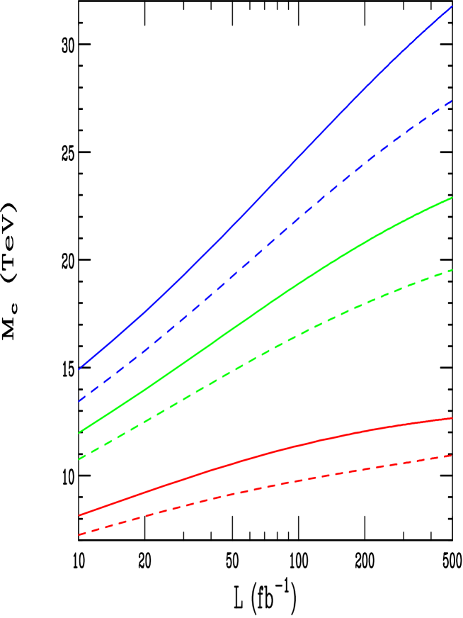
Figure 3: Search reach, $M_{c}$, for the first $Z^{(1)}/\gamma^{(1)}$ excited state as a function of the integrated luminosity assuming $e^{+}e^{-}$ collider center of mass energies, from top to bottom, of 1.5, 1, 0.5 TeV. One extra dimension is assumed. The solid curves correspond to the case of ‘conventional’ couplings while the dashed curves are for the case of the AS scenario[7].

In the present situation, we imagine that the LHC has discovered and determined the mass of a $Z^{\prime}$-like resonance in the 4-6 TeV range. Can the LC tell us anything about this object? The first question to ask is whether the LC can indirectly detect this excitation via the $e^{+}e^{-}\rightarrow f\bar{f}$ channels. (More precisely, can it probe the entire tower of KK states of which the 4-6 TeV object is the lowest lying one.) To address this issue we have repeated the Monte Carlo analyses in [18, 19, 20] and have asked for the search reach for the first KK excitation as a function of integrated luminosity. To obtain our results we have combined the $f=e,\mu,\tau,b,c$ and $t$ final states, assumed $90\%$ beam polarization and included angle cuts, initial state radiation, identification efficiencies and systematics associated with the overall luminosity determination. The angular distribution of the various cross sections, the Left-Right Asymmetries, $A_{LR}^{f}$, and the polarization of the $\tau$’s in the final state are simultaneously combined in this fit. The search reaches are shown in Fig.3 for the case of one extra dimension and assume the conventional naive coupling relationships. Note that the reach is as much as three times greater than that for a more conventional $Z^{\prime}$. The reasons for this are as follows: ($i$) the couplings of the KK excitations are larger than those of their SM partners by $\sqrt{2}$, ($ii$) the complete towers contribute to these deviations and ($iii$) both $\gamma^{(n)}$ and $Z^{(n)}$ towers are present and add coherently. If we allow for more than one extra dimension, cutting off the KK sum by either of the techniques described above, it is clear that our resulting reach will be significantly higher in mass due to the greater number of states and the larger couplings involved.

Figure 4: Fitted values of the parameters $v_{l}$ and $a_{l}$ following the procedures described in the text for a 4 TeV KK excitation at a 500 GeV $e^{+}e^{-}$ collider. The contour described the $95\%$ CL region with the best fit value as a diamond. The normalization is such that the corresponding SM $Z$ boson’s axial-vector coupling to the electron is -1/2.

The next step would be to use the LC to extract the couplings of the apparent resonance discovered by the LHC; we find that it is sufficient for our arguments to do this solely for the leptonic channels. The idea is the following: we measure the deviations in the differential cross sections and angular dependent $A_{LR}^{f}$’s for the three lepton generations and combine those with $\tau$ polarization data. Assuming lepton universality(which would be observed in the LHC data anyway), that the resonance mass is well determined, and that the resonance is an ordinary $Z^{\prime}$ we perform a fit to the hypothetical $Z^{\prime}$ coupling to leptons, $v_{l},a_{l}$. To be specific, let us consider the case of only one extra dimension with a 4 TeV KK excitation and employ a $\sqrt{s}=500$ GeV collider with an integrated luminosity of 200 $fb^{-1}$. The result of performing these fits is shown in Fig.4 from which we see that the coupling values are ‘well determined’ (i.e., the size of the allowed region we find is quite small) by the fitting procedure as we would have expected from previous analyses of $Z^{\prime}$ couplings extractions at linear colliders[18, 19, 20]. We note that identical results are obtained for this analysis if we assume that the KK excitations are of the type discussed by Arkani-Hamed and Schmaltz[7].

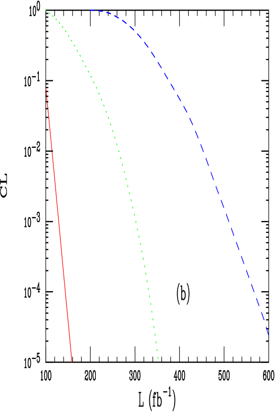
Figure 5: CL as a function of the integrated luminosity resulting from the coupling fits following from the analysis discussed in the text for both (a) a 500 GeV or a (b) 1 TeV $e^{+}e^{-}$ collider. In (a) the solid(dash-dotted,dotted) curve corresponds to a first KK excitation mass of 4(5,6) TeV. In (b) the solid(dotted,dashed) curve corresponds to a first KK mass of 5(6,7) TeV.

The only problem with the fit shown in the figure is that the $\chi^{2}$ is very large leading to a very small confidence level, i.e., $\chi^{2}/d.o.f=95.06/58$ or P=CL=$1.55\times 10^{-3}$! (We note that this result is not very sensitive to the assumption of $90\%$ beam polarization; $70\%$ polarization leads to almost identical results.) For an ordinary $Z^{\prime}$ it has been shown that fits of much higher quality, based on confidence level values, are obtained by this same procedure. Increasing the integrated luminosity can be seen to only make matters worse. Fig.5 shows the results for the CL following the above approach as we vary both the luminosity and the mass of the first KK excitation at both 500 GeV and 1 TeV $e^{+}e^{-}$ linear colliders. From this figure we see that the resulting CL is below $\simeq 10^{-3}$ for a first KK excitation with a mass of 4(5,6) TeV when the integrated luminosity at the 500 GeV collider is 200(500,900)$fb^{-1}$ whereas at a 1 TeV for excitation masses of 5(6,7) TeV we require luminosities of 150(300,500)$fb^{-1}$ to realize this same CL. Barring some unknown systematic effect the only conclusion that one could draw from such bad fits is that the hypothesis of a single $Z^{\prime}$, and the existence of no other new physics, is simply wrong. If no other exotic states are observed below the first KK mass at the LHC this result would give very strong indirect evidence that something more unusual that a conventional $Z^{\prime}$ had been found. The problem from the experimental point of view would be to wonder what fitting hypothesis to try next as there are so many possibilities to try. For example, one can imagine trying a two $Z^{\prime}$ scenario with the first at 4 TeV, as discovered by the LHC, and with the second $Z^{\prime}$ at 6 or more TeV, beyond the range of the LHC. Eventually one might try repeating the above fitting procedure allowing for two essentially degenerate new gauge bosons with different leptonic couplings could then be shown to yield a good fit to the data. Furthermore, it is clear from the discussion that all of the analysis performed above will go through in an almost identical manner in the case of more than one extra dimension yielding qualitatively similar results.

5 Lepton Colliders on (and near) the Resonance

In order to be completely sure of the nature of the first KK excitation, we must produce it directly at a higher energy lepton collider and sit on and near the peak of the KK resonance. To reach this mass range will most likely require either CLIC technology[21] or a Muon Collider[22]. Recall that the mass of the KK resonance is already quite well known from data from the LHC so that the center of mass energy of the Muon Collider can be chosen near this value.

The first issue to address is the quality of the degeneracy of the $\gamma^{(1)}$ and $Z^{(1)}$ states. If any part of the Higgs boson(s) whose vacuum expectation(s) value breaks the SM down to $U(1)$ is on the ‘wall’ then the SM $Z$ will mix with the $Z^{(n)}$ slightly shifting all their masses; due to the remaining $U(1)$ gauge invariance this will not happen to the $\gamma^{(n)}$ thus implying a slight difference between the $\gamma^{(1)}$ and $Z^{(1)}$ masses. Based on the analyses in Ref.[9] we can get an idea of the maximum possible size of this fractional mass shift and we find it to be of order $\sim M_{Z}^{4}/M_{Z^{(1)}}^{4}$, an infinitesimal quantity for KK masses in the several TeV range. Thus even when mixing is included we find that the $\gamma^{(1)}$ and $Z^{(1)}$ states remain very highly degenerate so that even detailed lineshape measurements may not be able to distinguish the $\gamma^{(1)}/Z^{(1)}$ composite state from that of a $Z^{\prime}$. We thus must turn to other parameters in order to separate these two cases.

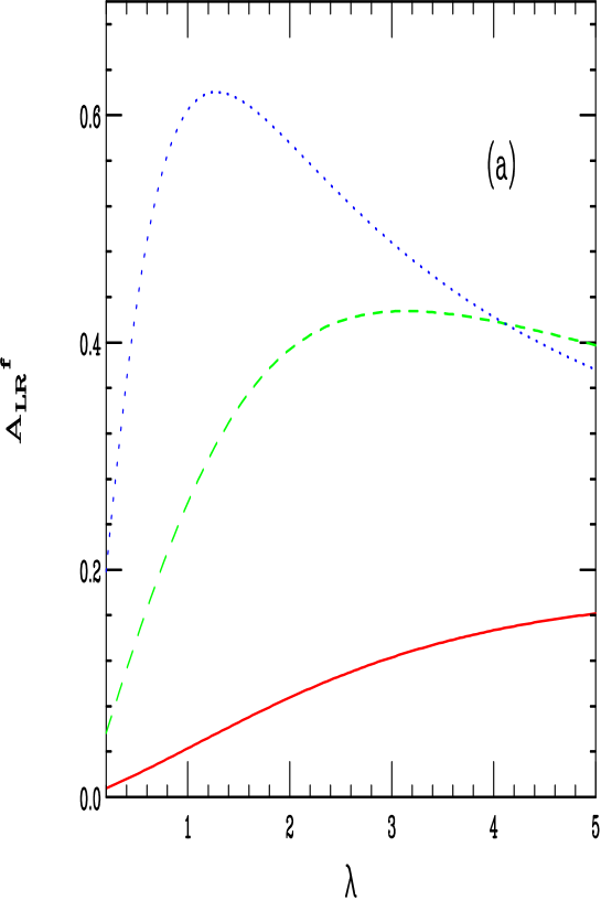
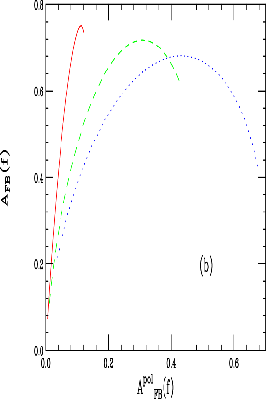
Figure 6: (a) $A_{LR}^{f}$ as a function of the parameter $\lambda$ for $f=\ell$(solid), $f=c$(dashed) and $f=b$(dots). (b) Correlations between on-peak observables for the same three cases as shown in (a). $\lambda$ varies from 0.2 to 5 along each curve.

Sitting on the resonance there are a very large number of quantities that can be measured: the mass and apparent total width, the peak cross section, various partial widths and asymmetries etc. From the $Z$-pole studies at SLC and LEP, we recall a few important tree-level results which we would expect to apply here as well provided our resonance is a simple $Z^{\prime}$. First, we know that the value of $A_{LR}=[A_{e}=2v_{e}a_{e}/(v_{e}^{2}+a_{e}^{2})]$, as measured on the $Z$ by SLD, does not depend on the fermion flavor of the final state and second, that the relationship $A_{LR}\cdot A_{FB}^{pol}(f)=A_{FB}^{f}$ holds, where $A_{FB}^{pol}(f)$ is the polarized Forward-Backward asymmetry as measured for the $Z$ at SLC and $A_{FB}^{f}$ is the usual Forward-Backward asymmetry. The above relation is seen to be trivially satisfied on the $Z$(or on a $Z^{\prime}$) since $A_{FB}^{pol}(f)={3\over 4}A_{f}$ and $A_{FB}^{f}={3\over 4}A_{e}A_{f}$. Both of these relations are easily shown to fail in the present case of a ‘dual’ resonance though they will hold if only one particle is resonating.

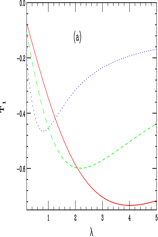
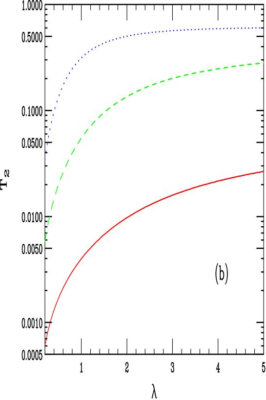
Figure 7: The quantities (a)$T_{1}$ and (b)$T_{2}$ as functions of the parameter $\lambda$. The curves are labelled as in the previous figure.

A short exercise shows that in terms of the couplings to $\gamma^{(1)}$, which we will call $v_{1},a_{1}$, and $Z^{(1)}$, now called $v_{2},a_{2}$, these same observables can be written as

$$A_{FB}^{f} = {3\over 4}{A_{1}\over D}$$

$$A_{FB}^{pol}(f) = {3\over 4}{A_{2}\over D}$$

$$A_{LR}^{f} = {A_{3}\over D}\,,$$ (3)

where $f$ labels the final state fermion and we have defined the coupling combinations

$$D = (v_{1}^{2}+a_{1}^{2})_{e}(v_{1}^{2}+a_{1}^{2})_{f}+R^{2}(v_{2}^{2}+a_{2}^{2})_{e}(v_{2}^{2}+a_{2}^{2})_{f}+2R(v_{1}v_{2}+a_{1}a_{2})_{e}(v_{1}v_{2}+a_{1}a_{2})_{f}$$

$$A_{1} = (2v_{1}a_{1})_{e}(2v_{1}a_{1})_{f}+R^{2}(2v_{2}a_{2})_{e}(2v_{2}a_{2})_{f}+2R(v_{1}a_{2}+v_{2}a_{1})_{e}(v_{1}a_{2}+v_{2}a_{1})_{e}$$

$$A_{2} = (2v_{1}a_{1})_{f}(v_{1}^{2}+a_{1}^{2})_{e}+R^{2}(2v_{2}a_{2})_{f}(v_{2}^{2}+a_{2}^{2})_{e}+2R(v_{1}a_{2}+v_{2}a_{1})_{f}(v_{1}v_{2}+a_{1}a_{2})_{e}$$

$$A_{3} = (2v_{1}a_{1})_{e}(v_{1}^{2}+a_{1}^{2})_{f}+R^{2}(2v_{2}a_{2})_{e}(v_{2}^{2}+a_{2}^{2})_{f}+2R(v_{1}a_{2}+v_{2}a_{1})_{e}(v_{1}v_{2}+a_{1}a_{2})_{f}\,,$$ (4)

with $R$ is the ratio of widths $R=\Gamma_{1}/\Gamma_{2}$ and the $v_{1,2i},a_{1,2i}$ are the appropriate couplings for electrons and fermions $f$. Note that when $R$ gets either very large or very small we recover the usual ‘single resonance’ results. Examining these equations we immediately note that $A_{LR}^{f}$ is now flavor dependent and that the relationship between observables is no longer satisfied:

$$A_{LR}^{f}\cdot A_{FB}^{pol}(f)\neq A_{FB}^{f}\,,$$ (5)

which clearly tells us that we are actually producing more than one resonance. Note that the numerical values of all of these asymmetries, being only proportional to ratios of various couplings, are independent of how much damping the KK couplings experience due to the stiffness of the wall. In what follows we will limit ourselves to electroweak observables whose values are independent of the overall normalization of the couplings and the potential exotic decay modes of the first KK excitation.

Of course we need to verify that these single resonance relations are numerically badly broken before clear experimental signals for more than one resonance can be claimed. Statistics will not be a problem with any reasonable integrated luminosity since we are sitting on a resonance peak and certainly millions of events will be collected. Assuming decays to only SM final states we estimate that with an integrated luminosity of 100 $fb^{-1}$ a sample of approximately half a million lepton pairs will be obtainable for each flavor. In principle, to be as model independent as possible in a numerical analysis, we should allow the widths $\Gamma_{i}$ to be greater than or equal to their SM values as such heavy KK states may decay to SM SUSY partners as well as to presently unknown exotic states. Since the expressions above only depend upon the ratio of widths, we let $R=\lambda R_{0}$ where $R_{0}$ is the value obtained assuming that the KK states have only SM decay modes. We then treat $\lambda$ as a free parameter in what follows and explore the range $1/5\leq\lambda\leq 5$. Note that as we take $\lambda\rightarrow 0(\infty)$ we recover the limit corresponding to just a $\gamma^{(1)}(Z^{(1)})$ being present.

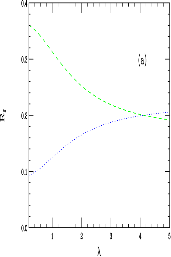
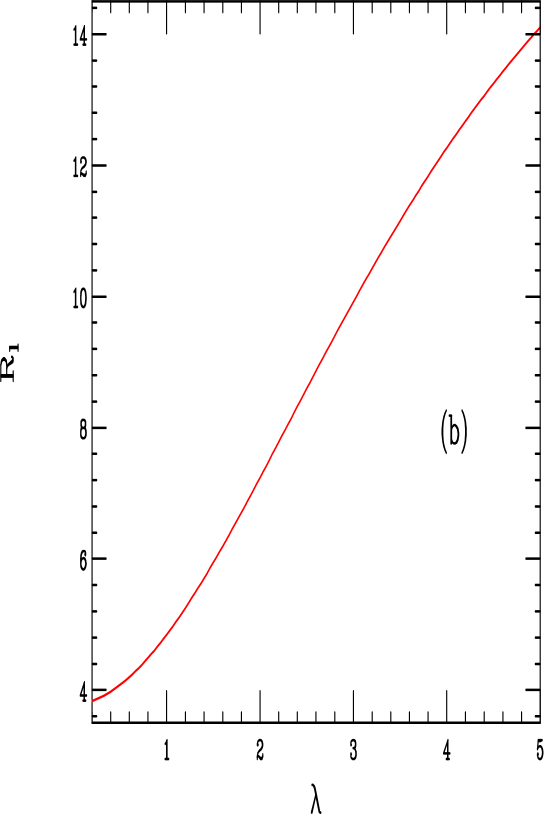
Figure 8: (a) The ratios of the $\bar{b}b$(dots) and $\bar{c}c$ cross sections to that for all hadrons on top of the 4 TeV KK excitation. (b) The ratio of the hadron cross section to that for leptons on the peak of the KK excitation.

In Fig.6 we display the flavor dependence of $A_{LR}^{f}$ as a functions of $\lambda$. Note that as $\lambda\rightarrow 0$ the asymmetries vanish since the $\gamma^{(1)}$ has only vector-like couplings. In the opposite limit, for extremely large $\lambda$, the $Z^{(1)}$ couplings dominate and a common value of $A_{LR}$ will be obtained. It is quite clear, however, that over the range of reasonable values of $\lambda$, $A_{LR}^{f}$ is quite obviously flavor dependent. We also show in Fig.6 the correlations between the observables $A_{FB}^{pol}(f)$ and $A_{FB}(f)$ which would be flavor independent if only a single resonance were present. From the figure we see that this is clearly not the case. Note that although $\lambda$ is an a priori unknown parameter, once any one of the electroweak observables are measured the value of $\lambda$ will be directly determined. Once $\lambda$ is fixed, then the values of all of the other asymmetries, as well as the ratios of various partial decay widths, are all completely fixed for the KK resonance with uniquely predicted values.

In order to further numerically probe the breakdown of the relationship between the on-resonance electroweak observables in Eq. (5) we consider two related quantities:

$$T_{1} = A_{LR}^{f}\cdot A_{FB}^{pol}(f)-A_{FB}^{f}$$

$$T_{2} = {A_{LR}^{f}\cdot A_{FB}^{pol}(f)\over{A_{FB}^{f}}}\,,$$ (6)

the first of which should vanish while the second should be equal to unity independently of the fermion flavor if only a single resonance were present. In this case, both these variables have values far away from these expectations and are shown in Fig.7 as functions of $\lambda$.

For completeness, we show in Fig.8 the ratio of partial widths $R_{b,c}=\Gamma_{b,c}/\Gamma_{had}$ and $R_{\ell}=\Gamma_{had}/\Gamma_{\ell}$. Once the parameter $\lambda$ is fixed the corresponding values of these observables become uniquely determined. The values of these quantities will help to pin down the nature of this resonance as a combined $Z^{(1)}/\gamma^{(1)}$ KK excitation. Recall that once $\lambda$ is fixed, then the values of all of the other asymmetries, as well as the ratios of various partial decay widths, are all completely fixed for the KK resonance with uniquely predicted values. These can then be compared to the data extracted by the Muon Collider and will demonstrate that the double resonance is composed of an excited photon and $Z$, the hallmark of the KK scenario.

In Figs.9 and 10 we show that although on-resonance measurements of the electroweak observables, being quadratic in the $Z^{(1)}$ and $\gamma^{(1)}$ couplings, will not distinguish between the conventional KK scenario and that of the AS, the data below the peak in the hadronic channel will easily allow such a separation. The cross section and asymmetries for $e^{+}e^{-}\rightarrow\mu^{+}\mu^{-}$ (or vice versa) is, of course, the same in both cases. The combination of on and near resonance measurements will thus completely determine the nature of the resonance. Off-resonance measurements can be made possible through the use of ‘radiative returns’ wherein the emission of initial state photons allow one to perform as scan at all energies below the collider design $\sqrt{s}$.

We note that all of the above analysis will go through essentially unchanged in any qualitative way when we consider the case of the first KK excitation in a theory with more than one extra dimension.

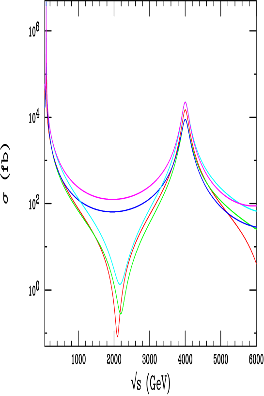
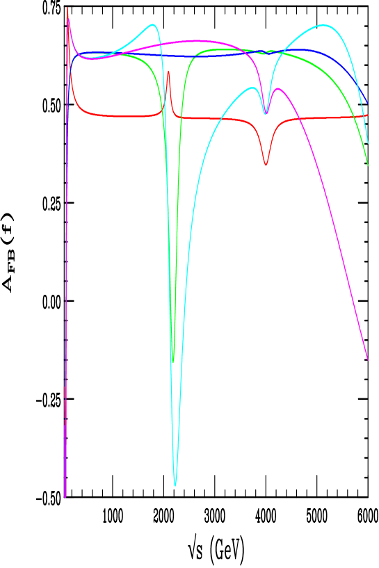
Figure 9: Cross sections and $A_{FB}$ for $e^{+}e^{-}\rightarrow\mu^{+}\mu^{-}$ $b\bar{b}$ and $c\bar{c}$ at high energy lepton colliders in both the ‘conventional’ scenario and that of AS[7]. The red curve applies for the $\mu$ final state in either model whereas the green(blue) and cyan(magenta) curves label the $b$ and $c$ final states for the ‘conventional’(AS) scenario.

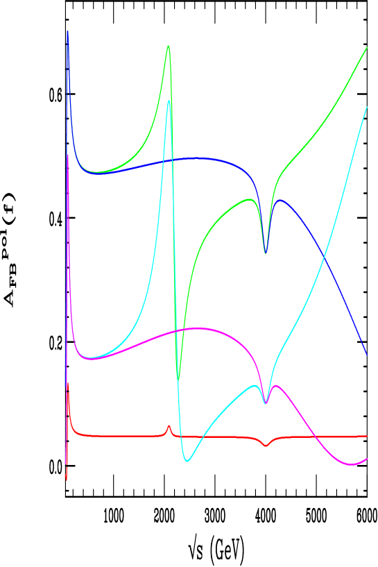
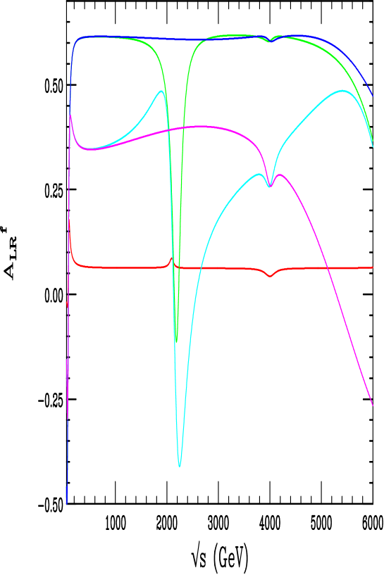
Figure 10: Same as the previous figure but now for the observables $A_{LR}^{f}$ and $A_{FB}^{pol}(f)$.

6 Summary and Conclusions

Present data strongly indicates that if KK excitations of the SM gauge bosons exist then the masses of the first tower excitations probably lie near or above 4 TeV if there is only one extra dimension and the KK states have naive couplings to the SM fermions. For KK masses in the 4-6 TeV range, the LHC will have sufficient luminosity to allow detection of these new particles although, for the case of the gluon excitation, any resonance-like structure might be too smeared out to be observable as a peak. Unfortunately, however, the second set of SM excitations will be far too heavy to be produced and thus the exciting ‘recurring resonance’ signature one anticipates from KK theories is lost. In addition, since the first excitations are so massive, their detailed properties are not discernable so that the KK excitations of the $Z$ and $\gamma$ will appear to be a single $Z^{\prime}$ peak. Thus as far as experiment at the LHC can determine we are left with what appears to be a degenerate $Z^{\prime}/W^{\prime}$ pair, something which can occur in many extended electroweak models. In this paper we have sought to resolve this problem based on information that can be gathered at lepton colliders in operation both far below and in the neighborhood of the first KK excitation mass. To perform this task and to solidify the above arguments we have taken the following steps obtaining important results along the way:

• All constraints on the common mass, $M_{1}$, of the first SM KK excitations, apart from direct collider searches, rely on a two step process involving a parameter (or set of parameters) such as $V$ introduced in Eq.(1). First, given a set of data and the assumption that multiple new physics sources are not conspiring to distort the result, a bound on $V$ is obtained. The problem lies in the second step, i.e., converting the bound on $V$ into one on $M_{1}$. This is usually done in the case of one extra dimension where one naively sums over the entire tower of KK modes which converges numerically. However, we know that this convergence property no longer holds when we consider the case of more than one extra dimension which makes $V$ difficult to interpret in a more general context. Furthermore, the exact nature of the sum depends on the details of the compactification scenario when we extend the analysis to the case of more than one dimension. As specific examples we explored the case of two extra dimensions assuming either a $S^{1}/Z_{2}\times S^{1}/Z_{2}$, $Z_{3}$ or $Z_{6}$ compactification employing both a direct cut off of the tower sum as well as the better motivated exponential damping of the higher mode couplings. Depending upon the details of this cut off procedure in the case of more than one extra dimension we have shown that the lower limit on the mass of the first KK excitation arising from the bound on $V$ may lie outside of the range accessible to the LHC unless the parameter controlling the cut off, $n_{max}$, is quite small. Neither of these cut off approaches significantly alter our conclusions for the case of only one extra dimension.

• Given the mass of the apparent $Z^{\prime}$ resonance from the LHC, a low energy lepton collider can be used to attempt an extraction of it’s leptonic couplings from a simultaneous fit to a number of distinct observables. While we demonstrated that a reasonably small region of the allowed parameter space will be selected by the fit, the confidence level was found to be very small in contrast to what happens in the case of an ordinary $Z^{\prime}$. For example, a 500 GeV collider with an integrated luminosity of $\simeq 200$ $fb^{-1}$ probing a KK excitation with a mass of 4 TeV would obtain a fit probability of only $\simeq 10^{-3}$. This analysis was then generalized for both other KK masses and for a 1 TeV collider. We then argued that such an analysis would strongly indicate that the apparent $Z^{\prime}$ observed by the LHC is not a single resonance. However, a fit allowing for the existence of a degenerate double resonance would yield an acceptable $\chi^{2}$.

• Employing a lepton collider with sufficient center of mass energy, data can be taken at or near the first KK resonance. In this case we demonstrated that the familiar relationships between electroweak observables, in particular the various on-pole asymmetries, no longer hold in the presence of two degenerate resonances. For example, $A_{LR}$ now becomes flavor dependent and the factorization relationship $A_{LR}\cdot A_{FB}^{pol}(f)=A_{FB}^{f}$ was demonstrated to fail. The values of all of the on-pole observables was shown to be uniquely determined once the value of a single parameter, $\lambda$, which describes the relative total widths of the $\gamma^{(1)}$ and $Z^{(1)}$, is known. If both KK excitations only decay to SM particles, then $\lambda=1$. Furthermore, we showed that data taken off resonance can be used to distinguish among various models of the KK couplings and the localization of the fermions on the wall.

It is clear both the LHC and lepton colliders will be necessary to explore the physics of KK excitations.

Acknowledgements

The author would like to thank J.L. Hewett, J. Wells, I. Antoniadis, P. Nath, N. Arkani-Hamed, H. Davoudiasl, M. Schmaltz, Y. Grossman, M. Masip and F. del Aguila for discussions related to this work. He would also like to thank the members of the CERN Theory Division, where this work was begun, for their hospitality.

References

- [1] I. Antoniadis, Phys. Lett. B246, 377 (1990); I. Antoniadis, C. Munoz and M. Quiros, Nucl. Phys. B397, 515 (1993); I. Antoniadis and K. Benalki, Phys. Lett. B326, 69 (1994); I. Antoniadis, K. Benalki and M. Quiros, Phys. Lett. B331, 313 (1994); K. Benalki, Phys. Lett. B386, 106 (1996).
- [2] N. Arkani-Hamed, S. Dimopoulos and G. Dvali, Phys. Lett. B429, 263 (1998) and Phys. Rev. D59, 086004 (1999); I. Antoniadis, N. Arkani-Hamed, S. Dimopoulos and G. Dvali, Phys. Lett. B436, 257 (1998;)N. Arkani-Hamed, S. Dimopoulos and J. March-Russell, hep-th/9809124; P.C. Argyres, S. Dimopoulos and J. March-Russell, Phys. Lett. B441, 96 (1998); Z. Berezhiani and G. Dvali, hep-ph/9811378; N. Arkani-Hamed and S. Dimopoulos, hep-ph/9811353; Z. Kakushadze, hep-th/9811193 and hep-th/9812163; N. Arkani-Hamed et al., hep-ph/9811448; G. Dvali and S.-H.H. Tye, hep-ph/9812483. See also, G. Shiu and S.-H. H. Tye, Phys. Rev. D58, 106007 (1998); Z. Kakushadze and S.-H. H. Tye, hep-th/9809147; J. Lykken, Phys. Rev. D54, 3693 (1996); E. Witten, Nucl. Phys. B471, 135 (1996); P. Horava and E. Witten, Nucl. Phys. B460, 506 (1996) and Nucl. Phys. B475, 94 (1996).
- [3] For an incomplete list, see G.F. Giudice, R. Rattazzi and J.D. Wells, Nucl. Phys. B544, 3 (1999), hep-ph/9811291; E.A. Mirabelli, M. Perelstein and M.E. Peskin, Phys. Rev. Lett. 82, 2236 (1999), hep-ph/9811337; T. Han, J.D. Lykken and R. Zhang, Phys. Rev. D59, 105006 (1999), hep-ph/9811350; J.L. Hewett, Phys. Rev. Lett. 82, 4765 (1999), hep-ph/9811356; N. Arkani-Hamed, S. Dimopoulos, G. Dvali and J. March-Russell, hep-ph/9811448; N. Arkani-Hamed and S. Dimopoulos, hep-ph/9811353; K. Benakli and S. Davidson, hep-ph/9810280; Z. Berezhiani and G. Dvali, Phys. Lett. B450, 24 (1999), hep-ph/9811378; K.R. Dienes, E. Dudas and T. Gherghetta, hep-ph/9811428; Z. Kakushadze, Nucl. Phys. B548, 205 (1999), hep-th/9811193; P. Mathews, S. Raychaudhuri and K. Sridhar, Phys. Lett. B450, 343 (1999), hep-ph/9811501; Z. Kakushadze, hep-th/9812163; P. Mathews, S. Raychaudhuri and K. Sridhar, Phys. Lett. B455, 115 (1999), hep-ph/9812486; T.G. Rizzo, Phys. Rev. D59, 115010 (1999), hep-ph/9901209; A.E. Faraggi and M. Pospelov, Phys. Lett. B458, 237 (1999); S.Y. Choi, J.S. Shim, H.S. Song, J. Song and C. Yu, Phys. Rev. D60, 013007 (1999), hep-ph/9901368; I. Antoniadis, hep-ph/9904272; M. Dine, hep-ph/9905219; K. Agashe and N.G. Deshpande, Phys. Lett. B456, 60 (1999), hep-ph/9902263; T.G. Rizzo, hep-ph/9902273; M.L. Graesser, hep-ph/9902310; Z. Silagadze, hep-ph/9907328 and hep-ph/9908208; Z. Kakushadze, Nucl. Phys. B551, 549 (1999), hep-th/9902080; T. Banks, M. Dine and A. Nelson, JHEP 06, 014 (1999), hep-th/9903019; K. Cheung and W. Keung, hep-ph/9903294; S. Cullen and M. Perelstein, Phys. Rev. Lett. 83, 268 (1999); T.G. Rizzo, Phys. Rev. D60, 075001 (1999); D. Atwood, S. Bar-Shalom and A. Soni, hep-ph/9903538; C. Balazs, H. He, W.W. Repko, C.P. Yuan and D.A. Dicus, hep-ph/9904220; P. Mathews, S. Raychaudhuri and K. Sridhar, hep-ph/9904232; A.K. Gupta, N.K. Mondal and S. Raychaudhuri, hep-ph/9904234; G. Shiu, R. Shrock and S.H. Tye, Phys. Lett. B458, 274 (1999); K. Cheung, hep-ph/9904266; L.J. Hall and D. Smith, hep-ph/9904267; H. Goldberg, hep-ph/9904318; K.Y. Lee, H.S. Song and J. Song, hep-ph/9904355; T.G. Rizzo, hep-ph/9904380; H. Davoudiasl, hep-ph/9904425; K. Yoshioka, hep-ph/9904433; K. Cheung, Phys. Lett. B460, 383 (1999); K.Y. Lee, H.S. Song, J. Song and C. Yu, hep-ph/9905227; X. He, hep-ph/9905295; P. Mathews, P. Poulose and K. Sridhar, hep-ph/9905395; T. Han, D. Rainwater and D. Zeppenfeld, hep-ph/9905423; V. Barger, T. Han, C. Kao and R.J. Zhang, hep-ph/9905474; X. He, hep-ph/9905500; A. Pilaftsis, hep-ph/9906265; D. Atwood, S. Bar-Shalom and A. Soni, hep-ph/9906400; H. Davoudiasl, hep-ph/9907347; D. Bourilkov, hep-ph/9907380, T.G. Rizzo hep-ph/9907401; R.N. Mohapatra, S. Nandi and A. Perez-Lorenzana, hep-ph/9907520; A. Ioannisian and A. Pilaftsis, hep-ph/9907522; P. Das and S. Raychaudhuri, hep-ph/9908205; H.-C. Cheng and K.T. Matchev, hep-ph/9908328; O.J.P. Eboli, T. Han, M.B. Margo and P.G. Mercadante, hep-ph/9908358; X.-G. He, G.C. Joshi and B.H.J. McKellar, hep-ph/9908469; J. Lykken and S. Nandi, hep-ph/9908505; S. Chang, S. Tazawa and M. Yamaguchi, hep-ph/9908515; K. Cheung and G. Landsberg, hep-ph/9909218.
- [4] For an alternative to this scenario, see L. Randall and R. Sundrum, hep-ph/9905221 and hep-th/9906182; see also, W.D. Goldberg and M.B. Wise, hep-ph/9907218 and hep-ph/9907447.
- [5] K.R. Dienes, E. Dudas and T. Gherghetta, Phys. Lett. B436, 55 (1998) and Nucl. Phys. B537, 47 (1999); D. Ghilencea and G.C. Ross, Phys. Lett. B442, 165 (1998) and hep-ph/9908369; Z. Kakushadze, hep-th/9811193; C.D. Carone, hep-ph/9902407; P.H. Frampton and A. Rasin, Phys. Lett. B460, 313 (1999); A. Delgado and M. Quiros, hep-ph/9903400; A. Perez-Lorenzana and R.N. Mohapatra, hep-ph/9905137; H.-C. Cheng, B.A. Dobrescu and C.T. Hill, hep-ph/9906327; K. Hiutu and T. Kobayashi, hep-ph/9906431; D. Dimitru and S. Nandi, hep-ph/9906514; G.K. Leontaris and N.D. Tracas, hep-ph/9902368 and hep-ph/9908462.
- [6] I. Antoniadis, K. Benalki and M. Quiros, hep-ph/9905311; P. Nath, Y. Yamada and M. Yamaguchi, hep-ph/9905415; See also the first paper in Ref.[9].
- [7] N. Arkani-Hamed and M. Schmaltz, hep-ph/9903417; N. Arkani-Hamed, Y. Grossman and M. Schmaltz, to appear.
- [8] D0 Collaboration, S. Abachi et al.,Phys. Lett. B385, 471 (1996), Phys. Rev. Lett. 76, 3271 (1996) and Phys. Rev. Lett. 82, 29 (1999); CDF Collaboration, F. Abe et al., Phys. Rev. Lett. 77, 5336 (1996), Phys. Rev. Lett. 74, 2900 (1995) and Phys. Rev. Lett. 79, 2191 (1997).
- [9] T.G. Rizzo and J.D. Wells, hep-ph/9906234; P. Nath and M. Yamaguchi, hep-ph/9902323 and hep-ph/9903298; M. Masip and A. Pomarol, hep-ph/9902467; W.J. Marciano, hep-ph/9903451; L. Hall and C. Kolda, Phys. Lett. B459, 213 (1999); R. Casalbuoni, S. DeCurtis and D. Dominici, hep-ph/9905568; R. Casalbuoni, S. DeCurtis, D. Dominici and R. Gatto, hep-ph/9907355; A. Strumia, hep-ph/9906266; F. Cornet, M. Relano and J. Rico, hep-ph/9908299; C.D. Carone, hep-ph/9907362.
- [10] See T.G. Rizzo and J.D. Wells in Ref. [9].
- [11] M. Bando, T. Kugo, T. Noguchi and K. Yoshioka, hep-ph/9906549; see also the first paper in Ref. [6].
- [12] L. DiLella, talk given at the Recontres de Moriond: electroweak interactions and unified theories, 13-20 March 1999, Les Arcs, France.
- [13] J. Mnich, talk given at the International Europhysics Conference on High Energy Physics(EPS99), 15-21 July 1999, Tampere, Finland.
- [14] M. Swartz, M. Lancaster and D. Charlton talks given at the XIX International Symposium on Lepton and Photon Interactions, 9-14 August 1999, Stanford, California.
- [15] The best preliminary lower limit on the Higgs boson mass from the ALEPH Collaboration is 98.8 GeV. See, V. Ruhlmann-Kleider, talk given at the XIX International Symposium on Lepton and Photon Interactions, 9-14 August 1999, Stanford, California.
- [16] This is reasonably clear from the work of Nath, Yamada and Yamaguchi[6] before any mass resolution smearing is applied.
- [17] This is a common feature of the class of models wherein the usual of the SM is the result of a diagonal breaking of a product of two or more ’s. For a discussion of a few of these models, see H. Georgi, E.E. Jenkins, and E.H. Simmons, Phys. Rev. Lett. 62, 2789 (1989) and Nucl. Phys. B331, 541 (1990);V. Barger and T.G. Rizzo, Phys. Rev. D41, 946 (1990); T.G. Rizzo, Int. J. Mod. Phys. A7, 91 (1992); R.S. Chivukula, E.H. Simmons and J. Terning, Phys. Lett. B346, 284 (1995); A. Bagneid, T.K. Kuo, and N. Nakagawa, Int. J. Mod. Phys. A2, 1327 (1987) and Int. J. Mod. Phys. A2, 1351 (1987); D.J. Muller and S. Nandi, Phys. Lett. B383, 345 (1996); X.Li and E. Ma, Phys. Rev. Lett. 47, 1788 (1981) and Phys. Rev. D46, 1905 (1992); E. Malkawi, T.Tait and C.-P. Yuan, Phys. Lett. B385, 304 (1996); E. Malkawi and C.-P. Yuan, hep-ph/9906215.
- [18] For a review of new gauge boson physics at colliders and details of the various models, see J.L. Hewett and T.G. Rizzo, Phys. Rep. 183, 193 (1989); M. Cvetic and S. Godfrey, in Electroweak Symmetry Breaking and Beyond the Standard Model, ed. T. Barklow et al., (World Scientific, Singapore, 1995), hep-ph/9504216; T.G. Rizzo in New Directions for High Energy Physics: Snowmass 1996, ed. D.G. Cassel, L. Trindle Gennari and R.H. Siemann, (SLAC, 1997), hep-ph/9612440; A. Leike, hep-ph/9805494.
- [19] See, for example, A. Djouadi, A. Lieke, T. Riemann, D. Schaile and C. Verzegnassi, Z. Phys. C56, 289 (1992); J. Hewett and T. Rizzo, in Proceedings of the Workshop on Physics and Experiments with Linear Colliders, September 1991, Saariselkä, Finland, R. Orava ed., (World Scientific, Singapore, 1992) Vol. II, p.489, ibid p.501; G. Montagna et al., Z. Phys. C75, 641 (1997); F. del Aguila and M. Cvetic, Phys. Rev. D50, 3158 (1994); F. del Aguila, M. Cvetic and P. Langacker Phys. Rev. D52, 37 (1995); A. Lieke, Z. Phys. C62, 265 (1994); D. Choudhury, F. Cuypers and A. Lieke, Phys. Lett. B333, 531 (1994); S. Riemann in New Directions for High Energy Physics: Snowmass 1996, ed. D.G. Cassel, L. Trindle Gennari and R.H. Siemann, (SLAC, 1997), hep-ph/9610513; A. Lieke and S. Riemann, Z. Phys. C75, 341 (1997); T.G. Rizzo, hep-ph/9604420.
- [20] T.G. Rizzo, Phys. Rev. D55, 5483 (1997).
- [21] J.-P. Delahaye et al., The CLIC Study of a Multi-TeV Linear Collider, CERN/PS 99-005.
- [22] For a recent update, see C.M. Ankenbrandt et al., Status of Muon Collider Research and Development and Future Plans, Fermilab-Pub-98-179. See also B.J. King, hep-ex/9908041.