Event by Event Analysis and Entropy of Multiparticle Systems

Abstract

The coincidence method of measuring the entropy of a system, proposed some time ago by Ma, is generalized to include systems out of equilibrium. It is suggested that the method can be adapted to analyze multiparticle states produced in high-energy collisions.

05.30.-d, 13.85.Hd, 25.75.-q

1. Entropy, being one of the most important characteristics of a system with many degrees of freedom, is — in particular — an important characteristics of multiparticle production processes. In this context it abounds in analyses of dense hadronic matter and in discussions of various models of quark-gluon plasma [1].

Processes in which particles are produced can be considered as the so called dynamical systems [2, 3] in which — generally — entropy gets produced. Although application of the mathematical theory of dynamical systems to calculate the entropy in multiparticle production is still out of reach, the existing models suggest that the systems produced in high-energy collisions pass through a stage of (approximate) local statistical equilibrium [4].

Recently [5] we have proposed to apply the event coincidence method [6] to measure entropy of a multiparticle systems, provided it can be described by a microcanonical ensemble. Since the event-by-event analysis becomes a commonly accepted tool to study the multiparticle phenomena, we feel that it is worth to pursue this problem further. In the present paper we extend the coincidence method to the more realistic case when the energy of the system in question is not necessarily fixed. We show that the method can be rather effective investigating local properties of the particle spectra. Since the observed particles map the state of the system just before it breaks into freely-moving hadrons (which get registered in the detectors), such a measurement can provide an important information on the evolution of the system.

At this point it may be important to stress that to estimate properly the entropy of a multiparticle system one would need information not only on distribution of momenta but also about positions of particles. In particular, correlations between positions and momenta are very essential. This information cannot be obtained, generally, in a model-independent way. One should thus keep in mind that the entropy we discuss in the present paper reflects only partially the statistical properties of the system: the degrees of freedom related to positions of particles are integrated over. Nevertheless it provides a valuable information about the system in question, and can be used to identify its nature. In particular, our method may have a wide range of application for the systems where correlations between momenta and positions of the particles are unimportant.

2. In a system at equilibrium with all states having the same probability (microcanonical ensemble) entropy measures the number $\Gamma$ of states of the system:

$$S=\log\Gamma.$$ (1)

This formula can be rewritten in terms of the probability $p$ for one of the states of the system to realize. Since all states have equal probabilities we have

$$p=\frac{1}{\Gamma}$$ (2)

and thus

$$S=-\log p.$$ (3)

Ma observed [6] that the probability $p$ can also be expressed as probability of ”coincidence”, i.e. probability that while sampling the system, one finds two states (configurations) which are identical to each other. Indeed, this probability is given by

$$C_{2}=\sum_{\rm all\;states}(p^{2})=\Gamma p^{2}=p$$ (4)

so that

$$S=-\log C_{2}.$$ (5)

Now, if we measure $N$ configurations and find $N_{2}$ coincidences we have (in the limit of large $N$)

$$C_{2}=\frac{N_{2}}{N(N-1)/2}$$ (6)

and thus we obtain a method of estimating $p$ and therefore also of entropy $S$. The attractive feature of this procedure is that, as seen from (6), the statistical error drops very fast (like $N^{-1})$ with increasing number of the tried configurations.

This method does not work, however, if the energy of the considered system is not precisely fixed (e.g. for canonical or grand-canonical ensemble) or if the system is not in termodynamic equilibrium. In such a case the states of the system have, in general, various probabilities of occurence. Consequently, neither (3) nor (4) are valid.

In the present note we argue that even in this general case the coincidence method can nevertheless be used to obtain information on the entropy of the system. To this end it is, however, necessary to measure concidences of more than two configurations. The argument goes as follows.

For an arbitrary system entropy is defined by the general formula [9]

$$S=-\sum_{{\rm all}\;n}p_{n}\log p_{n},$$ (7)

where $p_{n}$ is the probability of occurence of the state labelled by $n$, and the sum runs over all states of the system.

To begin we observe that (7) can be rewritten as

$$S=-\left<\log p\right>,$$ (8)

where $<...>$ denotes the average over all states of the system.

Using now the identity

$$p=<p>\frac{p}{<p>}=<p>\left[1-\left(1-\frac{p}{<p>}\right)\right]$$ (9)

one can transform (8) into

$$S=-\log<p>+\sum_{m=2}^{\infty}\frac{1}{m}\left<\left(1-\frac{p}{<p>}\right)^{m}\right>.$$ (10)

In this way we have expressed the entropy by the moments $<p^{m}>$.

Now, the point is that these moments have a simple physical interpretation in terms of the coincidence probability. Indeed, let us denote by $C_{k}$ the probability of coincidence of $k$ configurations. In terms of probabilities $p_{n}$ it can be expressed as :

$$C_{k}=\sum_{{\rm all}\;n}\left(p_{n}\right)^{k}=\sum_{{\rm all}\;n}p_{n}\left(p_{n}\right)^{k-1}=<p^{k-1}>.$$ (11)

We see that the probability of coincidence of $k$ configurations is given by the $k-1$-th moment of $p$.

We thus conclude from (10) that the probabilities $C_{k}$ of coincidences of all orders are in principle necessary to determine the entropy of the system.

In terms of $C_{k}^{\prime}s$, (10) reads

$$S=-\log C_{2}+\sum_{m=2}^{\infty}\frac{1}{m}\sum_{k=0}^{m}(-1)^{k}{m\choose k}\frac{C_{k+1}}{(C_{2})^{k}}.$$ (12)

If all states have the same probability of occurence we obtain trivially $C_{k+1}=(C_{2})^{k}$. Thus all terms in the sum vanish and we fall back to the formula (5).

Of course the series (12) and its approximations may be used for estimation of entropy only if the result is convergent. To this end the consecutive terms must be small enough and thus the parameters $C_{k+1}/(C_{2})^{k}$ cannot be much larger than one. This condition limits seriously the applicability of (12).

3. It is useful to rearrange the series (12) using the so-called replica method [10]. To this end, let us consider a system made of M independent replicas of the considered system. The entropy of such a composite system is obviously given by

$$S(M)=MS.$$ (13)

On the other hand, since it is made of $M$ independent subsystems the coincidence probabilities are given by

$$C_{k}(M)=[C_{k}]^{M}.$$ (14)

Consequently, repeating the argument of the previous section we obtain

$$S(M)=-M\log C_{2}+\sum_{m=2}^{\infty}\frac{1}{m}\sum_{k=0}^{m}(-1)^{k}{m\choose k}\left(\frac{C_{k+1}}{(C_{2})^{k}}\right)^{M}.$$ (15)

Now, consistency of (13) and (15) requires that the sum on the R.H.S. of (15) is proportional to $M$ and thus only the term proportional to $M$ can survive. This term is easy to calculate by observing that

$$\left(\frac{C_{k+1}}{(C_{2})^{k}}\right)^{M}=1+M\log\left(\frac{C_{k+1}}{(C_{2})^{k}}\right)+...\,.$$ (16)

Substituting this into (15) we obtain

$$S(M)=-M\log C_{2}+M\sum_{m=2}^{\infty}\frac{1}{m}\sum_{k=0}^{m}(-1)^{k}{m\choose k}\log\left(\frac{C_{k+1}}{[C_{2}]^{k}}\right).$$ (17)

Using (13) we thus have

$$S=-\log C_{2}+\sum_{m=2}^{\infty}\frac{1}{m}\sum_{k=2}^{m}(-1)^{k}{m\choose k}\log\left(\frac{C_{k+1}}{[C_{2}]^{k}}\right)$$ (18)

which represents our final formula. It is providing partial resummation of the powers of $C_{k+1}/[C_{2}]^{k}$ into logarithms.

4. The formula (18) can be rewritten in terms of the Renyi entropies defined as [11]

$$H_{k}=-\frac{\log C_{k}}{k-1}.$$ (19)

Using this definition one can easily see that $H_{1}=S$. Substituting (19) into (18) we obtain after some algebra

$$S=H_{2}+\sum_{n=1}^{\infty}\sum_{k=0}^{n}(-1)^{k}{n\choose k}H_{k+2}=\sum_{n=0}^{\infty}\sum_{k=0}^{n}(-1)^{k}{n\choose k}H_{k+2}$$ (20)

$$=H_{2}+(H_{2}-H_{3})+(H_{2}-3H_{3}+H_{4})+(H_{2}-3H_{3}+3H_{4}-H_{5})+...\,.$$ (21)

One sees that the first $N$ terms of this series represent the polynomial extrapolation of the function $H_{k}$ from the points $k=2,3,4,..,N+1$ to $k=1$. This observation not only explains the meaning of formulae (18) and (21) but also suggests the way to improve it: one should look for more effective extrapolations. One possibility we have investigated in some detail is to take

$$H_{k}=a\frac{\log k}{k-1}+a_{0}+a_{1}(k-1)+a_{2}(k-1)^{2}+...\,.$$ (22)

Number of terms is determined by the number of coincidence probabilities one is able to measure. If only $C_{2}$ and $C_{3}$ are measured we obtain

$$S=H_{2}+\frac{1-\log 2}{\log 2-(1/2)\log 3}(H_{2}-H_{3}).$$ (23)

If three coincidences are measured we have

$$S=H_{2}+(H_{2}-H_{3})(1+\omega)-\omega(H_{3}-H_{4}),$$ (24)

where

$$\omega=\frac{1-2\log 2+(1/2)\log 3}{\log(2/3)+(2/3)\log 2}.$$ (25)

In Figure 1 the results of this procedure are shown for three distributions, often encountered in the analysis of multiparticle data: Poisson, Negative Binomial and the Geometric series. One sees that extrapolation using only two terms is by far sufficient to obtain an accurate value of entropy, provided the average multiplicity is not lower than $1/2$. The first term ($H_{2}$) is, however, hardly sufficient even for fairly large multiplicities.

For $\bar{n}\rightarrow 0$ the extrapolation is rather poor which shows that the method is not well adapted for studies of low multiplicity events.

We have also found that for these three distributions the polynomial extrapolation (21) less accurate than (22).

5. We have suggested recently [5] that the coincidence method of Ma can be used to estimate the entropy of the system of particles produced in a high-energy collision. The idea was to consider the produced events as the randomly chosen configurations of the system. Measurement of the (appropriately defined) probability of coincidence of two events was interpreted, following the formula (5), as a measurement of entropy of the system.

As it is not very likely that the system produced in a high-energy collision can be indeed accurately represented by a microcanonical ensemble at equilibrium , however, one may have justified doubts about the accuracy of this method. It is clear from the previous argument that the Eqs.(18) and (21) provide a possibility to assess this. Indeed, already measuring the probability of coincidence of three events

$$C_{3}=\frac{N_{3}}{N(N-1)(N-2)/6}$$ (26)

allows one to estimate the first correction to the Eq.(5). As discussed in the previous section, this is often sufficient to obtain an accurate value of the entropy.

6. Application of the coincidence method, as described in previous sections, for measurements of entropy in multiparticle production (which is our main objective) requires discretization of the observed multiparticle spectra [5]. The dependence of the results of measurements on discretization can be discussed as follows.

Consider a system consisting of a certain number, say $N$, of particles produced in a high-energy collision. Let $\Phi(q)dq\equiv\Phi(q_{1},..q_{N})dq_{1}...dq_{N}$ be their probability distribution in momentum space. To discretize, we split the distribution into M (3N dimensional) bins of size $\Delta q_{m}$ , $m=1,...,M$. The probability distribution to find the system in the bin $m$ is

$$w(m,M)=\Phi(q^{(1)}(m),...,q^{(N)}(m))\Delta q_{m},$$ (27)

where $[q^{(1)}(m),...,q^{(N)}(m))]$ is the set of $N$ momenta defining the bin $m$. The coincidence probabilities measured from the distribution (27) are

$$C_{k}(M)=\sum_{m=1}^{M}(\Delta q_{m})^{k}[\Phi(q^{(i)}(m))]^{k}.$$ (28)

If we now split each bin into $\lambda$ new bins (and thus multiply the number of bins by factor $\lambda$) the probability (27) changes accordingly and we obtain

$$C_{k}(\lambda M)=\frac{1}{\lambda^{k-1}}\sum_{m=1}^{M}(\Delta{q_{m}})^{k}\sum_{l_{m}=1}^{\lambda}\frac{1}{\lambda}\left[\Phi(q^{(1)}(m,l_{m}),...,q^{(N)}(m,l_{m}))\right]^{k}.$$ (29)

For non-singular distribution $\Phi(q_{1},...,q_{N})$ the dependence of the sum on the R.H.S on $\lambda$ disappears in the limit $\lambda\rightarrow\infty$ and thus using (18) or (21) we have

$$S(\lambda M)=\log\lambda+S(M)$$ (30)

which summarizes the dependence of the proposed measurement on the resolution used in the procedure of discretization. Note that $\lambda$ denotes the number of splittings in 3N dimensional momentum space. If the splitting procedure is performed by simply splitting the bins in one-dimensional single particle momentum distribution into $\lambda_{0}$ new bins, we have $\lambda=(\lambda_{0})^{3N}$ which gives

$$S(\lambda M)=3N\log\lambda_{0}+S(M).$$ (31)

The final question one may ask is how the entropy measured from the distribution (27) is related to the ”true” entropy of the $N$ particle system described by the distribution function $\Phi(q_{1},...,q_{N})$. To consider this problem we observe that the spacing between the momentum states of a system of $N$ particles is given by the quantum-mechanical relation

$$\delta q=\left(\frac{(2\pi)^{3}}{v}\right)^{N},$$ (32)

where $v$ denotes the volume of the system. Denoting the total number of states of the system by $\Gamma$ the “true” entropy is given by

$$S(\Gamma)=-\sum_{i=1}^{\Gamma}p(q^{(1)}(i),...,q^{(N)}(i))\log[p(q^{(1)}(i),...,q^{(N)}(i))]$$ (33)

$$=-\sum_{m=1}^{M}w(q^{(1)}(m),...,q^{(N)}(m))\log[w(q^{(1)}(m),...,q^{(N)}(m))/\Gamma(m)]$$ (34)

$$=S(M)+\sum_{m=1}^{M}w(q^{(1)}(m),...,q^{(N)}(m))\log\Gamma(m),$$ (35)

where

$$\Gamma(m)=\frac{\Delta q_{m}}{\delta q}=\left[\frac{(\Delta_{0}(M))^{3}}{(2\pi)^{3}}v\right]^{N}$$ (36)

is the number of states in the bin $m$. Here $\Delta_{0}(M)$ denotes the size of the (1-dimensional) bin in momentum space of one particle.

Eq. (35) relates the entropy $S(\Gamma)$ of the considered system to $S(M)$ - the one measured by discretization into $M$ bins. For the simplest case when all bins used in discretization are equal to each other, $\Gamma_{m}$ does not depend on $m$ and the last sum in (35) can be performed. The result is

$$S(\Gamma)=S(M)+\log(\Gamma(m))=S(M)+3N\log\left(v^{1/3}\frac{\Delta_{0}(M)}{2\pi}\right).$$ (37)

7. To assess the practical possibilities of using the proposed method to the actual multiparticle data, we have estimated the coincidence probabilities for a system of particles produced independently.

Suppose that the produced particles come in a number of species, labelled by $f$. Then

$$C_{k}=\prod_{f}C_{k}(f),$$ (38)

so that it is enough to consider one kind of particles.

We now discretize the system by splitting it into $M$ bins of size $\Delta q$. With this procedure, the state of the system is defined by giving the number of particles in each bin. If particles are emitted intependently, the probability of a given state is

$$W(n_{1},....,n_{M})=\prod_{i=1}^{M}P(n_{i},\bar{n}_{i}),$$ (39)

where $P(n,\bar{n})$ is the Poisson distribution with average $\bar{n}$ and $\bar{n}_{i}$ is the average number of particles in a bin labelled by $i$ given by

$$\bar{n}_{i}=\int_{q_{i}-\Delta q/2}^{q_{i}+\Delta q/2}dq\rho(q),$$ (40)

where $\rho(q)$ is the single particle momentum distribution:$\int dq\rho(q)=\bar{N}$ with $N$ being the total number of particles.

From (28) we deduce

$$C_{k}=\sum_{n_{1},...,n_{M}}[W(n_{1},...,n_{M})]^{k}=\prod_{i=1}^{M}C_{k}^{pois}(\bar{n}_{i}),$$ (41)

where

$$C_{k}^{\rm pois}(\bar{n})=\sum_{n}[P(n,\bar{n})]^{k}.$$ (42)

We have calculated numerically $C_{k}^{\rm pois}(\bar{n})$ for $2\leq k\leq 5$. They are shown in Fig.2, plotted versus $\bar{n}$. One sees that in the range $1\leq\bar{n}\leq 50$ they can be well approximated by the formula

$$C_{k}^{\rm pois}(\bar{n})\approx\left(\frac{1}{3\sqrt{\bar{n}}}\right)^{k-1}$$ (43)

which shows that they are not prohibitively small even at fairly high multiplicities. We thus conclude that for one bin at least $C_{2}$ and $C_{3}$ should be possible to measure with a reasonable accuracy even for large systems (i.e. systems containing many particles).

The situation becomes much worse, however, with the increasing number of bins, as easily seen from (41). For $\bar{N}=100$ and $M=10$ bins, for example, one obtains $C_{2}\approx 10^{-9.5}$ and $C_{3}\approx 10^{-19}$. The situation improves somewhat for smaller multiplicities: $\bar{N}=10$ and $M=10$ one has $C_{2}\approx 10^{-5}$ and $C_{3}\approx 10^{-10}$. As shown in Section 6, however, the method does not work if the particle multiplicity in one bin falls below $\bar{n}\sim 1/2$. Therefore it is limited to study of rather small regions of phase-space.

8. At this point it may be worth to point out that the measurement of event coincidence probabilities represents an interesting information about the multiparticle system, independently of its relation to the Shannon entropy. Indeed, it gives a valuable information on statistical fluctuations of the system in question and thus may be considered as alternative approach to the problem of ”erraticity” [13]. It seems to be a more detailed measure of even-by-event fluctuations than the distribution of the (horizontally averaged) factorial moments [13]. The weak point is that the method seems applicable only to a small part of the available phase-space. Some averaging procedure may thus turn out necessary also in this case.

It is also worth to emphasize that the event coincidence probabilities are sensitive to entirely different region of multiparticle spectrum than the widely used factorial moments [12]. Indeed, whereas factorial moments are sensitive mostly to the large multiplicity tail of the spectrum, the coincidence probabilities obtain largest contributions from the region where the probability distribution is maximal. The two methods seem thus complementary to each other and should best be used in parallel to obtain maximum of information.

9. In conclusion, we have proposed a generalization of Ma’s coincidence method of entropy determination. It requires measurements of coincidences of $2,3,...$ configurations. The new method can be applied to a more general class of systems. In particular, thermodynamical equilibrium is not necessary.

The method seems well adapted to analysis of local properties of multiparticle states produced in high-energy collisions. It may thus turn out useful for investigation of the thermodynamic properties of the dense hadronic matter and/or quark-gluon plasma.

Acknowledgements

We are greatly indebted to Karol Zyczkowski for the remarks which were crucial for completing this paper. Discussions with Hans Feldmeier, Hendrik van Hees, Jorn Knoll, Jacek Wosiek and Kacper Zalewski are highly appreciated. AB thanks W. Noerenberg for the kind hospitality at the GSI Teory Group where part of this work was done. This investigation was supported in part by the KBN Grant No 2 P03B 086 14 and by Subsydium of FNP 1/99.

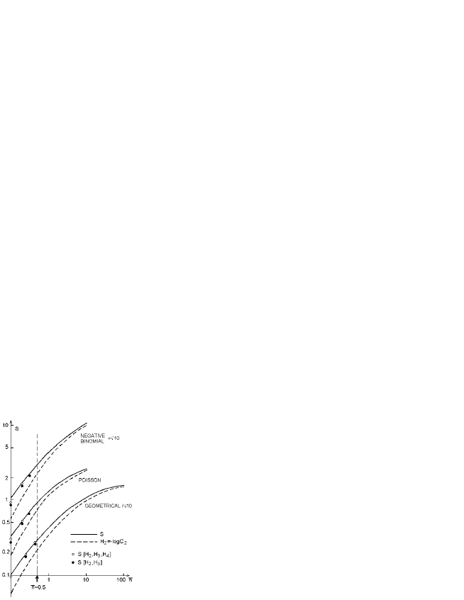
FIG. 1.: Estimates of entropy for systems with commonly encountered distributions using the extrapolation given by Eq.(22), plotted versus average multiplicity. Continuous lines: entropy calculated directly from (7). Dashed lines: entropy calculated from (5). Open points: Three-term extrapolation (24). Full points: Two-term extrapolation (23).

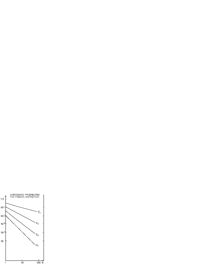
FIG. 2.: Coincidence probabilities for Poisson distribution versus average multiplicity.

REFERENCES

- [1] See e.g. Proceedings of XIII Int. Conf. on Ultrarelativistic Nucleus-Nucleus Collisions, Dec 1-5, 1997, Tsukuba, Nucl. Phys. A 638 (1998).
- [2] A.C. Gutzwiller, Chaos in Classical and Quantum Mechanics, Springer Verlag (1990), Chapter 10.
- [3] P.A. Miller, S. Sarkar and R. Zarum, Acta Phys. Pol. B 29, 3646 (1998).
- [4] See e.g. F. Becattini, Z. Phys. C 69, 485 (1996); J.Rafelski, J. Letessier and A. Tounsi, Acta Phys. Pol. B 27, 1037 (1996); M.Ga dzicki and M.I. Gorenstein, Acta Phys. Pol. B 30, no 9 (1999), to be published; F.Beccatini and U. Heinz, Z. Phys. C 76, 269 (1997); K.Geiger, Phys. Rev. D 46, 4986 (1992).
- [5] A. Bialas, W. Czyz and J. Wosiek, Acta Phys. Pol. B 30, 107 (1999).
- [6] S.K. Ma, Statistical Mechanics, World Scientific (1985), p.425. S.K. Ma, J. Stat. Phys. 26, 221 (1981). S.K. Ma and M. Payne, Phys. Rev. B 24, 3984 (1981).
- [7] V. Simak, M. Sumbera and I. Zborovski, Phys. Lett. B 206, 159 (1988).
- [8] E. Fermi, Prog. Theor. Phys. 5, 570 (1950); Elementary Particles, New Haven: Yale Univ. Press, 1951, Section 26.
- [9] C.E. Shannon, Bell system Tech. J. 27, 379, 623 (1948).
- [10] S.F. Edwards and P.W. Anderson, J. Phys. F 5, 965 (1975); G.Parisi, Phys. Rev. Lett. 43, 1754 (1979).
- [11] A. Renyi, Berkeley Symp. Prob. Stat. 1, 547 (1961).
- [12] A. Bialas and R. Peschanski, Nucl. Phys. B 273, 703 (1986).
- [13] Z. Cao and R.C. Hwa, Phys. Rev. Lett. 75, 1268 (1995); Phys. Rev. D 53, 6608 (1996); R. Hwa, Acta Phys. Pol. B 27, 1789 (1996).