Neutrino Mixing in the Seesaw Model

1 Introduction

Since the observation of neutrino oscillations,[1, 2, 3] the mixing matrix of the lepton sector (the MNS matrix [4]) has been discussed in many works. Among the various proposed explanations of the light neutrino mass, the seesaw mechanism [5] is an attractive scenario. In this paper, we study the MNS matrix in the framework of the seesaw model. Specifically, we assume that the gauge group is $SU(2)\times U(1)$. Since there are three light neutrinos, each one may have its partner, a gauge singlet neutrino with large Majorana mass. Moreover, neutrino oscillation experiments [1, 2, 3] suggest that there is mass hierarchy. In the context of the seesaw model, the mass hierarchy may originate from the Yukawa term and/or Majorana mass term. To account for the hierarchy and the mixing, there are two extreme explanations. The first explanation is that the hierarchy comes from the Majorana mass term. The other explanation is that the heavy right-handed neutrinos have a degenerate mass and the hierarchy comes from the Yukawa term. In this paper, we are interested in the former case. If the mass hierarchy of neutrinos comes from the hierarchy of the Majorana mass term $(m_{N1}\gg m_{N2}\gg m_{N3})$, the diagonalization of the seesaw matrix is carried out in a very different way than that for charged fermions. This is what we discuss in this paper. The seesaw mass matrix is a $2N_{f}\times 2N_{f}$ matrix ($N_{f}=3$ in our case) and has the simple structure

$$M_{\nu}=\left(\begin{array}[]{cc}0&y_{\nu}\frac{v}{\sqrt{2}}\\ {{y_{\nu}}^{T}}\frac{v}{\sqrt{2}}&m_{N}\\ \end{array}\right).$$ (3)

Its $N_{f}\times N_{f}$ submatrix corresponding to the Majorana mass term of light neutrinos is zero, and the submatrix corresponding to the Majorana mass term of heavy neutrinos can be a real diagonal matrix. The origin of the flavor mixing is the Dirac-type Yukawa term denoted by $y_{\nu}\frac{v}{\sqrt{2}}$. Because the seesaw matrix is a symmetric matrix, it can be diagonalized by a unitary matrix $V$ as $V^{T}M_{\nu}V$.[6] Despite the simple structure, it is not possible to diagonalize the matrix analytically, because we have to treat a $6\times 6$ matrix. We perform the approximate diagonalization of the mass matrix and obtain the parametrization of $V$. This produces the mixing matrix of neutrino sector. Combining it with the mixing matrix of the charged lepton sector, we may determine the flavor mixing in the lepton sector, namely, the MNS matrix. The method we employ is very similar to the diagonalization of the seesaw matrix for the quark mass in the context of a left-right model.[7] In the model, isosinglet quarks with a large mass hierarchy play a role similar to the right-handed heavy neutrino in the present case. An approximate diagonalization procedure of the seesaw type matrix is developed in Ref. 8). In this paper, we extend that method to the seesaw model for the neutrino mass with the same gauge group and higgs as in the standard model.

The paper is organized as follows. In section 2, by demonstrating the procedure of the diagonalization in the basis in which the Majorana mass term is diagonalized, we explain how the MNS matrix comes out by introducing a triangular matrix. In section 3, we study the special case that the Yukawa matrices for charged leptons and for neutrinos are simultaneously diagonalized through a biunitary transformation. If this were the case for the two Yukawa matrices of up- and down-type quarks, the Kobayashi-Maskawa (KM) matrix would be trivial. However, in the seesaw model for the neutrino mass, large mixing may still occur. We also discuss the phenomenological implications of our analysis. In section 4, we study the large mixing situation in the weak basis in which the Yukawa matrices of charged leptons and neutrinos are diagonal. In this basis, we study the texture of the Majorana mass matrix, which leads to the large mixing, and by doing so, we can understand the origin of the large mixing from a different angle. Finally, our conclusions are presented in section 5.

2 The MNS matrix in the Seesaw model

We start with the mass terms for lepton sector. Without loss of generality, the Majorana mass matrix $m_{N}$ is assumed to be a real diagonal matrix, ${m_{N}}_{ij}={m_{N}}_{i}\delta_{ij}$.[6] Writing $M_{\nu}$ in Eq. (3) in the diagonal Majorana mass basis, the mass terms are

$$-{\cal L}_{lepton} = \overline{e_{L}^{0}}y_{e}\frac{v}{\sqrt{2}}e_{R}^{0}$$ (10)

$$+ (\overline{{\nu_{L}^{0}}}~{}~{}\overline{{N_{R}^{0}}^{c}})\left(\begin{array}[]{cccccc}0&0&0&&&\\ 0&0&0&&y_{\nu}\frac{v}{\sqrt{2}}&\\ 0&0&0&&&\\ &&&m_{N1}&&\\ &{y_{\nu}}^{T}\frac{v}{\sqrt{2}}&&&m_{N2}&\\ &&&&&m_{N3}\\ \end{array}\right){{\nu_{L}^{0}}^{c}\choose N_{R}^{0}}+h.c.$$

We focus on the case that the Majorana mass term is much larger than Dirac mass term: $m_{N}\gg y_{\nu}\frac{v}{\sqrt{2}}$. We are interested in the case that the diagonal Majorana masses satisfy the relations ${m_{N}}_{i}\gg{m_{N}}_{j}$ ($i<j$), and the rank of the Yukawa matrices $y_{e}$ and $y_{\nu}$ is $N_{f}$.

The approximate diagonalization procedure of the seesaw-type matrix goes as follows. $M_{\nu}$ is diagonalized by a $2N_{f}\times 2N_{f}$ unitary matrix as $V^{T}M_{\nu}V={M_{\nu}}_{\rm diagonal}$. Let us parametrize this unitary matrix as[9]

$$V=\left(\begin{array}[]{cc}S&K\\ T&A\\ \end{array}\right),$$ (14)

where $S,K,T$ and $A$ are $N_{f}\times N_{f}$ submatrices. The unitarity relation is written in terms of the submatrices:

$$SS^{\dagger}+KK^{\dagger}=1,$$ (15)

$$TT^{\dagger}+AA^{\dagger}=1,$$ (16)

$$ST^{\dagger}+KA^{\dagger}=0.$$ (17)

Then ${M_{\nu}}_{\rm diagonal}$ is given by

$${M_{\nu}}_{\rm diagonal}=V^{T}M_{\nu}V=$$

$$\left(\begin{array}[]{cc}T^{T}{{y_{\nu}}^{T}}\frac{v}{\sqrt{2}}S+S^{T}y_{\nu}\frac{v}{\sqrt{2}}T+T^{T}m_{N}T&T^{T}{{y_{\nu}}^{T}}\frac{v}{\sqrt{2}}K+S^{T}y_{\nu}\frac{v}{\sqrt{2}}A+T^{T}m_{N}A\\ (T^{T}{{y_{\nu}}^{T}}\frac{v}{\sqrt{2}}K+S^{T}y_{\nu}\frac{v}{\sqrt{2}}A+T^{T}m_{N}A)^{T}&A^{T}{{y_{\nu}}^{T}}\frac{v}{\sqrt{2}}K+K^{T}y_{\nu}\frac{v}{\sqrt{2}}A+A^{T}m_{N}A\\ \end{array}\right).$$ (20)

We can easily see that the submatrices

$$T^{T}{{y_{\nu}}^{T}}\frac{v}{\sqrt{2}}S+S^{T}y_{\nu}\frac{v}{\sqrt{2}}T+T^{T}m_{N}T,$$ (22)

$$A^{T}{{y_{\nu}}^{T}}\frac{v}{\sqrt{2}}K+K^{T}y_{\nu}\frac{v}{\sqrt{2}}A+A^{T}m_{N}A$$ (23)

must be diagonal, and the off-diagonal submatrix becomes zero:

$$T^{T}{{y_{\nu}}^{T}}\frac{v}{\sqrt{2}}K+S^{T}y_{\nu}\frac{v}{\sqrt{2}}A+T^{T}m_{N}A=0.$$ (24)

In order for the $O(m_{N})$ part of Eq. (23) to be diagonal, we must have $A=1$ , because $m_{N}$ is diagonal and its diagonal elements are not degenerate. Then Eq. (16) implies that the leading order of $T$ is O($\frac{v}{m_{N}}$). Equation (17) means $K=O(\frac{v}{m_{N}})S$. Therefore, to leading order, $S^{\dagger}S=1$. In order for the $O(v)$ contribution of the RHS of Eq. (24) to be canceled, we can neglect the contribution of the first term. Then the relation $T=-\frac{v}{\sqrt{2}m_{N}}y_{\nu}^{T}S$ is obtained. $K$ is also determined through Eq. (17). The above consideration leads to the following submatrices:

$$A=1-O\left(\frac{v}{{m_{N}}}\right),\quad S{S}^{\dagger}=1-O\left(\frac{v^{2}}{{m_{N}}^{2}}\right),\quad T=-\frac{v}{\sqrt{2}m_{N}}y_{\nu}^{T}S,\quad K={y_{\nu}}^{*}\frac{v}{\sqrt{2}m_{N}}.$$

Below, we neglect the deviation from unity of $A$ and $SS^{\dagger}$. Now, the seesaw mass matrix is written as

$$V^{T}{M_{\nu}}V=\left(\begin{array}[]{cc}-S^{T}{y_{\nu}}\frac{v^{2}}{2m_{N}}{y_{\nu}}^{T}S&0\\ 0&m_{N}+O(v)\\ \end{array}\right).$$ (28)

At this stage, the unitary matrix is parametrized as

$$V=\left(\begin{array}[]{cc}1&{y_{\nu}}^{*}\frac{v}{\sqrt{2}m_{N}}\\ -\frac{v}{\sqrt{2}m_{N}}y_{\nu}^{T}&1\\ \end{array}\right)\left(\begin{array}[]{cc}S&0\\ 0&1\\ \end{array}\right).$$ (33)

Further,$S$ must be chosen so that the $-S^{T}y_{\nu}\frac{v^{2}}{2m_{N}}y_{\nu}^{T}S$ is diagonal. For any matrix $y$ of rank $N_{f}$, we can find a unitary matrix which transforms $y$ into a triangular form.[8] We choose such matrix as $S^{T}$:

$$S^{T}y_{\nu}=\left(\begin{array}[]{ccc}y_{1}&0&0\\ y_{21}&y_{2}&0\\ y_{31}&y_{32}&y_{3}\\ \end{array}\right)\equiv y_{\triangle}.$$ (37)

Here the diagonal elements are real, and the off-diagonal elements are complex in general. In this form, it is noted that the lightest neutrino $\nu_{e}$ only interacts with $N_{1}$, $\nu_{\mu}$ couples to both $N_{1}$ and $N_{2}$, and $\nu_{\tau}$ couples to all heavy neutrinos $N_{1},~{}N_{2}$ and $N_{3}$, as shown in Fig. 1. By choosing $S$ in this way, the seesaw mass matrix is approximately diagonalized. This is shown by writing submatrix $-S^{T}{y_{\nu}}\frac{1}{m_{N}}{y_{\nu}}^{T}S$:

$$-S^{T}{y_{\nu}}\frac{1}{m_{N}}{y_{\nu}}^{T}S=-\left(\begin{array}[]{ccc}\frac{{y_{1}}^{2}}{m_{N1}}&\frac{y_{1}y_{21}}{m_{N1}}&\frac{y_{1}y_{31}}{m_{N1}}\\ \frac{y_{1}y_{21}}{m_{N1}}&\frac{{y_{2}}^{2}}{m_{N2}}+\frac{{y_{21}}^{2}}{m_{N1}}&\frac{y_{21}y_{31}}{m_{N1}}+\frac{y_{2}y_{32}}{m_{N2}}\\ \frac{y_{1}y_{31}}{m_{N1}}&\frac{y_{21}y_{31}}{m_{N1}}+\frac{y_{2}y_{32}}{m_{N2}}&\frac{{y_{3}}^{2}}{m_{N3}}+\frac{{y_{32}}^{2}}{m_{N2}}+\frac{{y_{31}}^{2}}{m_{N1}}\\ \end{array}\right).$$ (41)

Because $m_{N1}\gg m_{N2}\gg m_{N3}$, the off-diagonal elements are much smaller than the difference of the diagonal elements. Therefore the mass matrix is regarded as approximately diagonal:

$$V^{T}M_{\nu}V\simeq\left(\begin{array}[]{cccccc}-\frac{{y_{1}}^{2}v^{2}}{2m_{N1}}&&&&&\\ &-\frac{{y_{2}}^{2}v^{2}}{2m_{N2}}&&&&\\ &&-\frac{{y_{3}}^{2}v^{2}}{2m_{N3}}&&&\\ &&&m_{N1}&&\\ &&&&m_{N2}&\\ &&&&&m_{N3}\\ \end{array}\right).$$ (48)

The above matrices show that the mass of $\nu_{e}$ is determined by the mass of the heaviest singlet neutrino, $N_{1}$, and is not affected by the presence of the other lighter singlet neutrinos, because $\nu_{e}$ couples to only $N_{1}$. Moreover, though $\nu_{\mu}$ couples to both $N_{1}$ and $N_{2}$, its mass is mainly determined by the mass of $N_{2}$, because the mass of $N_{1}$ is much larger than that of $N_{2}$. Similarly, the mass of the $N_{3}$ mainly depends on the mass of $N_{3}$, due to the relation $m_{N1}\gg m_{N2}\gg m_{N3}$. If such a mass hierarchy of the three heavy neutrinos is admitted, this procedure is a powerful method for diagonalizing the seesaw-type mass matrix.

Then, the unitary matrix $V$ can be rewritten as

$$V=\left(\begin{array}[]{cc}S&0\\ 0&1\\ \end{array}\right)\left(\begin{array}[]{cc}1&{y_{\triangle}}^{*}\frac{v}{\sqrt{2}m_{N}}\\ -\frac{v}{\sqrt{2}m_{N}}{y_{\triangle}}^{T}&1\\ \end{array}\right).$$ (53)

The MNS matrix is a $3\times 6$ submatrix of $V$ multiplied by a $3\times 3$ unitary matrix for diagonalization of the Yukawa term of the charged lepton,

$$V_{MNS}=({V_{Le}}^{\dagger}S^{*})(1,y_{\triangle}\frac{v}{\sqrt{2}m_{N}}).$$ (54)

Here $V_{Le}$ comes from the diagonalization of the Yukawa term of the charged lepton and is defined by the equations

$$e^{0}_{L}=V_{Le}e_{L},$$ (55)

$$e^{0}_{R}=V_{Re}e_{R},$$ (56)

$$y_{eD}={V_{Le}}^{\dagger}y_{e}{V_{Re}},$$ (57)

where $y_{eD}$ is a real diagonal matrix. We introduce a unitary matrix which transforms the Yukawa term of neutrinos $y_{\nu}$ to the diagonal form $y_{\nu D}$:

$$y_{\nu} = V_{L\nu}y_{\nu D}{V_{R\nu}}^{\dagger}$$ (58)

$$= S^{*}y_{\triangle}.$$

The second line of Eq. (58) comes from Eq. (37). Therefore we can relate $y_{\triangle}$ and $y_{\nu D}$ through the equation

$$y_{\nu D} = {V_{L\nu}}^{\dagger}S^{*}y_{\triangle}V_{R\nu}$$ (59)

$$= S^{\prime*}y_{\triangle}V_{R\nu},$$

where we introduce another unitary matrix $S^{\prime}$,

$${S^{\prime}}^{*}={V_{L\nu}}^{\dagger}S^{*}.$$ (60)

$S^{\prime}$ represents the difference between the unitary matrix which transforms $y_{\nu}$ into the triangular form and the unitary matrix for the diagonalization by a biunitary transformation.

Finally, we can write the leptonic charged current as

$$J_{L\mu} = (\bar{e}_{L}\bar{\mu}_{L}\bar{\tau}_{L})\gamma_{\mu}V_{MNS}\left(\begin{array}[]{c}{\nu_{L1}}\\ {\nu_{L2}}\\ {\nu_{L3}}\\ {N_{R1}}^{c}\\ {N_{R2}}^{c}\\ {N_{R3}}^{c}\\ \end{array}\right),$$ (67)

with

$$V_{MNS} = ({V_{Le}}^{\dagger}S^{*})(1,y_{\triangle}\frac{v}{\sqrt{2}m_{N}})$$ (68)

$$= (V_{KM}S^{\prime*})(1,y_{\triangle}\frac{v}{\sqrt{2}m_{N}}),$$

and

$$V_{KM}={V_{Le}}^{\dagger}V_{L\nu}.$$ (69)

Here $\nu_{L}$ and ${N_{R}}^{c}$ are mass eigenstates of neutrinos. From the first definition of $V_{MNS}$ from Eq. (67), we can see that the mixing of the neutrino sector is determined by the unitary matrix which transforms the neutrino Yukawa term into the triangular form. In the second definition of $V_{MNS}$ from Eq. (67), we introduce the usual KM-like matrix and rewrite the matrix ${V_{Le}}^{\dagger}S^{*}$ as $({V_{Le}}^{\dagger}V_{L\nu})({V_{L\nu}}^{\dagger}S^{*})=V_{KM}S^{\prime*}$. By rewriting the matrix in this way, we can divide the lepton mixing angles into two parts, one which comes from the usual KM-like part, denoted by $V_{KM}$, and another ($S^{\prime}$) which comes from the difference between the unitary matrix $V_{L\nu}$ for biunitary transformation and the unitary matrix $S$ for transformation into the triangular form. The advantage of the latter decomposition is that both $V_{KM}$ and $S^{\prime}$ are independent of the choice of the weak basis.

We now summarize the results obtained in this section. The MNS matrix is a product of the mixing matrix of the charged lepton sector and that of the neutrino sector. We find that the unitary matrix denoted by ${V_{Le}}^{\dagger}S^{*}$ determines the mixing matrix among light leptons. Here $S$ denotes the unitary matrix which transforms the neutrino Yukawa term into a triangular matrix. $V_{Le}$ is the unitary matrix for the diagonalization of the charged lepton Yukawa term. This is proved in the weak basis in which Majorana mass matrix of heavy neutrinos is real diagonal and also under the assumption that the heavy Majorana neutrinos have greatly differing mass scales.

3 Large mixing

The MNS matrix obtained in the previous section is divided into two parts unitary matrices $S^{\prime}$ and $V_{KM}$. We note that $S^{\prime}$ is determined by $y_{\nu}$ and $m_{N}$ in the diagonal Majorana basis, while $V_{KM}$ is determined by $y_{\nu}{y_{\nu}}^{\dagger}$ and $y_{e}{y_{e}}^{\dagger}$. Therefore $S^{\prime}$ is determined by the mass matrix of the neutrino sector, while $V_{KM}$ is determined by the Yukawa terms only. In order for $V_{KM}$ to be a non-trivial matrix, the following condition must be satisfied:

$$V_{KM}\neq 1\quad\leftrightarrow\quad[y_{e}{y_{e}}^{\dagger},y_{\nu}{y_{\nu}}^{\dagger}]\neq 0.$$ (70)

On the other hand, the condition for $S^{\prime}$ being non-trivial is

$$S^{\prime}\neq 1\quad\leftrightarrow\quad(y_{\triangle}{y_{\triangle}}^{\dagger})_{ij}\neq 0\quad{\rm for}\quad(i\neq j),$$ (71)

in the diagonal Majorana basis. Equation (71) comes from Eq. (59), because

$${S^{\prime}}^{*}{y_{\triangle}}{y_{\triangle}}^{\dagger}{S^{\prime}}^{T}={y_{\nu D}}^{2}.$$ (72)

The mixing angle is the product of $S^{\prime}$ and $V_{KM}$. We note that for a given $y_{\triangle}$ we may determine $S^{\prime}$. Equation (71) and (72) imply that the off-diagonal elements in the triangular matrix $y_{\triangle}$ induce the mixing in $S^{\prime}$. If the off-diagonal elements of $y_{\triangle}$ vanish, $S^{\prime}=1$. However, since $V_{KM}$ is arbitrary, in general, lepton mixing angles are also arbitrary. Even if there is large mixing in $S^{\prime}$, this can be canceled by $V_{KM}$. There may also be the case that $S^{\prime}$ is the unit matrix and there is large mixing in $V_{KM}$. Here we focus on the case that $V_{KM}=1$. Equivalently, we impose the commutation relation

$$[y_{e}{y_{e}}^{\dagger},y_{\nu}{y_{\nu}}^{\dagger}]=0.$$ (73)

If this is the case, $S^{\prime}$ determines the mixing angles.

Now we show that large mixing occurs without fine tuning of the matrix elements of $y_{\triangle}$. We illustrate this by considering the two flavor case $(N_{f}=2)$ and apply Eq. (73) to the explanation of the large mixing of atmospheric neutrinos. In the two flavor case, $y_{\triangle}y_{\triangle}^{\dagger}$, $S^{\prime}$ and the approximately diagonalized light neutrino mass matrix $m_{\nu}$ are respectively expressed as

$$y_{\triangle}y_{\triangle}^{{\dagger}}=\left(\begin{array}[]{cc}{y}_{2}^{2}&{y}_{2}{y}_{32}^{*}\\ {y}_{2}{y}_{32}&|{y}_{32}|^{2}+{y}_{3}^{2}\end{array}\right),$$ (76)

$$S^{\prime}=\left(\begin{array}[]{cc}\cos\theta&-\sin\theta e^{i\phi}\\ \sin\theta e^{-i\phi}&\cos\theta\end{array}\right),$$ (79)

with

$$\tan 2\theta=\frac{2|{y}_{32}|{y}_{2}}{-{y}_{2}^{2}+|{y}_{32}|^{2}+{y}_{3}^{2}},\quad\phi=\arg({y}_{32}),$$ (80)

and

$$m_{\nu}=-\left(\begin{array}[]{cc}\frac{{y_{2}}^{2}}{m_{N2}}&\frac{y_{2}y_{32}}{m_{N2}}\\ \frac{y_{2}y_{32}}{m_{N2}}&\frac{{y_{3}}^{2}}{m_{N3}}+\frac{{y_{32}}^{2}}{m_{N2}}\\ \end{array}\right)\frac{v^{2}}{2},$$ (83)

where $m_{N2}\gg m_{N3}$ is assumed. In order that Eq. (83) can be regarded as an approximately diagonal matrix, the sufficient conditions on the elements of the Yukawa term $y_{\triangle}$ are

$${\cal O}(y_{2})={\cal O}(y_{3})\equiv y,$$ (84)

$${\cal O}\left(\frac{|y_{32}|}{y}\right)\leq 1.$$ (85)

The first condition is that the hierarchy of the light neutrino masses comes from the hierarchy of the Majorana mass term, $m_{N2}\gg m_{N3}$. The second condition suppresses further mixing from the form of Eq. (83).

In Fig. 2, we show $\sin^{2}2\theta$ as a function of $\frac{|y_{32}|}{y_{2}}$ by changing the ratio $r={\frac{y_{3}}{y_{2}}}$. For $r=1$, maximal mixing occurs at infinitesimally small $|y_{32}|=\epsilon$, and the mixing decreases as $|y_{32}|$ increases. For $r<1$, maximal mixing occurs at non-zero $y_{32}$ because the diagonal elements are degenerate for $|y_{32}|\neq 0$. For $r>1$, the mixing angle is suppressed because the diagonal elements cannot be degenerate. For $r\neq 1$, small mixing is also possible for $|y_{32}|\ll|y_{3}-y_{2}|$. In Fig. 3, we constrain the ratios of the Yukawa couplings by using the result obtained by the Super-Kamiokande, Eq. (91). The allowed range is between two curves in the parameter space, $(r,\frac{|y_{32}|}{y_{2}})$. We can see that the experimental constraint can be easily satisfied for the range of the parameters in Eqs. (84) and (85). The curves are obtained with the equation

$$\biggr{(}\frac{{y}_{3}}{{y}_{2}}\biggr{)}^{2}+\biggr{(}\frac{|{y}_{32}|}{{y}_{2}}-\frac{1}{\tan 2\theta}\biggr{)}^{2}=1+\frac{1}{\tan^{2}2\theta},$$ (86)

where $\sin^{2}2\theta$ takes the minimum and the maximum values of the experimental constraint, Eq. (91). The qualitative features of Figs. 2 and 3 can be understood by using the approximate formulae for $\tan 2\theta$ under the conditions set by Eq. (84) and Eq. (85). From Eq. (80) we have

$$\tan 2\theta=\left\{\displaystyle\begin{array}[]{lc}\frac{2y}{|y_{32}|}\geq 2&\mbox{for}\quad|y_{32}|^{2}>y_{3}^{2}-y_{2}^{2},\\ \frac{|{y}_{32}|}{y_{3}-y_{2}}&\mbox{for}\quad|y_{32}|^{2}<y_{3}^{2}-y_{2}^{2}.\end{array}\right.$$ (89)

The first line corresponds to the case that the diagonal elements are very degenerate and the second line to the case that they are not degenerate. The first case of Eq. (89) leads to

$$\sin^{2}2\theta\geq 0.8.$$ (90)

This can be compared with the result for atmospheric neutrinos. The Super-Kamiokande collaboration [3] has reported the range

$$\sin^{2}2\theta_{\rm atm}\geq 0.8.$$ (91)

Moreover, the second line in Eq. (89) means that large mixing occurs for $|y_{32}|\sim|y_{3}-y_{2}|$.

Finally, we comment on the mass scale $m_{N3}$ of the lightest gauge singlet neutrino. According to the Super-Kamiokande result, the mass-squared difference of the $\mu$ and $\tau$ neutrinos is of order $10^{-3}{\rm[eV^{2}]}$. Assuming that this corresponds to the mass squared of the $\tau$ neutrino and that the Yukawa coupling is the same order of magnitude as the gauge coupling, we obtain

$$m_{\nu\tau}\simeq\frac{{M_{W}}^{2}}{m_{N3}}.$$ (92)

Therefore, the mass of the lightest gauge singlet neutrino may be ${\cal O}(10^{14})$ [GeV].

4 Texture of the Majorana mass

In the previous section, we obtained large mixing under the additional constraint that the Yukawa matrices of charged leptons, $y_{e}y_{e}^{\dagger}$, and neutrinos, $y_{\nu}y_{\nu}^{\dagger}$, are simultaneously diagonalized, i.e. $V_{Le}=V_{L\nu}$ [see Eq. (73)]. The origin of the mixing may be traced to the presence of the off-diagonal element of the triangular matrix in the diagonal Majorana mass basis. It is useful to study the same situation from a different viewpoint. In this section, we study the large mixing case in a different basis. We can transform from the diagonal Majorana mass basis to the diagonal basis of Yukawa terms for charged leptons and neutrinos. If we further impose the condition Eq. (73), the transformation becomes a transformation of the weak basis. Therefore $V_{MNS}$ becomes the $3\times 3$ unit matrix. In the new basis, the Majorana mass term is not diagonal, and we may investigate the texture of the Majorana matrix that induces large mixing.

In this basis, the mass term (LABEL:L1) is rewritten as

$$-{\cal L}_{lepton}=\overline{e}_{L}{y_{eD}}\frac{v}{\sqrt{2}}e_{R}+(\overline{\nu^{\prime}_{L}}~{}~{}\overline{{N^{\prime}_{R}}^{c}})\left(\begin{array}[]{cc}0&y_{\nu D}\frac{v}{\sqrt{2}}\\ y_{\nu D}\frac{v}{\sqrt{2}}&{V_{R\nu}}^{T}m_{N}V_{R\nu}\end{array}\right){{\nu^{\prime}_{L}}^{c}\choose N^{\prime}_{R}}+h.c.,$$ (95)

(96)

where

$$\nu^{\prime}_{L}={V_{L\nu}}^{\dagger}\nu_{L}^{0},$$ (97)

$$N^{\prime}_{R}={V_{R\nu}}^{\dagger}N^{0}_{R},$$ (98)

and the leptonic charged current is

$$J_{L\mu} = (\bar{e}_{L}\bar{\mu}_{L}\bar{\tau}_{L})V_{KM}\gamma_{\mu}\left(\begin{array}[]{c}{\nu_{L1}^{\prime}}\\ {\nu_{L2}^{\prime}}\\ {\nu_{L3}^{\prime}}\end{array}\right).$$ (102)

Up to this point, we have not imposed the condition Eq. (73). If this condition is imposed, namely $V_{KM}=1$, the charged current becomes

$$J_{L\mu}=(\bar{e}_{L}\bar{\mu}_{L}\bar{\tau}_{L})\gamma_{\mu}\left(\begin{array}[]{c}{\nu_{L1}^{\prime}}\\ {\nu_{L2}^{\prime}}\\ {\nu_{L3}^{\prime}}\end{array}\right).$$ (106)

${V_{R\nu}}^{T}m_{N}V_{R\nu}$ $(\equiv\tilde{m}_{N})$ is the Majorana mass matrix in the basis of the diagonal Yukawa term. Because of Eq. (59), $V_{R\nu}$ is determined by ${y_{\triangle}}^{\dagger}y_{\triangle}$ as

$${y_{\nu D}}^{2}={V_{R\nu}}^{\dagger}{y_{\triangle}}^{\dagger}y_{\triangle}V_{R\nu}.$$ (107)

Now we give the form of the Majorana mass matrix that induces large mixing in the two flavor case $(N_{f}=2)$. Because ${y_{\triangle}}^{\dagger}y_{\triangle}$ is expressed as

$${y_{\triangle}}^{\dagger}y_{\triangle}=\left(\begin{array}[]{cc}{y_{2}}^{2}+|y_{32}|^{2}&{y_{32}}^{*}y_{3}\\ y_{32}y_{3}&{y_{3}}^{2}\end{array}\right),$$ (110)

we can parametrize $V_{R\nu}$ as

$$V_{R\nu}=\left(\begin{array}[]{cc}\cos\alpha&-\sin\alpha~{}e^{i\beta}\\ \sin\alpha~{}e^{-i\beta}&\cos\alpha\end{array}\right),$$ (113)

with

$$\tan 2\alpha=\frac{2|y_{32}|y_{3}}{{y_{2}}^{2}+|y_{32}|^{2}-{y_{3}}^{2}},\quad\beta=-{\rm arg}(y_{32}).$$ (114)

Therefore, the Majorana mass matrix is written as

$$\tilde{m}_{N}=\left(\begin{array}[]{cc}m_{N2}\cos^{2}\alpha+m_{N3}\sin^{2}\alpha~{}e^{-2i\beta}&-\frac{1}{2}(m_{N2}e^{i\beta}-m_{N3}e^{-i\beta})\sin 2\alpha\\ -\frac{1}{2}(m_{N2}e^{i\beta}-m_{N3}e^{-i\beta})\sin 2\alpha&m_{N2}\sin^{2}\alpha~{}e^{2i\beta}+m_{N3}\cos^{2}\alpha\end{array}\right).$$ (117)

In Fig. 4, we display the $\sin^{2}2\alpha$ as a function $\frac{|y_{32}|}{y_{2}}$ by changing the ratio $r={\frac{y_{3}}{y_{2}}}$. By comparing Figs. 3 and 4, we can see that maximal mixing of the mixing angle $\theta$ and maximal mixing of $\alpha$ take place at the same time only when the diagonal elements of $y_{\triangle}$ are exactly degenerate ($r=1$). In this case, by setting $\sin^{2}2\alpha\sim 1$, the Majorana mass matrix can be expressed as

$$\tilde{m}_{N}\simeq\frac{m_{N2}}{2}\left(\begin{array}[]{cc}1+\epsilon e^{-2i\beta}&-(1-\epsilon e^{-2i\beta})e^{i\beta}\\ -(1-\epsilon e^{-2i\beta})e^{i\beta}&(1+\epsilon e^{-2i\beta})e^{2i\beta}\end{array}\right),$$ (121)

where $\epsilon=m_{N3}/m_{N2}$ $(\ll 1)$. From Eq. (121), the texture which leads to large mixing has the characteristic feature that the off-diagonal and diagonal elements are the same order of magnitude and the Majorana mass matrix is close to a democratic-type matrix. There are small corrections to the democratic-type matrix, which lead to the non-zero mass of the heavy neutrino $N_{3}$.

5 Conclusions and discussion

We have studied the MNS matrix in the seesaw model. We proposed an approximate procedure for diagonalization of the seesaw matrix. If we start with a real diagonal Majorana mass matrix and assume a hierarchy for the masses of the heavy neutrinos, we find that the unitary matrix $S$ that transforms the Yukawa term into a triangular form determines the mass eigenstate of light neutrinos up to a small mixing of the heavy neutrinos. The triangular form has to be arranged in such a way that the lighter $SU(2)$ doublet neutrinos couple to the heavier singlet neutrinos. The mixing matrix for light leptons is $V_{Le}^{\dagger}S^{*}$, i.e., the product of the unitary matrix $V_{Le}$ required by diagonalization of the Yukawa matrices of charged leptons, $y_{e}y_{e}^{\dagger}$, and the unitary matrix $S^{*}$ to transform the Yukawa matrix of neutrinos, $y_{\nu}$, into the triangular form $y_{\triangle}$. By inserting the unitary matrix for the diagonalization of the Yukawa matrices of the neutrinos $y_{\nu}y_{\nu}^{\dagger}$, the mixing matrix can be rewritten as $V_{KM}{S^{\prime}}^{*}$. $V_{KM}$ is a usual KM-like matrix and denotes the difference between the unitary matrices for the diagonalization of Yukawa terms, and $S^{\prime}$ denotes the difference between the unitary matrix for the transformation into the triangular form and the unitary matrix for the diagonalization of $y_{\nu}$. Therefore $S^{\prime}$ can be determined by the structure of the mass matrix of the neutrino sector only. We find that for a given $y_{\triangle}$, we can determine $S^{\prime}$. We also find that the presence of the off-diagonal element of $y_{\triangle}$ induces the mixing in $S^{\prime}$. A large mixing angle is possible and it was explicitly given for the two-flavor case. Since $V_{KM}$ is arbitrary, we impose the additional condition Eq. (73) so that $S^{\prime}$ determines the mixing matrix. By doing so, we compare the obtained mixing angle with the atmospheric neutrino anomaly, which was reported by the Super-Kamiokande collaboration. Because the mixing angle is a function of the elements of $y_{\triangle}$, we can find the region of the elements which is compatible with the Super-Kamiokande results. We would like to comment that the origin of the commutation relation of the Yukawa terms may be the unification of the quark and lepton. Because the KM matrix is close to the unit matrix, this may suggest that up and down quark Yukawa terms may approximately satisfy similar commutation relations. Such a relation may also hold for the lepton sector in unified theories of quarks and leptons. The phenomenological study of such systems can be extended to the three flavor case and may be applied to the solar neutrino problem. We also note that Smirnov [10] studied mixing in the seesaw model. Because our approach differs from his, and the transformation to the triangular form is essential in our approach, the relation between our work and his must be carefully examined. We will study these issues in future publications.

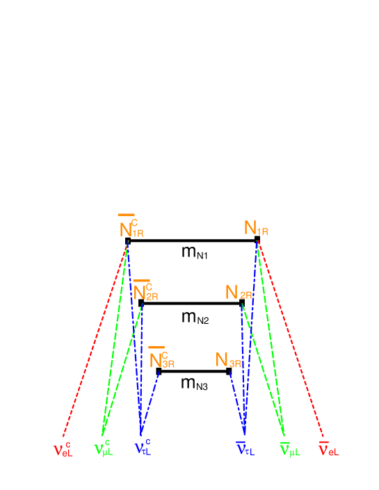
Fig. 1: In the form of $y_{\triangle}$, $\nu_{e}$ only couples to $N_{1}$, while $\nu_{\mu}$ couples to both $N_{1}$ and $N_{2}$, and $\nu_{\tau}$ couples to all heavy neutrinos, $N_{1}$, $N_{2}$ and $N_{3}$. The mass of $\nu_{e}$ depends only on $m_{N1}$. Moreover, due to the mass hierarchy $m_{N1}\gg m_{N2}\gg m_{N3}$, $\nu_{\mu}$ and $\nu_{\tau}$ are determined by the masses of $m_{N2}$ and $m_{N3}$, respectively.

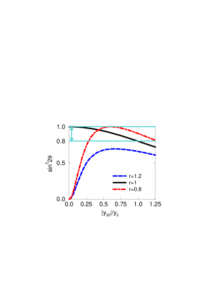
Fig. 2: $\sin^{2}2\theta$ as a function of ${|y_{32}|\over y_{2}}$ for various $r={y_{3}\over y_{2}}$. The three curves correspond to $r=1$ (solid line), $r=1.2$ (dotted line), and $r=0.8$ (dot-dashed line). The region between the two solid straight lines is allowed by the Super-Kamiokande experiment on atmospheric neutrinos, $0.8\leq\sin^{2}2\theta_{\rm atm}\leq 1$.

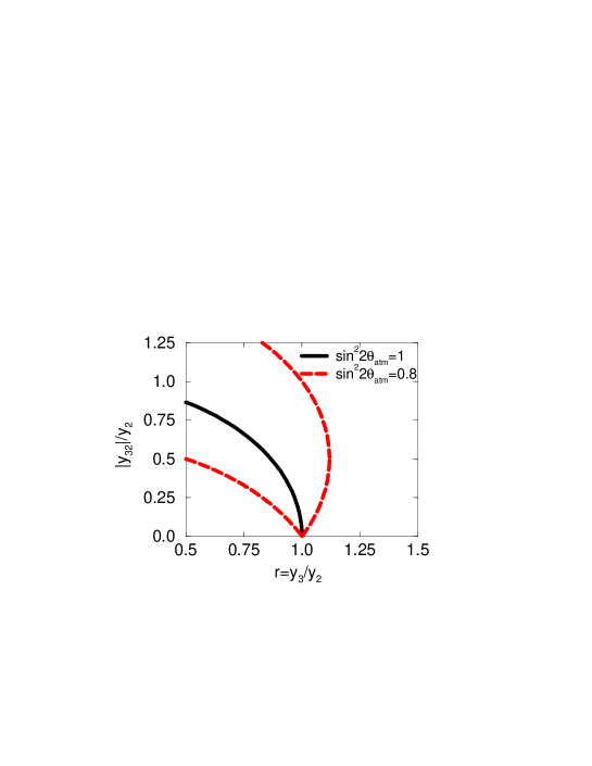
Fig. 3: The region in the parameter space $(\frac{y_{3}}{y_{2}},\frac{|y_{32}|}{y_{2}})$ between the dashed lines is allowed from the Super-Kamiokande experiment on atmospheric neutrinos, $\sin^{2}2\theta_{\rm atm}\geq 0.8$.

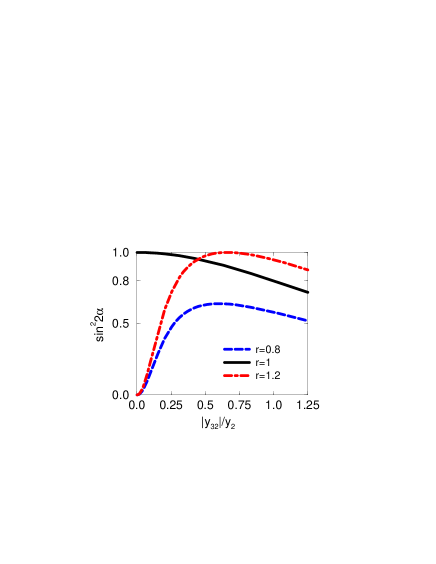
Fig. 4: $\sin^{2}2\alpha$ as a function of ${|y_{32}|\over y_{2}}$ for various $r={y_{3}\over y_{2}}$. The three curves correspond to $r=1$ (solid line), $r=1.2$ (dotted line), and $r=0.8$ (dot-dashed line).

References

-
[1]
K.S. Hirata et al., Phys. Rev. Lett. 65 (1990)
1297; Phys. Rev. Lett. 65 (1990) 1301;
Phys. Rev. D44 (1991) 2241;
D45, (1992) 2170(E).
Super-Kamiokande Coll., Y. Fukuda et al., Phys. Rev. Lett. 77 (1996) 1683; Phys. Rev. Lett. 81 (1998) 1158.
J. N. Abdurashitov et al., Phys. Lett. B328 (1994) 234.
GALLEX Coll., P. Anselmann et al., Phys. Lett. B327 (1994) 377; Phys. Lett. B342 (1995) 440. -
[2]
Y. Fukuda et al., Phys. Lett. B335 (1994) 237.
R. Becker-Szendy et al., Nucl. Phys. B(Proc. Suppl.) 38 (1995) 331.
W. W. M. Allison et al., Phys. Lett. B391 (1997) 491.
MACRO Coll., M. Ambrosio et al., Phys. Lett. B434 (1998) 451. - [3] Super-Kamiokande Coll., Y. Fukuda et al., Phys. Lett. B433 (1998) 9; Phys. Lett. B436 (1998) 33; Phys. Rev. Lett. 81 (1998) 1562.
- [4] Z. Maki, M. Nakagawa and S. Sakata, Prog. Theor. Phys. 28 (1962) 870.
-
[5]
T. Yanagida,
in Proceedings of the Workshop on ”The Unified
Theory and the Baryon Number of the Universe”, Edited by
Osamu Sawada and Akio Sugamoto, KEK 13-14 Feb 1979
(KEK-79-18).
M. Gell-Mann, P. Ramond and R. Slansky in Sanibel Talk, CALT-68-709, Feb. 1979, and in ”Supergravity” (North Holland, Amsterdam 1979). - [6] S. M. Bilenky and S.T. Petcov, Rev. Mod. Phys. 59 (1987) 671.
-
[7]
Z. G. Berezhiani, Phys. Lett. 129B (1983) 99;
Phys. Lett. 150B (1985) 177.
D. Chang and R. N. Mohapatra, Phys. Rev. Lett. 58 (1987) 1600.
J. Rajpoot, Phys.Lett. B191 (1987) 122.
A. Davidson and K. C. Wali, Phys. Rev. Lett. 59 (1987) 393.
K. S. Babu and R. N. Mohapatra, Phys. Rev. Lett. 62 (1989) 1079.
Y. Koide and H. Fusaoka, Z. Phys. C71 (1996) 459.
Y. Koide, hep-ph/9803458; Phys. Rev. D56 (1997) 2656. -
[8]
T. Morozumi, T. Satou, M. N. Rebelo and M. Tanimoto,
Phys. Lett. B410 (1997) 233.
Y. Kiyo, T. Morozumi, P. Parada, M. N. Rebelo and M. Tanimoto, Prog. Theor. Phys. 101 (1999) 671. -
[9]
G. C. Branco and L. Lavoura, Nucl. Phys. B278 (1986) 738.
G. C. Branco, T. Morozumi, P. A. Parada and M. N. Rebelo, Phys. Rev. D48 (1993) 1167. - [10] A. Yu. Smirnov, Phys. Rev. D48 (1993) 3264.