Gravitational production of gravitinos

Abstract

We calculate the number density of helicity $\pm 3/2$ gravitinos produced out of the vacuum by the non-static gravitational field in a generic inflation scenario. We compare it to the number density of gravitinos produced in particle interactions during reheating.

PACS numbers: 98.80.Cq

I Introduction

It was realized early on [1] that the gravitino could pose a serious cosmological problem in the context of a hot Big-Bang, if it were once in thermal equilibrium. An unstable gravitino, for instance, would decay in the post-Big-Bang nucleosynthesis era, if its mass $m_{3/2}\lesssim 10^{4}\,$GeV, and the entropy produced would ruin the successes of Big-Bang nucleosynthesis. Similarly, if the gravitino were stable, as e.g., in gauge mediated supersymmetry breaking, its energy density would eventually overclose the Universe, if its mass $m_{3/2}\gtrsim 2\,$keV. A solution to this problem was brought forward in Ref. [2]: if inflation took place, the gravitinos present at the time of Big-Bang nucleosynthesis were created during reheating, in an abundance possibly much smaller than that corresponding to thermal equilibrium. Cosmological constraints on their abundance could then be turned into useful upper limits on the reheating temperature $T_{\rm R}$ [3], typically $T_{\rm R}\lesssim 10^{8}-10^{10}\,$GeV, for an unstable gravitino with $m_{3/2}\lesssim 3\times 10^{3}\,$GeV, or $T_{\rm R}\lesssim 10^{2}-10^{10}\,$GeV, for a stable gravitino with $1\,{\rm keV}\lesssim m_{3/2}\lesssim 1\,{\rm GeV}$.

These studies assume that the gravitino abundance has been exponentially suppressed during inflation, and that gravitinos were only created in particle interactions during reheating. However, particles can be produced out of the vacuum in a non-static gravitational background if their coupling to the gravitational field is not conformal [4]. A well-known case is the production of gravitational waves or scalar density perturbations during inflation. As we argue below, a massive gravitino is not conformally invariant in a Friedmann–Robertson–Walker (FRW) background, and our main objective is thus to quantify the number density of gravitinos that can be produced gravitationally during inflation. We will consider a generic inflation scenario within $N=1$ supergravity [5], and briefly discuss the more particular case of pre-Big Bang cosmology [6]. The cosmological consequences of gravitino production during inflation were briefly discussed in Ref. [7]. These authors did not actually study the gravitational production of gravitinos, and rather focused on the spin 0 and spin 1/2 cases, as they were interested in the problem of moduli and modulini fields. With regards to the gravitino, they assumed that one particle would be produced per quantum state for modes with comoving wavenumber $k\lesssim H_{\rm I}$, where $H_{\rm I}$ denotes the Hubble scale of inflation. This estimate showed that gravitational production of gravitinos could pose a cosmological problem if the energy scale $V^{1/4}$ at which inflation takes place saturates its observational upper bound, i.e. $V^{1/4}\sim 10^{16}\,$GeV, and in this respect, it justifies further the present work. Our study is more specialized than that of Ref. [7], as we concentrate exclusively on the gravitino. However, it is also more systematic and more detailed, as we derive and solve the gravitino field equation to provide quantitative estimates of the number density of gravitinos produced. We also examine different cases for the magnitude and dynamics of the gravitino effective mass term during and after inflation. Finally, we also study the effect of a finite duration of the transition between inflation and reheating, using numerical integration of the field equation. This effect is important, as this timescale defines the “degree of adiabaticity” of the transition, and indeed the number density of gravitinos produced is found to be inversely proportional to it.

The study of the conformal behavior of the gravitino also bears interest of its own, apart from any application to cosmology, and to our knowledge, the quantization of quantum fields in curved space-time has been examined for spins 0, 1/2, 1 and 2, but not $3/2$ [4] (although the case of a massless gravitino in a perfect fluid cosmology was studied in Ref. [8]). In the present work, we focus on the helicity 3/2 modes of the gravitino. The field equations and the quantization of the helicity 1/2 modes are indeed more delicate, due to the presence of constraints. These constraints vanish identically if supersymmetry is unbroken [9]; in broken supersymmetry, these constraints do not vanish, but do not induce any inconsistency [10]. As shown below, these constraints apply to the modes of helicity 1/2, not to those of helicity 3/2, and for this reason, we leave the problem of the helicity 1/2 modes open for a further study; nonetheless, we present these field equations and their constraints. The number density of helicity 3/2 gravitinos produced during inflation that we derive in this paper should thus be interpreted as a lower limit. Quite probably, however, the number density of helicity 1/2 gravitinos should be of the same order as that of helicity 3/2, and the results correct within a factor of order 2.

This paper is organized as follows. In Section II, we derive the gravitino field equation for the $\pm 3/2$ helicity modes, and in Section III, we calculate the number density of gravitinos produced in a generic inflation scenario. We summarize our conclusions and briefly discuss the case of pre-Big-Bang string cosmology in Section IV. All throughout this paper, we use natural units $\hbar=c=m_{\rm Pl}=1$, where $m_{\rm Pl}\equiv(8\pi G)^{-1/2}$ is the reduced Planck mass. We note $M_{\rm Pl}\equiv\sqrt{8\pi}m_{\rm Pl}$ the Planck mass. Furthermore, we restrict ourselves to a FRW background, whose metric is written as: ${\rm d}s^{2}=g_{\mu\nu}{\rm d}x^{\mu}{\rm d}x^{\nu}=a^{2}(\eta)(-{\rm d}\eta^{2}+{\rm d}x^{2}+{\rm d}y^{2}+{\rm d}z^{2})$, where $a(\eta)$ is the scale factor, and $\eta$ denotes conformal time; the Minkowski metric is written $\eta_{ab}$. We also use standard conventions on the derivative of the Kähler potential $G(z_{i},z_{i}^{\ast})$ with respect to the scalar components $z_{i}$ of chiral superfields: $G^{i}\equiv\partial G/\partial z_{i}$, $G_{i^{\ast}}\equiv\partial G/\partial z^{i\ast}$. Other notations, relative to the Dirac matrices, are given in the Appendix.

II Field equation

We consider the gravitino in a background of a classical FRW spacetime, in the context of $N=1$ supergravity, and adopt the following lagrangian density:

$${\cal L}\,=\,\frac{e}{2}R-\frac{i}{2}\epsilon^{\mu\nu\rho\sigma}\overline{\Psi}_{\mu}\gamma_{5}\gamma_{\nu}D_{\rho}\Psi_{\sigma}+\frac{e}{2}e^{G/2}\overline{\Psi}_{\mu}\sigma^{\mu\nu}\Psi_{\nu}+{\cal L}_{\rm m}.$$ (1)

In this equation, $e$ represents the determinant of the vierbein $e_{\mu}^{{}a}$, $R$ denotes the Ricci scalar, $\Psi_{\mu}$ the gravitino field, and ${\cal L}_{\rm m}$ represents external matter, more specifically the scalar fields whose dynamics drive the evolution of the background metric: we neglect the matter gauge and fermion fields. The gravitino covariant derivative $D_{\rho}$ is defined as:

$$D_{\rho}=\partial_{\rho}+\frac{1}{4}\omega_{\rho}^{{}ab}\sigma_{ab}-\frac{1}{4}\gamma_{5}\lambda_{\rho},$$ (2)

where $\omega_{\rho}^{{}ab}(e)$ is the torsion tensor, in which we do not include $\Psi$ torsion, since we neglect the backreaction of the gravitino on the metric. We included in this covariant derivative the Kähler connection $\lambda_{\rho}=K^{i}\partial_{\rho}z_{i}-K_{i^{\ast}}\partial_{\rho}z^{\ast}_{i}$, where $K$ denotes the Kähler function. The gravitino is also coupled to matter through the Kähler potential $G(z,z^{\ast})=K(z,z^{\ast})+\ln\left(|W(z)|^{2}\right)$, with $W$ the superpotential. This term gives rise to an effective mass for the gravitino, which we write as $m$: $m\equiv e^{G/2}$. The gravitino field equation can be written in the compact notation [10]:

$$R^{\mu}=\epsilon^{\mu\nu\rho\sigma}\gamma_{5}\gamma_{\nu}{\cal D}_{\rho}\Psi_{\sigma}=0,$$ (3)

where ${\cal D}_{\rho}\equiv D_{\rho}+\frac{1}{2}m\gamma_{\rho}$. As is well-known [10, 9], a consistency condition can be obtained by taking the divergence of Eq. (3), ${\cal D}_{\mu}R^{\mu}$=0, which leads, after some manipulations, to:

$$\left[3m^{2}\gamma^{\nu}-G^{\nu}_{\,\mu}\gamma^{\mu}+2\partial_{\mu}m\sigma^{\mu\nu}+2m\gamma_{5}\lambda_{\mu}\sigma^{\mu\nu}\right]\Psi_{\nu}\,=\,0,$$ (4)

where $G_{\mu\nu}$ is the Einstein tensor, symmetric in the absence of torsion. In this equation, we did not include a term of the form $\epsilon^{\mu\nu\ldots}\partial_{\mu}\lambda_{\nu}\ldots$, since it vanishes in a homogeneous and isotropic background.

We now define: ${\cal R}_{\mu}=R_{\mu}-\frac{1}{2}\gamma_{\mu}\gamma^{\nu}R_{\nu}$, and rewrite the field equation Eq.(3), in an equivalent way, as ${\cal R}_{\mu}=0$:

$${\cal R}_{0} = \left(\gamma^{\nu}\partial_{\nu}+m+\frac{3{\cal H}}{2}\gamma^{0}+\frac{1}{2}\gamma_{5}\gamma^{0}\lambda_{0}\right)\Psi_{0}-\left(\partial_{0}-\frac{1}{2}m\gamma_{0}+{\cal H}+\frac{1}{2}\gamma_{5}\lambda_{0}\right)\gamma^{\nu}\Psi_{\nu}=0,$$ (6)

$${\cal R}_{i} = \left(\gamma^{\nu}\partial_{\nu}+m+\frac{{\cal H}}{2}\gamma^{0}+\frac{1}{2}\gamma_{5}\gamma^{0}\lambda_{0}\right)\Psi_{i}-\left(\partial_{i}-\frac{1}{2}m\gamma_{i}+\frac{{\cal H}}{2}\gamma_{i}\gamma^{0}\right)\gamma^{\nu}\Psi_{\nu}+{\cal H}\gamma_{i}\Psi^{0}=0,$$ (7)

where ${\cal H}\equiv a^{\prime}/a$. Note that in a FRW background, $\lambda_{i}=0$, and $\partial_{j}\lambda_{\mu}=0$. Another integrability condition can be obtained from the difference $\gamma^{0}{\cal R}_{0}-\gamma^{i}{\cal R}_{i}$:

$$g^{ij}\partial_{i}\Psi_{j}=(\gamma^{i}\partial_{i}-m+{\cal H}\gamma^{0})\gamma^{j}\Psi_{j}.$$ (8)

Equation (II) and the constraints Eqs. (4) and (8) form the system of field equations for the gravitino.

We now perform a standard decomposition of the gravitino field operator. We rescale the gravitino field, and write: $\Psi_{\mu}(x)=a(\eta)^{-3/2}e_{\mu}^{{}c}\hat{\Psi}_{c}(\eta,\mathchoice{{\hbox{\boldmath$\displaystyle k$}}}{{\hbox{\boldmath$\textstyle k$}}}{{\hbox{\boldmath$\scriptstyle k$}}}{{\hbox{\boldmath$\scriptscriptstyle k$}}})e^{i\mathchoice{{\hbox{\boldmath$\displaystyle kx$}}}{{\hbox{\boldmath$\textstyle kx$}}}{{\hbox{\boldmath$\scriptstyle kx$}}}{{\hbox{\boldmath$\scriptscriptstyle kx$}}}}$; we recall that we reserve latin indices $a,b,c\ldots$, or a hat, if confusion could arise, for Lorentz indices, and $e_{\mu}^{c}=a(\eta)\delta_{\mu}^{c}$. Note also that $\Psi_{\mu}(x)$ transforms with a conformal weight $1/2$, and $\hat{\Psi}_{a}(x)$ transforms with a conformal weight $3/2$. Then, we decompose the spatial part of $\hat{\Psi}_{c}(\eta,\mathchoice{{\hbox{\boldmath$\displaystyle k$}}}{{\hbox{\boldmath$\textstyle k$}}}{{\hbox{\boldmath$\scriptstyle k$}}}{{\hbox{\boldmath$\scriptscriptstyle k$}}})$ into helicity eigenstates [11]:

$$\hat{\Psi}_{c}(\eta,\mathchoice{{\hbox{\boldmath$\displaystyle k$}}}{{\hbox{\boldmath$\textstyle k$}}}{{\hbox{\boldmath$\scriptstyle k$}}}{{\hbox{\boldmath$\scriptscriptstyle k$}}})=\mathop{\sum_{m=L,+,-}}_{s=\pm}C_{1,1/2}(m+\frac{s}{2};m,\frac{s}{2})\epsilon^{m}_{c}(\mathchoice{{\hbox{\boldmath$\displaystyle k$}}}{{\hbox{\boldmath$\textstyle k$}}}{{\hbox{\boldmath$\scriptstyle k$}}}{{\hbox{\boldmath$\scriptscriptstyle k$}}})\psi_{ms}(\eta,\mathchoice{{\hbox{\boldmath$\displaystyle k$}}}{{\hbox{\boldmath$\textstyle k$}}}{{\hbox{\boldmath$\scriptstyle k$}}}{{\hbox{\boldmath$\scriptscriptstyle k$}}}),$$ (9)

where $C_{1,1/2}(m+\frac{s}{2};m,\frac{s}{2})$ is a Clebsch-Gordan coefficient, and $\mathchoice{{\hbox{\boldmath$\displaystyle\epsilon$}}}{{\hbox{\boldmath$\textstyle\epsilon$}}}{{\hbox{\boldmath$\scriptstyle\epsilon$}}}{{\hbox{\boldmath$\scriptscriptstyle\epsilon$}}}^{\rm L}$, $\mathchoice{{\hbox{\boldmath$\displaystyle\epsilon$}}}{{\hbox{\boldmath$\textstyle\epsilon$}}}{{\hbox{\boldmath$\scriptstyle\epsilon$}}}{{\hbox{\boldmath$\scriptscriptstyle\epsilon$}}}^{+}$, and $\mathchoice{{\hbox{\boldmath$\displaystyle\epsilon$}}}{{\hbox{\boldmath$\textstyle\epsilon$}}}{{\hbox{\boldmath$\scriptstyle\epsilon$}}}{{\hbox{\boldmath$\scriptscriptstyle\epsilon$}}}^{-}$ are polarization vectors. They satisfy: $\mathchoice{{\hbox{\boldmath$\displaystyle\epsilon$}}}{{\hbox{\boldmath$\textstyle\epsilon$}}}{{\hbox{\boldmath$\scriptstyle\epsilon$}}}{{\hbox{\boldmath$\scriptscriptstyle\epsilon$}}}^{s\ast}\mathchoice{{\hbox{\boldmath$\displaystyle\epsilon$}}}{{\hbox{\boldmath$\textstyle\epsilon$}}}{{\hbox{\boldmath$\scriptstyle\epsilon$}}}{{\hbox{\boldmath$\scriptscriptstyle\epsilon$}}}^{s^{\prime}}=\delta_{ss^{\prime}}$, with $s={\rm L},+,-$; in particular, $\mathchoice{{\hbox{\boldmath$\displaystyle\epsilon$}}}{{\hbox{\boldmath$\textstyle\epsilon$}}}{{\hbox{\boldmath$\scriptstyle\epsilon$}}}{{\hbox{\boldmath$\scriptscriptstyle\epsilon$}}}^{\rm L}$ is parallel to $\textstyle k$, $\mathchoice{{\hbox{\boldmath$\displaystyle\epsilon$}}}{{\hbox{\boldmath$\textstyle\epsilon$}}}{{\hbox{\boldmath$\scriptstyle\epsilon$}}}{{\hbox{\boldmath$\scriptscriptstyle\epsilon$}}}^{+}$ and $\mathchoice{{\hbox{\boldmath$\displaystyle\epsilon$}}}{{\hbox{\boldmath$\textstyle\epsilon$}}}{{\hbox{\boldmath$\scriptstyle\epsilon$}}}{{\hbox{\boldmath$\scriptscriptstyle\epsilon$}}}^{-}$ are tranverse to $\textstyle k$, and $\mathchoice{{\hbox{\boldmath$\displaystyle\epsilon$}}}{{\hbox{\boldmath$\textstyle\epsilon$}}}{{\hbox{\boldmath$\scriptstyle\epsilon$}}}{{\hbox{\boldmath$\scriptscriptstyle\epsilon$}}}^{+\ast}=\mathchoice{{\hbox{\boldmath$\displaystyle\epsilon$}}}{{\hbox{\boldmath$\textstyle\epsilon$}}}{{\hbox{\boldmath$\scriptstyle\epsilon$}}}{{\hbox{\boldmath$\scriptscriptstyle\epsilon$}}}^{-}$. Similarly, the spinors $\psi_{ms}$ are helicity eigenstates of the helicity operator ${\rm diag}\left(\mathchoice{{\hbox{\boldmath$\displaystyle\epsilon$}}}{{\hbox{\boldmath$\textstyle\epsilon$}}}{{\hbox{\boldmath$\scriptstyle\epsilon$}}}{{\hbox{\boldmath$\scriptscriptstyle\epsilon$}}}^{\rm L}\mathchoice{{\hbox{\boldmath$\displaystyle\sigma$}}}{{\hbox{\boldmath$\textstyle\sigma$}}}{{\hbox{\boldmath$\scriptstyle\sigma$}}}{{\hbox{\boldmath$\scriptscriptstyle\sigma$}}},\mathchoice{{\hbox{\boldmath$\displaystyle\epsilon$}}}{{\hbox{\boldmath$\textstyle\epsilon$}}}{{\hbox{\boldmath$\scriptstyle\epsilon$}}}{{\hbox{\boldmath$\scriptscriptstyle\epsilon$}}}^{\rm L}\mathchoice{{\hbox{\boldmath$\displaystyle\sigma$}}}{{\hbox{\boldmath$\textstyle\sigma$}}}{{\hbox{\boldmath$\scriptstyle\sigma$}}}{{\hbox{\boldmath$\scriptscriptstyle\sigma$}}}\right)$. More specifically, each spinor $\psi_{ms}(\eta,\mathchoice{{\hbox{\boldmath$\displaystyle k$}}}{{\hbox{\boldmath$\textstyle k$}}}{{\hbox{\boldmath$\scriptstyle k$}}}{{\hbox{\boldmath$\scriptscriptstyle k$}}})$ is written in terms of a Weyl spinor $\chi_{s}(\mathchoice{{\hbox{\boldmath$\displaystyle k$}}}{{\hbox{\boldmath$\textstyle k$}}}{{\hbox{\boldmath$\scriptstyle k$}}}{{\hbox{\boldmath$\scriptscriptstyle k$}}})$ of helicity $s/2$, i.e. such that $\mathchoice{{\hbox{\boldmath$\displaystyle\epsilon$}}}{{\hbox{\boldmath$\textstyle\epsilon$}}}{{\hbox{\boldmath$\scriptstyle\epsilon$}}}{{\hbox{\boldmath$\scriptscriptstyle\epsilon$}}}^{\rm L}\mathchoice{{\hbox{\boldmath$\displaystyle\sigma$}}}{{\hbox{\boldmath$\textstyle\sigma$}}}{{\hbox{\boldmath$\scriptstyle\sigma$}}}{{\hbox{\boldmath$\scriptscriptstyle\sigma$}}}\,\chi_{s}\,=\,s\,\chi_{s}$, and mode functions $h_{ms}(\eta,k)$ and $g_{ms}(\eta,k)$, where $k\equiv|\mathchoice{{\hbox{\boldmath$\displaystyle k$}}}{{\hbox{\boldmath$\textstyle k$}}}{{\hbox{\boldmath$\scriptstyle k$}}}{{\hbox{\boldmath$\scriptscriptstyle k$}}}|$, following the notations of the Appendix. In this decomposition, the vector-spinors $\mathchoice{{\hbox{\boldmath$\displaystyle\epsilon$}}}{{\hbox{\boldmath$\textstyle\epsilon$}}}{{\hbox{\boldmath$\scriptstyle\epsilon$}}}{{\hbox{\boldmath$\scriptscriptstyle\epsilon$}}}^{\rm L}\psi_{{\rm L}+}$, $\mathchoice{{\hbox{\boldmath$\displaystyle\epsilon$}}}{{\hbox{\boldmath$\textstyle\epsilon$}}}{{\hbox{\boldmath$\scriptstyle\epsilon$}}}{{\hbox{\boldmath$\scriptscriptstyle\epsilon$}}}^{\rm L}\psi_{{\rm L}-}$, $\mathchoice{{\hbox{\boldmath$\displaystyle\epsilon$}}}{{\hbox{\boldmath$\textstyle\epsilon$}}}{{\hbox{\boldmath$\scriptstyle\epsilon$}}}{{\hbox{\boldmath$\scriptscriptstyle\epsilon$}}}^{+}\psi_{+-}$, $\mathchoice{{\hbox{\boldmath$\displaystyle\epsilon$}}}{{\hbox{\boldmath$\textstyle\epsilon$}}}{{\hbox{\boldmath$\scriptstyle\epsilon$}}}{{\hbox{\boldmath$\scriptscriptstyle\epsilon$}}}^{-}\psi_{-+}$, and $\Psi_{0}$ form the helicity $\pm 1/2$ components of $\hat{\Psi}_{c}$, while $\mathchoice{{\hbox{\boldmath$\displaystyle\epsilon$}}}{{\hbox{\boldmath$\textstyle\epsilon$}}}{{\hbox{\boldmath$\scriptstyle\epsilon$}}}{{\hbox{\boldmath$\scriptscriptstyle\epsilon$}}}^{+}\psi_{++}$ and $\mathchoice{{\hbox{\boldmath$\displaystyle\epsilon$}}}{{\hbox{\boldmath$\textstyle\epsilon$}}}{{\hbox{\boldmath$\scriptstyle\epsilon$}}}{{\hbox{\boldmath$\scriptscriptstyle\epsilon$}}}^{-}\psi_{--}$ are the helicity $\pm 3/2$ components.

The field equation for the helicity $\pm 3/2$ modes of the gravitino can now be extracted from Eq. (II). To start with, one notes that the helicity $\pm 3/2$ components do not appear in the product $\textstyle\gamma\Psi$, because $\mathchoice{{\hbox{\boldmath$\displaystyle\epsilon$}}}{{\hbox{\boldmath$\textstyle\epsilon$}}}{{\hbox{\boldmath$\scriptstyle\epsilon$}}}{{\hbox{\boldmath$\scriptscriptstyle\epsilon$}}}^{\pm}\mathchoice{{\hbox{\boldmath$\displaystyle\gamma$}}}{{\hbox{\boldmath$\textstyle\gamma$}}}{{\hbox{\boldmath$\scriptstyle\gamma$}}}{{\hbox{\boldmath$\scriptscriptstyle\gamma$}}}$ project out the modes with spinor helicity $\pm$: $\mathchoice{{\hbox{\boldmath$\displaystyle\epsilon$}}}{{\hbox{\boldmath$\textstyle\epsilon$}}}{{\hbox{\boldmath$\scriptstyle\epsilon$}}}{{\hbox{\boldmath$\scriptscriptstyle\epsilon$}}}^{\pm}\mathchoice{{\hbox{\boldmath$\displaystyle\sigma$}}}{{\hbox{\boldmath$\textstyle\sigma$}}}{{\hbox{\boldmath$\scriptstyle\sigma$}}}{{\hbox{\boldmath$\scriptscriptstyle\sigma$}}}\,\chi_{\pm}=0$, and $\mathchoice{{\hbox{\boldmath$\displaystyle\epsilon$}}}{{\hbox{\boldmath$\textstyle\epsilon$}}}{{\hbox{\boldmath$\scriptstyle\epsilon$}}}{{\hbox{\boldmath$\scriptscriptstyle\epsilon$}}}^{\pm}\mathchoice{{\hbox{\boldmath$\displaystyle\sigma$}}}{{\hbox{\boldmath$\textstyle\sigma$}}}{{\hbox{\boldmath$\scriptstyle\sigma$}}}{{\hbox{\boldmath$\scriptscriptstyle\sigma$}}}\,\chi_{\mp}=\sqrt{2}\chi_{\pm}$. Therefore, Eqs. (4), (6) and (8) only concern the helicity $1/2$ components, not the helicity $3/2$. The field equation for the $\pm 3/2$ helicity modes is then obtained by contracting Eq. (7) with $\mathchoice{{\hbox{\boldmath$\displaystyle\epsilon$}}}{{\hbox{\boldmath$\textstyle\epsilon$}}}{{\hbox{\boldmath$\scriptstyle\epsilon$}}}{{\hbox{\boldmath$\scriptscriptstyle\epsilon$}}}^{\mp}\mathchoice{{\hbox{\boldmath$\displaystyle\hat{\gamma}$}}}{{\hbox{\boldmath$\textstyle\hat{\gamma}$}}}{{\hbox{\boldmath$\scriptstyle\hat{\gamma}$}}}{{\hbox{\boldmath$\scriptscriptstyle\hat{\gamma}$}}}\epsilon^{\mp}_{b}\eta^{bc}$. This contraction projects out all terms of helicity $\pm 1/2$, because these are either parallel to $\textstyle k$, or of the form $\gamma_{c}\ldots$, and $\mathchoice{{\hbox{\boldmath$\displaystyle\epsilon$}}}{{\hbox{\boldmath$\textstyle\epsilon$}}}{{\hbox{\boldmath$\scriptstyle\epsilon$}}}{{\hbox{\boldmath$\scriptscriptstyle\epsilon$}}}^{\mp}\mathchoice{{\hbox{\boldmath$\displaystyle\hat{\gamma}$}}}{{\hbox{\boldmath$\textstyle\hat{\gamma}$}}}{{\hbox{\boldmath$\scriptstyle\hat{\gamma}$}}}{{\hbox{\boldmath$\scriptscriptstyle\hat{\gamma}$}}}.\mathchoice{{\hbox{\boldmath$\displaystyle\epsilon$}}}{{\hbox{\boldmath$\textstyle\epsilon$}}}{{\hbox{\boldmath$\scriptstyle\epsilon$}}}{{\hbox{\boldmath$\scriptscriptstyle\epsilon$}}}^{\mp}\mathchoice{{\hbox{\boldmath$\displaystyle\hat{\gamma}$}}}{{\hbox{\boldmath$\textstyle\hat{\gamma}$}}}{{\hbox{\boldmath$\scriptstyle\hat{\gamma}$}}}{{\hbox{\boldmath$\scriptscriptstyle\hat{\gamma}$}}}=\mathchoice{{\hbox{\boldmath$\displaystyle\epsilon$}}}{{\hbox{\boldmath$\textstyle\epsilon$}}}{{\hbox{\boldmath$\scriptstyle\epsilon$}}}{{\hbox{\boldmath$\scriptscriptstyle\epsilon$}}}^{\mp}\mathchoice{{\hbox{\boldmath$\displaystyle\epsilon$}}}{{\hbox{\boldmath$\textstyle\epsilon$}}}{{\hbox{\boldmath$\scriptstyle\epsilon$}}}{{\hbox{\boldmath$\scriptscriptstyle\epsilon$}}}^{\mp}=0$. Thus the helicity $\pm 3/2$ components do not mix with the $\pm 1/2$ helicity modes, and their field equation reads:

$$\left(\hat{\gamma}^{0}\partial_{0}+i\mathchoice{{\hbox{\boldmath$\displaystyle\hat{\gamma}k$}}}{{\hbox{\boldmath$\textstyle\hat{\gamma}k$}}}{{\hbox{\boldmath$\scriptstyle\hat{\gamma}k$}}}{{\hbox{\boldmath$\scriptscriptstyle\hat{\gamma}k$}}}+am+\frac{1}{2}\gamma_{5}\hat{\gamma}^{0}\lambda_{0}\right)\psi_{ss}=0,\,\,\,s=\pm.$$ (10)

Finally, this equation can be rewritten in the usual way as two systems of two linear and coupled differential equations in the mode functions $h_{++}(\eta)$, $g_{++}(\eta)$, and $h_{--}(\eta)$, $g_{--}(\eta)$. For $m=0$, and zero Kähler connection, it is easy to see that Eq. (10) is identical to the field equation for a massless gravitino in Minkowski spacetime, or, in other words, a massless and uncoupled helicity $3/2$ gravitino is conformally invariant.

The gravitino field can now be quantized, following the methods developed for spin $1/2$ fermions in curved spacetime [12, 7], or, what is similar, for electrons in an external electromagnetic field [13]. Introducing the shorthand notation: $\hat{\Psi}_{c\,\pm 3/2}\equiv\epsilon^{\pm}_{c}\psi_{\pm\pm}$, it can be checked that the inner product $\hat{\Psi}^{\dagger}_{a\,s}\eta^{ab}\hat{\Psi}_{b\,s}$, where $s=\pm 3/2$, is conserved by virtue of the field equations. The solutions of Eq. (10) are normalized according to: $\psi^{\dagger}_{ss}\psi_{s^{\prime}s^{\prime}}=\delta_{ss^{\prime}}$, $s,s^{\prime}=\pm$, and one obtains at all times:

$$\hat{\Psi}^{\dagger}_{a\,s}\eta^{ab}\hat{\Psi}_{b\,s^{\prime}}=\delta_{ss^{\prime}},$$ (12)

$$\hat{\Psi}^{\dagger}_{a\,s}(\eta,\mathchoice{{\hbox{\boldmath$\displaystyle k$}}}{{\hbox{\boldmath$\textstyle k$}}}{{\hbox{\boldmath$\scriptstyle k$}}}{{\hbox{\boldmath$\scriptscriptstyle k$}}})\eta^{ab}\hat{\Psi}^{\rm C}_{b\,s^{\prime}}(\eta,-\mathchoice{{\hbox{\boldmath$\displaystyle k$}}}{{\hbox{\boldmath$\textstyle k$}}}{{\hbox{\boldmath$\scriptstyle k$}}}{{\hbox{\boldmath$\scriptscriptstyle k$}}})=0,\,\,\,s,s^{\prime}=\pm 3/2,$$ (13)

where the superscript ${\rm C}$ denotes charge conjugation. The helicity$-3/2$ gravitino field operator is written as:

$$\hat{\Psi}^{(3/2)}_{a}(x)=\int\frac{{\rm d}\mathchoice{{\hbox{\boldmath$\displaystyle k$}}}{{\hbox{\boldmath$\textstyle k$}}}{{\hbox{\boldmath$\scriptstyle k$}}}{{\hbox{\boldmath$\scriptscriptstyle k$}}}}{(2\pi)^{3/2}}\sum_{s=\pm 3/2}\left[b(\mathchoice{{\hbox{\boldmath$\displaystyle k$}}}{{\hbox{\boldmath$\textstyle k$}}}{{\hbox{\boldmath$\scriptstyle k$}}}{{\hbox{\boldmath$\scriptscriptstyle k$}}})\hat{\Psi}_{a\,s}(\eta,\mathchoice{{\hbox{\boldmath$\displaystyle k$}}}{{\hbox{\boldmath$\textstyle k$}}}{{\hbox{\boldmath$\scriptstyle k$}}}{{\hbox{\boldmath$\scriptscriptstyle k$}}})e^{i\mathchoice{{\hbox{\boldmath$\displaystyle kx$}}}{{\hbox{\boldmath$\textstyle kx$}}}{{\hbox{\boldmath$\scriptstyle kx$}}}{{\hbox{\boldmath$\scriptscriptstyle kx$}}}}+b^{\dagger}(\mathchoice{{\hbox{\boldmath$\displaystyle k$}}}{{\hbox{\boldmath$\textstyle k$}}}{{\hbox{\boldmath$\scriptstyle k$}}}{{\hbox{\boldmath$\scriptscriptstyle k$}}})\hat{\Psi}_{a\,s}^{\rm C}(\eta,\mathchoice{{\hbox{\boldmath$\displaystyle k$}}}{{\hbox{\boldmath$\textstyle k$}}}{{\hbox{\boldmath$\scriptstyle k$}}}{{\hbox{\boldmath$\scriptscriptstyle k$}}})e^{-i\mathchoice{{\hbox{\boldmath$\displaystyle kx$}}}{{\hbox{\boldmath$\textstyle kx$}}}{{\hbox{\boldmath$\scriptstyle kx$}}}{{\hbox{\boldmath$\scriptscriptstyle kx$}}}}\right],$$ (14)

where the $b$, $b^{\dagger}$ are annihilation and creation operators respectively. They are related by hermitian conjugation as the gravitino is a Majorana fermion. Finally, one can relate field operators $\hat{\Psi}^{\rm in}_{a\,s}(\eta,\mathchoice{{\hbox{\boldmath$\displaystyle k$}}}{{\hbox{\boldmath$\textstyle k$}}}{{\hbox{\boldmath$\scriptstyle k$}}}{{\hbox{\boldmath$\scriptscriptstyle k$}}})$ and $\hat{\Psi}^{\rm out}_{a\,s}(\eta,\mathchoice{{\hbox{\boldmath$\displaystyle k$}}}{{\hbox{\boldmath$\textstyle k$}}}{{\hbox{\boldmath$\scriptstyle k$}}}{{\hbox{\boldmath$\scriptscriptstyle k$}}})$, that are solutions of the field equation, and whose boundary conditions are respectively defined at conformal times $\eta_{\rm in}$ and $\eta_{\rm out}$, by means of a Bogoliubov transform [4]:

$$\hat{\Psi}^{\rm out}_{a\,s}(\eta,\mathchoice{{\hbox{\boldmath$\displaystyle k$}}}{{\hbox{\boldmath$\textstyle k$}}}{{\hbox{\boldmath$\scriptstyle k$}}}{{\hbox{\boldmath$\scriptscriptstyle k$}}})=\alpha_{ks}\hat{\Psi}^{\rm in}_{a\,s}(\eta,\mathchoice{{\hbox{\boldmath$\displaystyle k$}}}{{\hbox{\boldmath$\textstyle k$}}}{{\hbox{\boldmath$\scriptstyle k$}}}{{\hbox{\boldmath$\scriptscriptstyle k$}}})+\beta_{ks}\hat{\Psi}^{{\rm in}\,\rm C}_{a\,s}(\eta,-\mathchoice{{\hbox{\boldmath$\displaystyle k$}}}{{\hbox{\boldmath$\textstyle k$}}}{{\hbox{\boldmath$\scriptstyle k$}}}{{\hbox{\boldmath$\scriptscriptstyle k$}}}).$$ (15)

The Bogoliubov coefficients $\alpha_{ks}$ and $\beta_{ks}$ satisfy at all times: $|\alpha_{ks}|^{2}+|\beta_{ks}|^{2}=1$, as required for a half-integer spin field. The occupation number operator for the in quantum state with momentum $k$ and helicity $s$, $s=\pm 3/2$, in the out vacuum, is then $|\beta_{ks}|^{2}$, and:

$$|\beta_{ks}(\eta)|^{2}=\left|h^{\rm in}_{ss}(\eta)g^{\rm out}_{ss}(\eta)-g^{\rm in}_{ss}(\eta)h^{\rm out}_{ss}(\eta)\right|^{2}.$$ (16)

In the following, we solve the field equations for the helicity $\pm 3/2$, and use Eq. (16) to calculate the number density of gravitinos produced.

III Gravitational production of spin$-3/2$

We now assume that the background undergoes an era of inflation, followed by radiation or matter domination. The magnitude and the evolution of the gravitino mass term in both epochs are model-dependent, since the scalar potential $V(z,z^{\ast})$ is tied to the Kähler potential in a non-trivial way:

$$V(z,z^{\ast})=e^{G}\left[G_{i^{\ast}}(G^{-1})^{i}_{j^{\ast}}G^{j}-3\right]+D-{\rm terms}$$ (17)

Nevertheless, it is well-known that scalar fields generically receive a contribution to their mass of order of the Hubble constant [14], and we adopt this as an ansatz for the gravitino mass term, i.e. $m=\mu_{1}H$ during inflation, and $m=\mu_{2}H$ during radiation/matter domination, where $\mu_{1}$ and $\mu_{2}$ are constant parameters, $H$ is the Hubble constant. During inflation, $H=H_{\rm I}$ is also assumed constant. Note that this ansatz may be realised rather generically in inflationary scenarios. For instance [15], the superpotential $\sqrt{\lambda}\phi^{3}$ gives a potential $\lambda\phi^{4}$ (albeit in a global supersymmetry approximation), a gravitino mass $\sim\sqrt{\lambda}\phi^{3}/m_{\rm Pl}^{2}$ (also neglecting Kähler terms), and a Hubble constant $\sim\sqrt{\lambda}\phi^{2}/m_{\rm Pl}$. In this model of chaotic inflation, $\phi\sim M_{\rm Pl}$ towards the end of slow-roll, and therefore $m\sim H$. Similarly, for new inflation types of models, the superpotential $M^{2}(m_{\rm Pl}-\phi)^{2}/m_{\rm Pl}$ gives a scalar potential $\sim M^{4}$ when $\phi\ll m_{\rm Pl}$, a gravitino mass $\sim M^{2}/m_{\rm Pl}$, and a Hubble constant $\sim M^{2}/m_{\rm Pl}$.

The quantities $\mu_{1}$ and $\mu_{2}$ above can take any value, and, presumably, $\mu_{1}\lesssim 1$ and $\mu_{2}\lesssim 1$ [5, 16]. Note that, strictly speaking, this ansatz is justified as long as $\mu_{1,2}H>m_{3/2}$, where $m_{3/2}$ denotes the mass of the gravitino in the true vacuum of broken supersymmetry; provided inflation takes place at an energy scale $V^{1/4}>10^{11}\,{\rm GeV}\,(m_{3/2}/10^{3}\,{\rm GeV})^{1/2}$, this relation should be satisfied for reasonable values of $\mu_{1}$ and $\mu_{2}$. If, however, $V^{1/4}\ll 10^{11}\,{\rm GeV}\,(m_{3/2}/10^{3}\,{\rm GeV})^{1/2}$, then according to the adiabatic theorem [17, 4], the production of gravitinos will be exponentially suppressed. Nevertheless, for the sake of completeness, we also present results for this case where $m$ is constant during both inflation and radiation/matter domination.

For reasons that are similar to the above, one cannot write a generic Kähler connection $\lambda_{\rho}$ for a generic inflation scenario. It has actually been argued that if inflation is to proceed via the $F-$terms, the Kähler function $K$ should not have a minimal form [5, 16]. Out of simplicity, we thus assume that this term is zero. This is realized, for instance, in scenarios in which the dynamical scalar field is real. Moreover, as we argue in Section IV in the case of string cosmology, a non-zero Kähler connection in a homogeneous and isotropic background does not induce particle creation by itself. With these assumptions, the differential equations satisfied by the mode functions read:

$$g_{ss}^{\prime\prime} - {\cal H}g_{ss}^{\prime}+\left(k^{2}+a^{2}m^{2}-isk{\cal H}\right)g_{ss}=0$$ (19)

$$h_{ss} = \frac{is}{am}\left(g_{ss}^{\prime}+iskg_{ss}\right),\,\,\,s=\pm,$$ (20)

where ${\cal H}$ has been redefined as ${\cal H}\equiv(am)^{\prime}/(am)$. These equations can be solved in terms of Whittaker functions $W_{\lambda,i\mu_{j}\alpha_{j}}(z_{j})$ and $W_{-\lambda,i\mu_{j}\alpha_{j}}(-z_{j})$, $j=1,2$, where $z_{j}\equiv 2ik\alpha_{j}|\eta_{\rm I}|(1+(1+\eta/|\eta_{\rm I}|)/\alpha_{j})$, $\lambda=\pm 1/2$, and $\eta_{\rm I}$ denotes the conformal time of exit of inflation: $\eta_{\rm I}=-H_{\rm I}^{-1}$, as we set $a(\eta=\eta_{\rm I})\equiv 1$. The subscript $j=1,2$ correspond to the two eras, $j=1$ for inflation, and $j=2$ for radiation/matter domination; $\alpha_{j}$ is defined by: $a(\eta)=(1+(1+\eta/|\eta_{\rm I}|)/\alpha_{j})^{\alpha_{j}}$, i.e. $\alpha_{1}=-1$ corresponding to de Sitter, and $\alpha_{2}=1,2$ corresponding respectively to radiation or matter domination. The in solution is defined as that which reduces to positive energy plane waves as $\eta\to-\infty$, and the out solution as that which reduces to positive energy plane waves as $\eta\to+\infty$. Using the large argument limit of Whittaker functions, one obtains [18]:

$$g^{(j)}_{++}(\eta) = \frac{1}{\sqrt{z_{j}}}W_{1/2,i\mu_{j}\alpha_{j}}(z_{j}),$$ (22)

$$h^{(j)}_{++}(\eta) = \frac{i\mu_{j}\alpha_{j}}{\sqrt{z_{j}}}W_{-1/2,i\mu_{j}\alpha_{j}}(z_{j}),\,\,\,j=1,2.$$ (23)

In this equation $j=1$ corresponds to the in solution for $\eta<\eta_{\rm I}$, and $j=2$ corresponds to the out solution. In the radiation or matter domination region, the ${\rm in}$ solution reads $g_{++}=c_{1}W_{-1/2,i\mu_{2}\alpha_{2}}(-z_{2})+c_{2}W_{1/2,i\mu_{2}\alpha_{2}}(z_{2})$, and the coefficients $c_{1}$ and $c_{2}$ can be obtained by matching $g_{++}$ and $h_{++}$ with $g^{(1)}_{++}(\eta<\eta_{\rm I})$ and $h^{(1)}_{++}(\eta<\eta_{\rm I})$ in Eq. (III) continuously at $\eta=\eta_{\rm I}$. Finally, the solutions of helicity $-3/2$ are expressed in terms of the solutions of helicity $+3/2$: $h_{--}=g_{++}$ and $g_{--}=h_{++}$. Using Eq. (16), the asymptotic number of particles produced per quantum state $|\beta_{ks}(\eta\to+\infty)|^{2}$ then reads:

$$|\beta_{ks}(+\infty)|^{2}=\frac{1}{|z_{1}||z_{2}|}\left|\mu_{2}\alpha_{2}W_{+1/2,i\mu_{1}}(z_{1})W_{-1/2,i\mu_{2}\alpha_{2}}(z_{2})+\mu_{1}W_{-1/2,i\mu_{1}}(z_{1})W_{+1/2,i\mu_{2}\alpha_{2}}(z_{2})\right|^{2},$$ (24)

where $z_{1}=-2ik|\eta_{\rm I}|$, and $z_{2}=2ik\alpha_{2}|\eta_{\rm I}|$, and $\alpha_{2}=1,2$ depending on whether inflation is followed by radiation or matter domination. The limits $\mu_{1}\to 0$, or $\mu_{2}\to 0$ are non-singular, and reduce to the solutions one would obtain in either of these limits, even though Eq. (III) reads differently in these limits (it decouples into two first-order uncoupled differential equations).

FIG. 1.: Plot of the power spectrum $(k/H_{\rm I})^{3}|\beta_{ks}|^{2}$ of the number density of gravitinos per logarithmic wavenumber interval, versus $k/H_{\rm I}$, for different transition durations $\Delta\eta$ ($\eta_{\rm I}=-H_{\rm I}^{-1}$), as indicated, assuming that $\mu_{1}=0$ and $\mu_{2}=1$, and that matter domination follows inflation. The dashed line, which corresponds to $\Delta\eta=0$, is obtained from the analytical solution in Eq. (24); the other curves are obtained from a numerical integration of the field equation, with a smooth transition for $a(\eta)$ and $m(\eta)$ between inflation and matter domination.

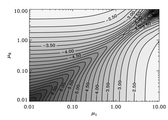
FIG. 2.: Logarithmic (base 10) contour plot of $\hat{Y}_{3/2}\equiv Y_{3/2}(g_{\ast s}/200)(T_{\rm R}/H_{\rm I})^{3}(a_{\rm R}/a_{\rm I})^{3}$, for $\Delta\eta/|\eta_{\rm I}|=1$, and for a transition into matter domination, in the plane $\mu_{1}-\mu_{2}$.

FIG. 3.: Dependence of $\hat{Y}_{3/2}\equiv Y_{3/2}(g_{\ast s}/200)(T_{\rm R}/H_{\rm I})^{3}(a_{\rm R}/a_{\rm I})^{3}$ on the effective mass of the gravitino in different cases: solid line $m/H\equiv\mu_{1}=\mu_{2}$, dotted line $m/H\equiv\mu_{2}$ and $\mu_{1}=0$, dashed line $m/H\equiv\mu_{1}$ and $\mu_{2}=0$, and in dash-dotted line, as a function of a constant mass term, equal in both inflation and matter domination eras. In each case, the transition is operated on a timescale $\Delta\eta/|\eta_{\rm I}|=1$ into matter domination.

The quantity of direct interest to us is $Y_{3/2}$, defined as the ratio of the number density of helicity$-3/2$ gravitinos to the entropy density at the time of reheating $\eta_{\rm R}$:

$$Y_{3/2}(\eta_{\rm R})=\frac{45}{4\pi^{4}g_{\ast s}}\left(\frac{a_{\rm I}H_{\rm I}}{a_{\rm R}T_{\rm R}}\right)^{3}\sum_{s=\pm}\int{\rm d}{\tilde{k}}{\tilde{k}}^{2}|\beta_{ks}|^{2},$$ (25)

where $g_{\ast s}$ is the effective number of degrees of freedom, $g_{\ast s}\simeq 229$ for the minimal supersymmetric standard model, $T_{\rm R}$ is the reheating temperature, $a_{\rm R}\equiv a(\eta_{\rm R})$, $a_{\rm I}\equiv a(\eta_{\rm I})$, and ${\tilde{k}}\equiv k/H_{\rm I}=k|\eta_{\rm I}|$.

Since $|\beta_{ks}|^{2}\leq 1$ is imposed by Pauli blocking, the integral in Eq. (25) is dominated by the high wavenumber modes. As a matter of fact, this integral diverges linearly, since $|\beta_{ks}|^{2}\propto k^{-2}$ for $k|\eta_{\rm I}|\gg 1$, according to Eq. (24). This divergence is unphysical, and results from the sudden transition approximation, as is well-known, for instance, in the case of gravitational waves production during inflation [19, 20]. The adiabatic theorem [17, 4] indeed implies that $|\beta_{ks}|^{2}$ falls off exponentially with $k$ beyond some cut-off $k_{\rm c}$ (see also Ref. [21] for a recent study). In effect, a numerical integration of the field equation shows that if the transition between inflation and radiation/matter domination is sufficiently smooth, an exponential cut-off appears, as shown in Fig. (1). Since the integral in Eq. (25) is proportional to $k_{\rm c}$ (provided $k_{\rm c}|\eta_{\rm I}|>1$), we will use numerical integration of the field equation for quantitative estimates, and the analytical solution to understand the behavior in various regimes of $k$, $\mu_{1}$, and $\mu_{2}$.

In Fig. (1), we compare the analytical (dashed line) and numerical solutions to $|\beta_{ks}|^{2}$ in the case where $\mu_{1}=0$ and $\mu_{2}=1$, and for a transition into matter domination. The exact value of the cut-off wavenumber $k_{c}$ depends on the duration $\Delta\eta$ of the transition between inflation and matter domination [17, 20], as indeed, the “degree of non-adiabaticity” of the transition is inversely proportional to $\Delta\eta$. Figure (1) shows that the analytical solution is an excellent approximation to the numerical solution for $k\lesssim k_{\rm c}$, even for $k_{\rm c}|\eta_{\rm I}|>1$. Furthermore, as expected, $k_{\rm c}\propto 1/\Delta\eta$, and therefore the number density in Eq. (25) also scales approximately as $1/\Delta\eta$. Indeed, as shown in Fig. (1), the analytical solution for the sudden transition corresponds to the numerical solution with the cut-off $k_{\rm c}$ cast to infinity.

In Fig. (2), we show a (base 10) logarithmic contour plot of $Y_{3/2}(g_{\ast s}/200)(T_{\rm R}/H_{\rm I})^{3}(a_{\rm R}/a_{\rm I})^{3}$ in the plane $\mu_{1},\mu_{2}$, assuming a transition with $\Delta\eta/|\eta_{\rm I}|=1$ into matter domination. A transition into radiation domination gives similar results. As $\mu_{1}=\mu_{2}\to+\infty$, the production is exponentially suppressed [see also Fig. (3)], in agreement with the adiabatic theorem. This can be seen in Eq. (24), at least in the limit where $k|\eta_{\rm I}|\ll 1$, for which $|\beta_{ks}|^{2}\propto\exp(-2\pi\mu_{1})$. In the limit $\mu_{1}\to 0$, with $\mu_{2}$ fixed, one has $Y_{3/2}\propto\mu_{1}^{2}$, and similarly for $\mu_{2}\to 0$, with $\mu_{1}$ fixed. Notably, $Y_{3/2}\to 0$ as $\mu_{1}\to 0$ and $\mu_{2}\to 0$, since a massless gravitino is conformally invariant. Finally, for a fixed $\mu_{1}$, the number density is not exponentially suppressed as $\mu_{2}\to+\infty$; indeed, Eq. (24) gives $|\beta_{ks}|^{2}\to 1/2$ when $\mu_{1}\to 0$ and $\mu_{2}\to+\infty$, for $k|\eta_{\rm I}|<1$. Since $k_{\rm c}$ is roughly proportional to max$(\mu_{1},\mu_{2})$, the number density increases linearly with $\mu_{2}$ in this limit. Note that this does not contradict the adiabatic theorem: as $\mu_{1}\to 0$ and $\mu_{2}\to+\infty$, for a fixed $\Delta\eta$, the transition becomes increasingly non-adiabatic, and particle production is not suppressed.

Finally, in Fig. (3), we show cuts of the previous contour plot, for $\mu_{1}=\mu_{2}$ [diagonal of Fig. (2)], for $\mu_{1}=0$ [$y-$axis of Fig. (2)], and for $\mu_{2}=0$ [$x-$axis of Fig. (2)], in each case for a transition into matter domination with $\Delta\eta/|\eta_{\rm I}|=1$. For the sake of completeness, we also include the result of a numerical integration for the case where the mass of the gravitino is constant and has the same value in both inflationary and matter dominated epochs, in dash-dotted line. Just like the case $\mu_{1}=\mu_{2}$, it shows exponential suppression as $m\gg H_{\rm I}$.

The number density of gravitationally produced gravitinos present at the time of reheating thus depends on several parameters, notably the effective mass terms during and after inflation, the duration of the transition from inflation to reheating, and the number of e-folds of reheating. The yield of gravitinos scales as the inverse of the transition timescale, which defines the degree of ”non-adiabaticity”, and decreases as $\exp(-3N_{\rm R})$, where $N_{\rm R}\equiv\ln(a_{\rm R}/a_{\rm I})$ is the number of e-folds of reheating, during which the gravitinos are diluted. These dependences make a direct comparison with the number density of gravitinos produced in particle interactions in reheating slightly delicate.

Let us first isolate the dependence on the mass terms and transition timescale in the fiducial quantity $\hat{Y}_{3/2}$, which is defined through: $Y_{3/2}=\hat{Y}_{3/2}(g_{\ast s}/200)^{-1}(H_{\rm I}/T_{\rm R})^{3}\exp(-3N_{\rm R})$; the quantity plotted in Figs (2) and (3) is $\hat{Y}_{3/2}$ (for $\Delta\eta=H_{\rm I}^{-1}$). The number of e-folds of reheating, and therefore $Y_{3/2}$, depend on the detailed mechanism of reheating, which is unfortunately not well known at present. In the most standard model of reheating [22], in which the inflaton slowly decays through its coherent oscillations, and the Universe is matter dominated, one obtains: $3N_{\rm R}\simeq 58.5+\ln\left[(H_{\rm I}/10^{13}\,{\rm GeV})^{2}(T_{\rm R}/10^{9}\,{\rm GeV})^{-4}(g_{\ast}/200)^{-1}\right]$. The dilution is therefore quite strong, and $Y_{3/2}\simeq 3\times 10^{-14}\hat{Y}_{3/2}(H_{\rm I}/10^{13}\,{\rm GeV})(T_{\rm R}/10^{9}\,{\rm GeV})$. More generally, if reheating takes place in an era dominated by an equation of state of the form $p=w\rho$, the above number of e-folds is reduced by a factor $1/(1+w)$; for $w=1/3$, for instance, which corresponds to a relativistic fluid, one finds: $Y_{3/2}\simeq 9\times 10^{-8}\hat{Y}_{3/2}(H_{\rm I}/10^{13}\,{\rm GeV})^{3/2}(g_{\ast s}/200)^{-1/4}$, and the number density produced becomes independent of the reheating temperature. It was pointed out in Ref. [19] that in a general case, oscillations of an inflaton in a potential $\sim\lambda\phi^{2n}$ would yield an equation state with $w\simeq(n-1)/(n+1)$ after averaging out over an oscillation period. Thus, in particular, for chaotic inflation with a potential $\lambda\phi^{4}$, the Universe is indeed dominated by a relativistic fluid during reheating ($w=1/3$).

The ratio $Y^{\rm R}_{3/2}$ of the number density of gravitinos produced in particle interactions during reheating to the entropy density is, up to logarithmic corrections [11]: $Y^{\rm R}_{3/2}\approx 3.7\times 10^{-13}(T_{\rm R}/10^{9}\,{\rm GeV})(g_{\ast s}/200)^{-3/2}$. Therefore, the ratio $Y_{3/2}/Y^{\rm R}_{3/2}$ of these two yields, assuming that reheating takes place in a matter dominated era is:

$$\frac{Y_{3/2}}{Y^{\rm R}_{3/2}}\simeq 0.1\,\hat{Y}_{3/2}\,\left(\frac{H_{\rm I}}{10^{13}\,{\rm GeV}}\right)\left(\frac{g_{\ast s}}{200}\right)^{3/2},$$ (26)

and according to Fig. (3), $\hat{Y}_{3/2}\approx 10^{-3}\mu^{2}_{1,2}(\Delta\eta/|\eta_{\rm I}|)^{-1}$, if $\mu_{1}=0$ and $\mu_{2}=1$ or the reverse. This constitutes our main result. If throughout reheating, the Universe is dominated by a relativistic equation of state, it becomes:

$$\frac{Y_{3/2}}{Y^{\rm R}_{3/2}}\simeq 2\times 10^{5}\hat{Y}_{3/2}\left(\frac{H_{\rm I}}{10^{13}\,{\rm GeV}}\right)^{3/2}\left(\frac{T_{\rm R}}{10^{9}\,{\rm GeV}}\right)^{-1}\left(\frac{g_{\ast s}}{200}\right)^{5/4}.$$ (27)

Whereas the ratio of the two production yields is independent of the reheating temperature when the Universe is matter dominated during reheating, it becomes inversely proportional to $T_{\rm R}$ when $w=1/3$ (relativistic fluid). Therefore, if gravitational production is efficient, i.e., if $m\sim H$ during or after inflation, a low reheating temperature does not exclude a strong gravitino problem.

Let us now discuss the magnitude of $\hat{Y}_{3/2}$. As seen in Fig. (3), one probably has $\hat{Y}_{3/2}\lesssim 10^{-3}$ if $\Delta\eta=H_{\rm I}^{-1}$, where the upper limit corresponds to $\mu_{1}=0$ and $\mu_{2}=1$, or $\mu_{1}=1$ and $\mu_{2}=0$. Therefore, for reheating in a matter dominated era, one finds that the production of gravitinos out of the vacuum is less efficient than that during reheating, provided $\Delta\eta\gtrsim 10^{-4}H_{\rm I}^{-1}$. In the other limit, where the Universe is dominated by a relativistic equation of state during reheating, one finds that gravitational production can be much more efficient that reheating production of gravitinos, by a factor $\sim 10^{2}\mu^{2}_{1,2}(\Delta\eta/|\eta_{\rm I}|)^{-1}(T_{\rm R}/10^{9}\,{\rm GeV})^{-1}$.

Finally, an order of magnitude estimate for $\Delta\eta$ is $\phi/\phi^{\prime}$ ($\phi$ is the inflaton field) taken at the point at which the slow-roll approximation breaks down, i.e. where $\dot{\phi}^{2}/2\sim V(\phi)$ (a dot denotes differentiation with respect to cosmic time). This gives $\Delta\eta\approx 2(\phi/M_{\rm Pl})|\eta_{\rm I}|$, with $M_{\rm Pl}\equiv(8\pi)^{1/2}m_{\rm Pl}$ the Planck mass. Therefore, $\Delta\eta\sim|\eta_{\rm I}|$ for scenarios of the chaotic type, and $\Delta\eta\ll|\eta_{\rm I}|$ for scenarios of the new inflation type with small field values; quite possibly, in this latter case, $\Delta\eta<10^{-4}|\eta_{\rm I}|$ [20].

In new inflation, therefore, the gravitational production cannot be neglected if $\mu_{1}\sim 0$ and $\mu_{2}\sim 1$ (or the reverse), $\phi\lesssim 10^{-4}M_{\rm Pl}$ at the end of slow-roll, and $H_{\rm I}\sim 10^{13}\,$GeV. Moreover, if reheating proceeds faster than in the “standard” model (matter domination), such as in $\lambda\phi^{4}$ chaotic inflation, gravitational production of gravitinos can become more efficient than reheating production. If gravitational production dominates, cosmological bounds on the gravitino abundance at the time of Big Bang nucleosynthesis should be turned into upper limits on the effective mass terms of the gravitino during and after inflation, as gravitational production is suppressed as $(m/H_{\rm I})^{2}$ if $m<H_{\rm I}$.

IV Discussion

We discussed the conformal behavior of the gravitino in a spatially flat FRW background spacetime. We obtained the linearized field equation for the helicity $\pm 3/2$ components, which reduces to a Dirac like equation in curved spacetime. A massive gravitino is not conformally invariant, and cosmological particle production ensues, through the amplification of the vacuum fluctuations by the non-static background metric. We assumed that the gravitino effective mass is proportional to the Hubble constant, and used the technique of Bogoliubov transforms to calculate the ratio $Y_{3/2}$ of the number density of gravitinos to the entropy density at the time of reheating. This quantity depends on the effective mass of the gravitino during and after inflation, on the Hubble constant at the exit of inflation ($H_{\rm I}$), on the duration of the transition between inflation and radiation/matter domination ($\Delta\eta$), and on the number of e-folds of reheating. Notably, $Y_{3/2}$ scales as the inverse of the transition timescale, which defines the degree of “non-adiabaticity” of the transition during which gravitinos are produced. The comparison of the gravitational production of gravitinos to production in reheating depends on the details of the mechanism of reheating, during which the gravitationally produced gravitinos are strongly diluted.

If we assume that the gravitino mass is of order of the Hubble constant during or after inflation, that $H_{\rm I}\sim 10^{13}\,$GeV, and that the Universe is matter dominated throughout reheating, gravitational production is generically less efficient than production in reheating interactions, provided the transition is not too abrupt, i.e. $\Delta\eta\gtrsim 10^{-4}H_{\rm I}^{-1}$. However, in scenarios of new inflation, one can find $\Delta\eta\lesssim 10^{-4}H_{\rm I}^{-1}$, in which case gravitational production would turn out to produce as many gravitinos, or more, than reheating interactions. Similarly, if reheating proceeds faster, for instance if the Universe is dominated by a relativistic fluid during reheating, as happens in e.g., chaotic inflation with a potential $\lambda\phi^{4}$, the number density of gravitinos produced out of the vacuum exceeds, possibly by a large factor, the density of gravitinos produced in particle interactions during reheating. It must be stressed that in the above, we assumed the effective mass $m$ of the gravitino to be of order the Hubble constant, either during or after inflation. If not, gravitational production is suppressed as $(m/H_{\rm I})^{2}$.

To conclude, let us briefly address the particular case of pre-Big-Bang string cosmology [6], in which particle production out of the vacuum has been studied extensively [23, 24], but not for spin$-3/2$. In this scenario, one expects that, to leading order, the gravitino mass term vanishes during inflation, if the only dynamical field is the axion-dilaton field, as indeed, the tree level superpotential of string-inspired supergravity does not receive contributions from the dilaton. Similarly, $m=0$ also in the post-inflationary phase (if only the axion-dilaton field is considered), at least until a non perturbative superpotential for the dilaton sets in, or until supersymmetry breaking takes place. If we assume that the gravitino is also massless during the so-called stringy phase, it then couples to the axion-dilaton field only through the Kähler connection. The field equation Eq. (10) then decouples into two first order differential equations for the mode functions $h_{ss}$ and $g_{ss}$, whose solutions are written as in flat-space up to a time-dependent phase which depends on the Kähler connection. If the initial state corresponds to the conformal vacuum as $\eta\to-\infty$, then $h^{\rm in}_{++}=g^{\rm in}_{--}=0$. Since we assume that the gravitino remains massless after inflation, conformal triviality also holds as $\eta\to+\infty$, and $h^{\rm out}_{++}=g^{\rm out}_{--}=0$. From Eq. (16), it is then obvious that $\beta_{ks}=0$, i.e. no particle production takes place.

At the next level of approximation, one should consider moduli fields, take into account higher order corrections to the effective action in the stringy phase, and/or introduce a non-perturbative superpotential to stabilize the dilaton in the FRW phase. This would lead, quite presumably, to the appearance of an effective mass for the gravitino. Unfortunately, these effects are difficult to implement, because the underlying dynamics or the physics remain poorly known. To give an example of what could be obtained, let us assume that the gravitino is massless during the pre-Big Bang and stringy phases, and that it acquires a mass after the exit in the FRW era. Then the methods and results of the previous section can easily be transposed to this scenario, since the gravitino, being massless in the pre-FRW eras, is insensitive to the background dynamics. It is easy to verify that if the exit in the FRW phase takes place at a scale $H_{\rm I}\sim 10^{17}\,$GeV, as has been advocated recently [24], gravitational and reheating production of gravitinos become of the same order, even if the Universe is matter dominated throughout reheating, provided $m\sim H_{\rm I}$.

However, reheating in pre-Big Bang cosmology is not expected to proceed through coherent oscillations of the “inflaton”, and the above estimate could turn out to be naive. A detailed study of the mechanism of reheating in pre-Big Bang cosmology thus appears mandatory. Depending on how fast reheating proceeds, and what temperature is achieved, this could lead to a strong gravitino problem (which one would naively expect if $H_{\rm I}\sim 10^{17}\,$GeV), which would thus require: $m_{3/2}\gtrsim 10^{4}\,$GeV for an unstable gravitino, or $m_{3/2}\lesssim 2\,$keV for a stable gravitino. A more detailed study of this problem is left for further work.

Note added

Upon completion of this paper, we became aware of a related work by A. L. Maroto and A. Mazumdar (“Production of spin 3/2 particles from vacuum fluctuations”, hep-ph/9904206). These authors obtained the field equation for helicity 3/2 gravitinos, assuming $\gamma^{\mu}\Psi_{\mu}=0$ (which projects out helicity 1/2 modes), and calculated the amplification of vacuum fluctuations, using the technique of Bogoliubov transforms. They applied their technique to the production of gravitinos in preheating. In this respect, their work and ours are complementary: gravitational production during inflation generically produces particles with wavenumber $k\lesssim H_{\rm I}$, while in preheating, the production takes place for modes with $k\gtrsim H_{\rm I}$.

After the present paper was submitted, two other related studies appeared: R. Kallosh, L. Kofman, A. Linde and A. Van Proeyen (“Gravitino production after inflation”, hep-ph/9907124) studied the problem of gravitino production during inflation and during preheating, for both helicity 1/2 and helicity 3/2 modes. Their important work shows that the helicity 1/2 modes are not conformally invariant even if they are massless, and that their production in preheating can be very large. The paper by G. F. Giudice, A. Riotto and I. Tkachev (“Non-thermal production of dangerous relics in the early Universe”, hep-ph/9907510) reaches similar conclusions.

Notations

We write $\gamma_{\mu}$ a general relativistic Dirac matrix, and $\gamma_{a}=e_{a}^{\mu}\gamma_{\mu}$, or, if confusion could arise, $\hat{\gamma}_{a}$, a (constant) flat-space Dirac matrix. We define: $\sigma_{ab}=\frac{1}{2}[\gamma_{a},\gamma_{b}]$. The Dirac matrices are written in the Weyl representation:

$$\gamma^{a}=-i\left(\begin{array}[]{cc}0&\bar{\sigma}_{a}\\ \bar{\sigma}_{a}&0\\ \end{array}\right),$$ (28)

with: $\sigma_{a}=(1,\mathchoice{{\hbox{\boldmath$\displaystyle\sigma$}}}{{\hbox{\boldmath$\textstyle\sigma$}}}{{\hbox{\boldmath$\scriptstyle\sigma$}}}{{\hbox{\boldmath$\scriptscriptstyle\sigma$}}})$, and $\bar{\sigma}_{a}=(1,-\mathchoice{{\hbox{\boldmath$\displaystyle\sigma$}}}{{\hbox{\boldmath$\textstyle\sigma$}}}{{\hbox{\boldmath$\scriptstyle\sigma$}}}{{\hbox{\boldmath$\scriptscriptstyle\sigma$}}})$, and the $\textstyle\sigma$ are flat-space Pauli matrices. We also define: $\gamma_{5}=i\hat{\gamma}_{0}\hat{\gamma}_{1}\hat{\gamma}_{2}\hat{\gamma}_{3}$.

Our choice of vierbein for the FRW background is: $e_{\mu}^{{}a}=a(\eta)$, $e^{\mu}_{{}a}=a(\eta)^{-1}$. The spin connection, without $\Psi$ torsion, is then:

$$\frac{1}{4}\omega_{0}^{ab}\sigma_{ab}=0,\,\,\,\,\frac{1}{4}\omega_{i}^{ab}\sigma_{ab}=\frac{1}{2}{\cal H}\gamma_{i}\gamma^{0},$$ (29)

where we defined ${\cal H}=a^{\prime}/a$. We define the helicity operator $\mathchoice{{\hbox{\boldmath$\displaystyle\epsilon$}}}{{\hbox{\boldmath$\textstyle\epsilon$}}}{{\hbox{\boldmath$\scriptstyle\epsilon$}}}{{\hbox{\boldmath$\scriptscriptstyle\epsilon$}}}^{\rm L}\mathchoice{{\hbox{\boldmath$\displaystyle\sigma$}}}{{\hbox{\boldmath$\textstyle\sigma$}}}{{\hbox{\boldmath$\scriptstyle\sigma$}}}{{\hbox{\boldmath$\scriptscriptstyle\sigma$}}}$ for a Weyl spinor of momentum $\textstyle k$, where $\mathchoice{{\hbox{\boldmath$\displaystyle\epsilon$}}}{{\hbox{\boldmath$\textstyle\epsilon$}}}{{\hbox{\boldmath$\scriptstyle\epsilon$}}}{{\hbox{\boldmath$\scriptscriptstyle\epsilon$}}}^{\rm L}$ is the unitary vector along $\textstyle k$. We then define $\chi_{+}(\mathchoice{{\hbox{\boldmath$\displaystyle k$}}}{{\hbox{\boldmath$\textstyle k$}}}{{\hbox{\boldmath$\scriptstyle k$}}}{{\hbox{\boldmath$\scriptscriptstyle k$}}})$ and $\chi_{-}(\mathchoice{{\hbox{\boldmath$\displaystyle k$}}}{{\hbox{\boldmath$\textstyle k$}}}{{\hbox{\boldmath$\scriptstyle k$}}}{{\hbox{\boldmath$\scriptscriptstyle k$}}})$ as the eigenspinors of $\mathchoice{{\hbox{\boldmath$\displaystyle\epsilon$}}}{{\hbox{\boldmath$\textstyle\epsilon$}}}{{\hbox{\boldmath$\scriptstyle\epsilon$}}}{{\hbox{\boldmath$\scriptscriptstyle\epsilon$}}}^{\rm L}\mathchoice{{\hbox{\boldmath$\displaystyle\sigma$}}}{{\hbox{\boldmath$\textstyle\sigma$}}}{{\hbox{\boldmath$\scriptstyle\sigma$}}}{{\hbox{\boldmath$\scriptscriptstyle\sigma$}}}$ with respective helicity $+1/2$ and $-1/2$: $\mathchoice{{\hbox{\boldmath$\displaystyle\epsilon$}}}{{\hbox{\boldmath$\textstyle\epsilon$}}}{{\hbox{\boldmath$\scriptstyle\epsilon$}}}{{\hbox{\boldmath$\scriptscriptstyle\epsilon$}}}^{\rm L}\mathchoice{{\hbox{\boldmath$\displaystyle\sigma$}}}{{\hbox{\boldmath$\textstyle\sigma$}}}{{\hbox{\boldmath$\scriptstyle\sigma$}}}{{\hbox{\boldmath$\scriptscriptstyle\sigma$}}}\,\chi_{\pm}(\mathchoice{{\hbox{\boldmath$\displaystyle k$}}}{{\hbox{\boldmath$\textstyle k$}}}{{\hbox{\boldmath$\scriptstyle k$}}}{{\hbox{\boldmath$\scriptscriptstyle k$}}})=\pm\chi_{\pm}(\mathchoice{{\hbox{\boldmath$\displaystyle k$}}}{{\hbox{\boldmath$\textstyle k$}}}{{\hbox{\boldmath$\scriptstyle k$}}}{{\hbox{\boldmath$\scriptscriptstyle k$}}})$. We decompose a four component spinor $\psi(\eta,\mathchoice{{\hbox{\boldmath$\displaystyle k$}}}{{\hbox{\boldmath$\textstyle k$}}}{{\hbox{\boldmath$\scriptstyle k$}}}{{\hbox{\boldmath$\scriptscriptstyle k$}}})$ in eigenstates of helicity [11], $\psi(\eta,\mathchoice{{\hbox{\boldmath$\displaystyle k$}}}{{\hbox{\boldmath$\textstyle k$}}}{{\hbox{\boldmath$\scriptstyle k$}}}{{\hbox{\boldmath$\scriptscriptstyle k$}}})=\psi_{+}(\eta,\mathchoice{{\hbox{\boldmath$\displaystyle k$}}}{{\hbox{\boldmath$\textstyle k$}}}{{\hbox{\boldmath$\scriptstyle k$}}}{{\hbox{\boldmath$\scriptscriptstyle k$}}})+\psi_{-}(\eta,\mathchoice{{\hbox{\boldmath$\displaystyle k$}}}{{\hbox{\boldmath$\textstyle k$}}}{{\hbox{\boldmath$\scriptstyle k$}}}{{\hbox{\boldmath$\scriptscriptstyle k$}}})$, with:

$$\psi_{s}(\eta,\mathchoice{{\hbox{\boldmath$\displaystyle k$}}}{{\hbox{\boldmath$\textstyle k$}}}{{\hbox{\boldmath$\scriptstyle k$}}}{{\hbox{\boldmath$\scriptscriptstyle k$}}})=\left(\begin{array}[]{c}h_{s}(\eta)\chi_{s}(\mathchoice{{\hbox{\boldmath$\displaystyle k$}}}{{\hbox{\boldmath$\textstyle k$}}}{{\hbox{\boldmath$\scriptstyle k$}}}{{\hbox{\boldmath$\scriptscriptstyle k$}}})\\ sg_{s}(\eta)\chi_{s}(\mathchoice{{\hbox{\boldmath$\displaystyle k$}}}{{\hbox{\boldmath$\textstyle k$}}}{{\hbox{\boldmath$\scriptstyle k$}}}{{\hbox{\boldmath$\scriptscriptstyle k$}}})\\ \end{array}\right),\,\,\,s=\pm,$$ (30)

where $h_{s}(\eta)$, and $g_{s}(\eta)$ are (scalar) functions of conformal time. The eigenspinors $\chi_{+}$ and $\chi_{-}$ verify, in particular: $\chi_{s}^{\dagger}\chi_{s^{\prime}}=\delta_{ss^{\prime}}$. In Section II, we perform a similar decomposition for the spinor-vector in terms of the mode functions $h_{ms}(\eta)$, where $m=L,+,-$ denotes the helicity of the polarization vector, and $s=\pm$ denotes the spinor helicity.

Finally, we define the charge conjugation operator: $C=i\hat{\gamma}^{2}\hat{\gamma}^{0}$, and the conjugate $\psi^{\rm C}$ of a spinor $\psi$: $\psi^{\rm C}=iC\hat{\gamma}^{0}\Psi^{\ast}$. One can show that: $i\sigma_{2}\chi_{s}^{\ast}=-s\chi_{s}$, where $s=\pm$. It is then easy to show that the conjugate of a spinor $\psi_{s}(\eta,-\mathchoice{{\hbox{\boldmath$\displaystyle k$}}}{{\hbox{\boldmath$\textstyle k$}}}{{\hbox{\boldmath$\scriptstyle k$}}}{{\hbox{\boldmath$\scriptscriptstyle k$}}})$, with helicity $s$, and momentum $-\mathchoice{{\hbox{\boldmath$\displaystyle k$}}}{{\hbox{\boldmath$\textstyle k$}}}{{\hbox{\boldmath$\scriptstyle k$}}}{{\hbox{\boldmath$\scriptscriptstyle k$}}}$, is:

$$\Psi^{\rm C}_{s}(\eta,-\mathchoice{{\hbox{\boldmath$\displaystyle k$}}}{{\hbox{\boldmath$\textstyle k$}}}{{\hbox{\boldmath$\scriptstyle k$}}}{{\hbox{\boldmath$\scriptscriptstyle k$}}})=i\left(\begin{array}[]{c}g_{s}^{\ast}\chi_{s}\\ -sh_{s}^{\ast}\chi_{s}\\ \end{array}\right).$$ (31)

This identity is useful in deriving the normalization identities of the gravitino operator in Section II.

REFERENCES

[1] H. Pagels and J. Primack, Phys. Rev. Lett. 48 (1982) 223;
S. Weinberg, Phys. Rev. Lett. 48 (1982) 1303.
[2] J. Ellis, A. D. Linde and D. V. Nanopoulos,
Phys. Lett. 118B (1982) 59.
[3] D. Nanopoulos, K. A. Olive and M. Srednicki,
Phys. Lett. 127B (1983) 30; L. Krauss, Nuc. Phys. B227 (1983) 556;
M. Yu. Khlopov and A. D. Linde, Phys. Lett. 118B (1984) 265; J. Ellis,
J. E. Kim and D. V. Nanopoulos, Phys. Lett. 145B (1984) 181; J. Ellis,
J. Hagelin, D. Nanopoulos, K. A. Olive and M. Srednicki,
Nuc. Phys. B238 (1984) 453; R. Juszkiewicz, J. Silk and A. Stebbins,
Phys. Lett. 158B (1985) 463; S. Dimopoulos, R. Esmailzadeh, L. J. Hall
and G. D. Starkman, Nucl. Phys. B311 (1989) 699; T. Moroi, H. Murayama
and M. Yamaguchi, Phys. Lett. 303B (1993) 289; T. Moroi and
T.Yanagida, Prog. Theor. Phys. 93 (1995) 879.
[4] N. D. Birrell and P. C. W. Davies, Quantum fields in
curved space (Cambridge University Press, 1982).
[5] K. A. Olive, Phys. Rep. 190 (1990) 307; D. H. Lyth and
A. Riotto, Phys. Rep., in press (1999), e-print hep-ph/9807278.
[6] M. Gasperini and G. Veneziano, Astropart. Phys. 1 (1993) 317;
collection of papers at http://www.to.infn.it/gasperin/.
[7] D. H. Lyth, D. Roberts and M. Smith, Phys. Rev. D57
(1998) 7120.
[8] L. P. Grishchuk and A. D. Popova, Zh. Eksp. Teor. Fiz 77
(1979) 1665 [Sov. Phys. JETP 50 (1979) 835].
[9] S. Deser and B. Zumino, Phys. Lett. 62B (1976) 335.
[10] S. Deser and B. Zumino, Phys. Rev. Lett. 38 (1977) 1433.
[11] T. Moroi, PhD thesis (1995) Tohoku University (Japan),
e-print hep-ph/9503210.
[12] L. Parker, Phys. Rev. D3 (1971) 346.
[13] Y. Kluger, J. M. Eisenberg, B. Svetitsky, F. Cooper and
E. Mottola, Phys. Rev. D45 (1992) 4659.
[14] M. Dine, L. Randall and S. Thomas, Phys. Rev. Lett. 75 (1995)
398.
[15] G. Felder, L. Kofman and A. Linde, e-print hep-ph/9903350.
[16] E. Stewart, Phys. Lett. 391B (1997) 34; Phys. Rev. D56
(1997) 2019.
[17] L. Parker, Phys. Rev. 183 (1969) 1057.
[18] I. S. Gradshteyn and I. M. Ryzhik, Table of integrals,
series and products (Academic Press, 1963); M. Abramowitz and L. A. Stegun,
Handbook of mathematical functions (National Bureau of Standards, 1964).
[19] L. H. Ford, Phys. Rev. D35 (1987) 2955.
[20] B. Allen, Phys. Rev. D37 (1987) 2078; V. Sahni,
Phys. Rev. D42 (1990) 453; L. P. Grishchuk, Phys. Rev. D48 (1993)
3513; M. R. de Garcia Maia, Phys. Rev. D48 (1993) 647;
R. G. Moorhouse, A. B. Henriques and L. E. Mendes, Phys. Rev. D50
(1994) 2600.
[21] D. J. H. Chung, E. W. Kolb and A. Riotto,
Phys. Rev. D59 (1999) 023501.
[22] E. W. Kolb and M. S. Turner, The Early Universe
(Addison-Wesley, 1991); A. Linde, Particle Physics and Inflationary
Cosmology (Contemporary Concepts in Physics, Harwood, 1990).
[23] R. Brustein and M. Hadad, Phys. Rev. D57 (1998) 712.
[24] A. Buonanno, K. A. Meissner, C. Ungarelli and
G. Veneziano, JHEP 9801 (1998) 004.