Abstract

$U_{A}(1)$ symmetry breaking is studied by introducing the flavor mixing interaction proposed by Kobayashi, Maskawa and ’t Hooft. Combining the one gluon exchange interaction, the rainbow like Schwinger–Dyson equation and the ladder like Bethe–Salpeter equation are derived. The anomalous PCAC relation in the framework of this approximation is considered. The masses of the pseudoscalar mesons $\pi,\eta$ and $\eta^{\prime}$ are calculated. It is found that the pion mass is not sensitive to the strength of the flavor mixing interaction. On the other hand, the masses of $\eta$ and $\eta^{\prime}$ are reproduced by a relatively weak flavor mixing interaction, for which the chiral symmetry breaking is dominantly induced by the soft-gluon exchange interaction. The decay constants are calculated and the anomalous PCAC relation is numerically checked. It is found that the flavor structures of the $\eta$ and $\eta^{\prime}$ mesons significantly depend on their masses and therefore it is quetionable to define a flavor mixing angle for $\eta$ and $\eta^{\prime}$.

1 Introduction

It is known that the classical QCD lagrangian is invariant under the $U_{L}(3)\times U_{R}(3)$ symmetry except for the quark mass term, and this symmetry is broken down to the $U_{V}(3)$ spontaneously in the low-energy QCD. In this case, the number of the Nambu-Goldstone bosons should be nine. However, the number of the observed light pseudoscalar mesons is eight. The ninth pseudoscalar meson, $\eta^{\prime}$ meson, is heavier than the other octet pseudoscalar mesons ($\pi^{0}$, $\pi^{+}$, $\pi^{-}$, $K^{+}$, $K^{-}$, $K^{0}$, $\overline{K}^{0}$ and $\eta$) which are well identified with the Nambu–Goldstone bosons. This is the well-known $U_{A}(1)$ problem [1]. It is solved by realizing that the $U_{A}(1)$ symmetry is broken by the anomaly. The phenomena related to the $U_{A}(1)$ anomaly in the low-energy QCD have been studied in the following approaches.

The first one is the $1/N_{C}$ expansion approach [2, 3]. The key point is that the effect of the $U_{A}(1)$ anomaly is higher order in the $1/N_{C}$ expansion and the low-energy effective lagrangian of QCD has been derived [4]. Recently, the expansion in powers of $1/N_{C}$, momenta and quark masses was extended to the first non-leading order [5] and the reasonable description of the nonet pseudoscalar mesons was obtained.

The second is the instanton approach [6]. The instanton is a classical solution of the Euclidean Yang–Mills equation and may contribute a large weight in the Feynman path integration. In the presence of the light quarks, instantons are associated with fermionic zero modes which give rise to the $U_{A}(1)$ symmetry breaking. In the dilute instanton gas approximation, the $U_{A}(1)$ breaking 6-quark flavor determinant interaction was derived in the three flavor case [7]. This approach has been developed to the instanton liquid picture of the QCD vacuum [8]. In this picture, the instanton plays a crucial role in understanding not only the $U_{A}(1)$ anomaly but also the spontaneous breaking of the chiral symmetry itself.

In the third approach, the effective low-energy quark models of QCD were used to study the structure of the hadrons. The introduction of the instanton induced six-quark interaction to the effective quark model is one of the handy way to incorporate the the $U_{A}(1)$ breaking effects in the low-energy effective quark model of QCD. The Nambu-Jona-Lasinio (NJL) model [9] is one of the simplest and widely used model in studying the structure of the Nambu-Goldstone bosons. Using the three-flavor NJL model with the instanton induced six quark interaction, properties of the nonet pseudoscalar mesons were investigated [10]. A shortcoming of this approach is that the $\eta^{\prime}$ mass has unphysical imaginary part associated with the unphysical decay channel $\eta^{\prime}\rightarrow\bar{q}q$. Recent study of the radiative decays of the $\eta$ meson in the NJL model has shown that the observed values of the mass and radiative decay amplitudes are reproduced well with a rather strong $U_{A}(1)$ breaking interaction [11]. Such strong $U_{A}(1)$ breaking may be consistent with the instanton liquid picture of the QCD vacuum.

In contrast with the instanton liquid model, the study of the QCD Schwinger-Dyson (SD) equation for the quark propagator in the improved ladder approximation (ILA) has shown that the spontaneous breaking of the chiral symmetry is explained by simply extrapolating the running coupling constant from the perturbative high-energy region to the low-energy region [12].

Then, the Bethe-Salpeter (BS) equation for the $J^{PC}=0^{-+}$ $q\bar{q}$ channel has been solved in the ILA and the existence of the Nambu-Goldstone pion has been confirmed [13]. The numerical predictions of the pion decay constant $f_{\pi}$ and the quark condensate $\langle\overline{\psi}\psi\rangle$ are rather good. It has been also shown that the BS amplitude shows the correct asymptotic behavior as predicted by the operator product expansion (OPE) in QCD [14]. The masses and decay constants for the lowest lying scalar, vector and axial-vector mesons have been evaluated by calculating the two point correlation functions for the composite operators $\overline{\psi}M\psi$. The obtained values are in good agreement with the observed ones [15].

Recently, the current quark mass term has been introduced in the studies of the BS amplitudes in the ILA [16] and the reasonable values of the pion mass, the pion decay constant and the quark condensate have been obtained with a rather large $\Lambda_{\rm QCD}$. It has been also shown that the pion mass square and the pion decay constant are almost proportional to the current quark mass up to the strange quark mass region.

Since the $\eta$ and $\eta^{\prime}$ system is expected to be sensitive to the $U_{A}(1)$ anomaly, the study of the $\eta$ and $\eta^{\prime}$ structure may give us information on the roles of the $U_{A}(1)$ anomaly in the low-energy QCD. The purpose of this paper is to study the properties of the $\eta$ and $\eta^{\prime}$ mesons by solving the coupled channel BS equation in the ILA. The effect of the $U_{A}(1)$ anomaly is introduced by the instanton induced six-quark determinant interaction. The instanton size effects are taken into account by the form factor of the interaction vertices. It guarantees the right asymptotic behavior of the solutions of the SD and BS equations.

There have been many studies of the pion BS amplitude using the effective models of QCD and /or the approximation schemes of QCD [17]. As for the $\eta$ and $\eta^{\prime}$ system, Jain and Munczek model [18] has been applied to them [19]. They have introduced the effect of the $U_{A}(1)$ anomaly by simply adding the additional mass term in the flavor singlet pseudoscalar meson channel by hand and the reasonable values of the masses and decay constants have been obtained.

It is known that the introduction of the two gluon exchange diagrams in the calculation of the $\eta$ and $\eta^{\prime}$ BS amplitudes beyond the ladder approximation do not break the $U_{A}(1)$ symmetry with the perturbative gluon propagator. Recently, it has been shown that if the gluon propagator has the strong infrared singularity, the $U_{A}(1)$ symmetry breaks [20]. The relaton between this approach and the instanton approach is not clear.

The paper is organized as follows. In Sec. 2 we explain the model Lagrangian we have used in the present study. In Sec. 3 the Conwall-Jackiw-Tomboulis (CJT) effective action [21] calculated from our model Lagrangian is presented. The SD and BS equations are derived from the CJT effective action in Sec. 4 and Sec. 5. In Sec. 6 the meson decay constant is derived. In Sec. 7 the Nambu-Goldstone solution of the BS equation is derived and the anomalous PCAC relation is discussed in Sec. 8. Sec. 9 is devoted to the numerical results. Finally, summary and concluding remarks are given in Sec.10.

2 Model

We use the flavor three $(N_{F}=3)$ effective model whose lagrangian density is given by

$${\cal L}[\psi,\overline{\psi}]:=\overline{\psi}f(\partial^{2})(i{\rm\ooalign{\hfil$/$\hfil\crcr\hbox{$\partial$}}}-m_{0})\psi+{\cal L}_{\rm GE}[\psi,\overline{\psi}]+{\cal L}_{\rm FM}[\psi,\overline{\psi}],$$ (1)

$$\psi:=(u,d,s)^{T}$$ (2)

where $f(\xi)$ is a cut-off function defined by [16]

$$f(\xi)=1+M\theta(\xi-\Lambda_{\rm UV}^{2}),\quad M\to\infty.$$ (3)

$m_{0}$ denotes a diagonal quark mass matrix $m_{0}={\rm diag}(m_{q},m_{q},m_{s})$ under the assumption of the isospin invariance. ${\cal L}_{\rm GE}$ denotes a gluon exchange interaction

$${\cal L}_{\rm GE}[\psi,\overline{\psi}](x) := -\frac{1}{2}\int_{pp^{\prime}qq^{\prime}}{\cal K}^{mm^{\prime},nn^{\prime}}(p,p^{\prime};q,q^{\prime})$$ (4)

$${}\times\overline{\psi}_{m}(p)\psi_{m^{\prime}}(p^{\prime})\overline{\psi}_{n}(q)\psi_{n^{\prime}}(q^{\prime})e^{-i(p+p^{\prime}+q+q^{\prime})x}\,,$$

$${\cal K}^{mm^{\prime},nn^{\prime}}(p,p^{\prime};q,q^{\prime}) = \bar{g}^{2}\left((\frac{p_{E}-q_{E}^{\prime}}{2})^{2},(\frac{q_{E}-p_{E}^{\prime}}{2})^{2}\right)$$ (5)

$$\times iD^{\mu\nu}\left(\frac{p+p^{\prime}}{2}-\frac{q+q^{\prime}}{2}\right)(\gamma_{\mu}T^{a})^{mm^{\prime}}(\gamma_{\nu}T^{a})^{nn^{\prime}}$$

where $\int_{p}$ denotes $\int\frac{d^{4}p}{(2\pi)^{4}}$ and $p_{E}$ represents the Euclidean momentum. The indeces $m,n,\dots$ represent combined indeces in the color, flavor and Dirac spaces. In Eq.(5) we employ the Landau gauge gluon propagator,

$$iD^{\mu\nu}(k)=\left(g^{\mu\nu}-\frac{k^{\mu}k^{\nu}}{k^{2}}\right)\frac{-1}{k^{2}},$$ (6)

and the Higashijima–Miransky type running coupling constant $\bar{g}^{2}$ defined as follows.

$$\bar{g}^{2}(p_{E}^{2},q_{E}^{2})=\theta(p_{E}^{2}-q_{E}^{2})g^{2}(p_{E}^{2})+\theta(q_{E}^{2}-p_{E}^{2})g^{2}(q_{E}^{2}),$$ (7)

with

$$g^{2}(p_{E}^{2}):=\left\{\begin{array}[]{ll}\displaystyle{\frac{1}{\beta_{0}}\frac{1}{1+t}}&\mbox{ for }t_{\rm IF}\leq t\\ \mbox{}&\\ \displaystyle{\frac{1}{2\beta_{0}}\frac{1}{(1+t_{\rm IF})^{2}}\left[3t_{\rm IF}-t_{0}+2-\frac{(t-t_{0})^{2}}{t_{\rm IF}-t_{0}}\right]}&\mbox{ for }t_{0}\leq t\leq t_{\rm IF}\\ \mbox{}&\\ \displaystyle{\frac{1}{2\beta_{0}}\frac{3t_{\rm IF}-t_{0}+2}{(1+t_{\rm IF})^{2}}}&\mbox{ for }t\leq t_{0}\end{array}\right.,$$ (8)

$$t:=\ln\frac{p_{E}^{2}}{\Lambda_{\rm QCD}^{2}}-1,$$ (9)

$$\beta_{0}:=\frac{1}{(4\pi)^{2}}\frac{11N_{C}-2N_{f}}{3}.$$ (10)

In Eq.(8) the infrared cut-off $t_{\rm IF}$ is introduced. Above $t_{\rm IF}$, $g^{2}(p_{E}^{2})$ develops according to the one-loop result of the QCD renormalization group equation and below $t_{0}$, $g^{2}(p_{E}^{2})$ is kept constant. These two regions are connected by the quadratic polynomial so that $g^{2}(p_{E}^{2})$ becomes a smooth function. Here $N_{C}$ is the number of colors and $N_{f}$ is the number of active flavors. We use $N_{C}=N_{f}=3$ in our numerical studies.

${\cal L}_{\rm FM}$ is the $U_{A}(1)$ symmetry breaking flavor mixing interaction (FMI), our interest, given by

$${\cal L}_{\rm FM}[\psi,\overline{\psi}](x) = \frac{1}{3}G_{D}\epsilon^{f_{1}f_{2}f_{3}}\epsilon^{g_{1}g_{2}g_{3}}\bar{w}\left(\partial_{x_{1}};\partial_{y_{1}};\partial_{x_{2}};\partial_{y_{2}};\partial_{x_{3}};\partial_{y_{3}}\right)$$ (11)

$$\times\biggm{\{}[\overline{\psi}_{g_{1}}(x_{1})\psi_{f_{1}}(y_{1})][\overline{\psi}_{g_{2}}(x_{2})\psi_{f_{2}}(y_{2})][\overline{\psi}_{g_{3}}(x_{3})\psi_{f_{3}}(y_{3})]$$

$${}+3[\overline{\psi}_{g_{1}}(x_{1})\psi_{f_{1}}(y_{1})][\overline{\psi}_{g_{2}}(x_{2})\gamma_{5}\psi_{f_{2}}(y_{2})][\overline{\psi}_{g_{3}}(x_{3})\gamma_{5}\psi_{f_{3}}(y_{3})]\biggm{\}}\biggm{|}_{*}$$

where $f_{1},g_{1},\cdots$ are flavor indices, $\epsilon$ denotes the antisymmetric tensor with $\epsilon^{uds}=1$ and the symbol $*$ at the end of the equation means $x_{1},y_{1},\cdots\to x$ after all derivatives are operated. This type of the $U_{A}(1)$ symmetry breaking six-quark interaction has been introduced in Ref. [22] before the discovery of the instanton induced interacion [7]. There is a minor difference of the flavor-spin structure between ${\cal L}_{\rm FM}$ and ’t Hooft instanton induced interaction. In the rainbow-ladder approximation, these two interactions give the same effects on the $\eta$-$\eta^{\prime}$ system.

We introduce a weight function $\bar{w}(\cdots)$ which is necessary so that FMI is turned off at the high energy. We use the following separable Gaussian form

$$\bar{w}(\partial_{x_{1}};\partial_{y_{1}};\partial_{x_{2}};\partial_{y_{2}};\partial_{x_{3}};\partial_{y_{3}})=w\left(\frac{\partial_{x_{1}}^{2}+\partial_{y_{1}}^{2}+\partial_{x_{2}}^{2}+\partial_{y_{2}}^{2}+\partial_{x_{3}}^{2}+\partial^{2}_{y_{3}}}{2}\right),$$ (12)

$$w(\mu^{2}):=\exp(-\kappa\mu^{2}).$$ (13)

This weight function is convenient for a numerical calculation as it satisfies the association rule

$$w(-p^{2}-q^{2}-k^{2})=w(-p^{2})w(-q^{2})w(-k^{2}).$$ (14)

But this particular set of the momenta in the argument of the weight function modifies the form of the Noether current for the axial-vector transformation. This is the same problem occurred in the Higashijima–Miransky approximation in the ${\cal L}_{\rm GE}$ term discussed extensively in Ref.[16]. The explicit form of the Noether axial-vector current in this model is very complicated and we do not show it. We treat the exact Noether axial-vector current within the ladder like approximation. We will show that the (modified) Ward–Takahashi identity for axial-vector current and the PCAC relation holds. This approach is studied in Ref.[23].

On the other hand, if one does not want to modify the Noether current, one has to employ an appropriate form of the argument of the running coupling constant, such as

$$\bar{g}^{2}(\cdots)=\bar{g}^{2}\left(\left(\frac{p_{E}+p_{E}^{\prime}}{2}-\frac{q_{E}+q_{E}^{\prime}}{2}\right)^{2}\right)$$ (15)

in ${\cal L}_{\rm GE}$ and similarly

$$\bar{w}(\cdots)=w\left(\left(\frac{\partial_{x_{1}}+\partial_{x_{2}}+\partial_{x_{3}}-\partial_{y_{1}}-\partial_{y_{2}}-\partial_{y_{3}}}{2\sqrt{3}}\right)^{2}\right)$$ (16)

in ${\cal L}_{\rm FM}$.

In our model, there are nine axial-vector currents, $J_{5\mu}^{\alpha}(\alpha=0,\cdots,8)$, which satisfy the anomalous PCAC relation

$$\partial^{\mu}J^{\alpha}_{5\mu}(x)=2[m_{0}J_{5}]^{\alpha}(x)+\delta^{\alpha 0}A(x),$$ (17)

$$[m_{0}J_{5}]^{\alpha}:=\overline{\psi}i\gamma_{5}\frac{f(\stackrel{{\scriptstyle\leftarrow}}{{\partial}}{\!\!}^{2})m_{0}\lambda^{\alpha}+\lambda^{\alpha}m_{0}f(\partial^{2})}{4}\psi$$ (18)

where $\lambda^{\alpha}$ denotes the Gell-Mann matrix in the flavor space. $A(x)$ corresponds to the explicit $U_{A}(1)$ symmetry breaking and is proportional to $G_{D}$ in Eq.$(\ref{AEQ:H110107:3})$. In QCD, $A(x)$ is given by

$$\frac{3\alpha_{S}}{8\pi}\epsilon^{\mu\nu\rho\sigma}F^{a}_{\mu\nu}F^{a}_{\rho\sigma}.$$ (19)

3 Effective Action

To derive the Schwinger–Dyson equation and the Bethe–Salpeter equation, we use the Cornwall–Jackiw–Tomboulis (CJT) effective action formulation [21]. In Ref.[16], we have already derived the CJT effective action in the lowest order (rainbow–ladder) approximation in the framework of the ILA model. Here we add a new term $\Gamma_{\rm FM}[S_{F}]$ which contains the lowest order effect of the flavor mixing interaction (FMI).

$$\Gamma[S_{F}]:=i{\rm Tr}{\rm Ln}[S_{F}]-i{\rm Tr}[S_{0}^{-1}S_{F}]+\Gamma_{\rm GE}[S_{F}]+\Gamma_{\rm FM}[S_{F}]$$ (20)

$\Gamma_{\rm GE}[S_{F}]$ corresponds to the two-loop (eyeglass) diagram using gluon exchange interaction and is defined by Eq.$(15)$ in Ref.[16]. Since FMI is a six-quark interaction, the lowest two particle irreducible vacuum diagram of FMI is a three loop (clover) diagram. For simplicity, we take only the dominant term in $1/N_{C}$ expansion for $\Gamma_{\rm FM}[S_{F}]$ term as

$$\Gamma_{\rm FM}[S_{F}] = \frac{G_{D}}{3}\int d^{4}x\epsilon^{f_{1}f_{2}f_{3}}\epsilon^{g_{1}g_{2}g_{3}}w\left(\frac{\partial^{2}_{x_{1}}+\partial^{2}_{y_{1}}+\partial^{2}_{x_{2}}+\partial^{2}_{y_{2}}+\partial^{2}_{x_{3}}+\partial^{2}_{y_{3}}}{2}\right)$$

$$\times\bigg{\{}-{\rm tr}^{\rm(DC)}[S_{Ff_{1}g_{1}}(y_{1},x_{1})]{\rm tr}^{\rm(DC)}[S_{Ff_{2}g_{2}}(y_{2},x_{2})]{\rm tr}^{\rm(DC)}[S_{Ff_{3}g_{3}}(y_{3},x_{3})]$$

$${}-3{\rm tr}^{\rm(DC)}[S_{Ff_{1}g_{1}}(y_{1},x_{1})]{\rm tr}^{\rm(DC)}[\gamma_{5}S_{Ff_{2}g_{2}}(y_{2},x_{2})]{\rm tr}^{\rm(DC)}[\gamma_{5}S_{Ff_{3}g_{3}}(y_{3},x_{3})]\bigg{\}}\Bigg{|}_{*}.$$

In this approximation, the global $SU_{L}(3)\times SU_{R}(3)$ symmetry is preserved. In fact, the total effective action is invariant under the infinitesimal global chiral transformation

$$S_{F}(x,y) \to (1+i\frac{\lambda^{\alpha}}{2}\theta^{\alpha})S_{F}(x,y)(1-i\frac{\lambda^{\alpha}}{2}\theta^{\alpha}),$$ (22)

$$S_{F}(x,y) \to (1+i\gamma_{5}\frac{\lambda^{\alpha}}{2}\theta^{\alpha})S_{F}(x,y)(1+i\gamma_{5}\frac{\lambda^{\alpha}}{2}\theta^{\alpha})$$ (23)

except for the quark bare mass term and the flavor mixing term which breaks the $U_{A}(1)$ symmetry.

4 Schwinger–Dyson Equation

The Schwinger–Dyson equation is derived by the stability condition of the CJT effective action

$$\frac{\delta\Gamma[S_{F}]}{\delta S_{Fmn}(x,y)}=0.$$ (24)

The detailed procedure is same as in Ref.[16]. Introducing the regularized propagators $S_{F}^{R}(q):=f(q^{2})S_{F}(q)$ and $S_{0}^{R}(q):=i/({\rm\ooalign{\hfil$/$\hfil\crcr\hbox{$q$}}}-m_{0})$, the SD equation in momentum space becomes

$$i{S^{R}_{F}}^{-1}_{nm}(q)-i{S^{R}_{0}}^{-1}_{nm}(q)=-\frac{C_{F}}{f(-q^{2})}\int_{p}\frac{1}{f(-p^{2})}\bar{g}^{2}(q_{E}^{2},p_{E}^{2})iD^{\mu\nu}(p-q)(\gamma_{\mu}S^{R}_{Fm_{2}n_{2}}(p)\gamma_{\nu})_{nm}$$ (25)

$${}+G_{D}\delta_{ij}\delta_{ab}\epsilon^{gf_{1}f_{2}}\epsilon^{fg_{1}g_{2}}\int_{p,k}\frac{1}{f(-p^{2})f(-k^{2})}w(-q^{2}-p^{2}-k^{2})$$

$${}\times{\rm tr}^{\rm(DC)}[S^{R}_{Fg_{1}f_{1}}(p)]{\rm tr}^{\rm(DC)}[S^{R}_{Fg_{2}f_{2}}(k)]$$

where the indices $m,n,\cdots$ are combined indices $m:=(a,i,f),\,n:=(b,j,g),\cdots$ with Dirac indices $a,b,\cdots$ and color indices $i,j,\cdots$ and flavor indices $f,g,\cdots$. This equation is shown diagramatically in Fig.1.

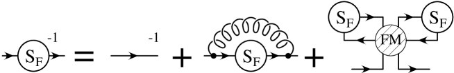
Figure 1: The diagram for the SD equation.

Generally the quark propagator is parametrised by

$$S^{R}_{Fh}(q)=\frac{i}{{\rm\ooalign{\hfil$/$\hfil\crcr\hbox{$q$}}}A_{h}(q^{2})-B_{h}(q^{2})}$$ (26)

where the index $h$ denotes the flavor. After the Wick rotation, we obtain $A_{h}(-q_{E}^{2})\equiv 1$. Then the resulting SD equation reads

$$B_{q}(-s) = m_{q}+\frac{3C_{F}}{16\pi^{2}}\int_{0}^{\Lambda_{\rm UV}^{2}}dr\bar{g}^{2}(s,r)\frac{B_{q}(-r)}{r+B_{q}^{2}(-r)}\left\{\theta(r-s)+\frac{r}{s}\theta(s-r)\right\}$$ (27)

$${}-\frac{G_{D}N_{C}^{2}w(s)}{8\pi^{4}}\int_{0}^{\Lambda_{\rm UV}^{2}}drw(r)\frac{rB_{q}(-r)}{r+B_{q}^{2}(-r)}\int_{0}^{\Lambda_{\rm UV}^{2}}dlw(l)\frac{lB_{s}(-l)}{l+B_{s}^{2}(-l)},$$

$$B_{s}(-s) = m_{s}+\frac{3C_{F}}{16\pi^{2}}\int_{0}^{\Lambda_{\rm UV}^{2}}dr\bar{g}^{2}(s,r)\frac{B_{s}(-r)}{r+B_{s}^{2}(-r)}\left\{\theta(r-s)+\frac{r}{s}\theta(s-r)\right\}$$ (28)

$${}-\frac{G_{D}N_{C}^{2}w(s)}{8\pi^{4}}\int_{0}^{\Lambda_{\rm UV}^{2}}drw(r)\frac{rB_{q}(-r)}{r+B_{q}^{2}(-r)}\int_{0}^{\Lambda_{\rm UV}^{2}}dlw(l)\frac{lB_{q}(-l)}{l+B_{q}^{2}(-l)},$$

with $s\equiv q_{E}^{2}$. These integral equations are solvable numerically.

Since the improved ladder approximation (ILA) model reproduces the asymptotic behavior of QCD, the quark mass function can be renormalized so that the solution of the SD equation is matched with the QCD quark mass function in the aymptotic region. We renormalize the quark mass function properly in the manner described in Ref.[16]. The renormalization constants $Z_{m_{q}}$ and $Z_{m_{s}}$ defined by $m_{q}=Z^{-1}_{m_{q}}m_{qR}$ and $m_{s}=Z^{-1}_{m_{s}}m_{sR}$ are determind by the condition

$$\frac{\partial B_{q}(\mu^{2})}{\partial m_{qR}}\bigg{|}_{m_{qR}=0}=1\quad\mbox{and}\quad\frac{\partial B_{s}(\mu^{2})}{\partial m_{sR}}\bigg{|}_{m_{sR}=0}=1.$$ (29)

Note that the flavor mixing interaction (FMI) does not disturb the asymptotic behavior of the ILA model and QCD because of the Gaussian type weight function.

5 Bethe–Salpeter Equation

The homogeneous Bethe–Salpeter (BS) equation is derived by

$$\frac{\delta^{2}\Gamma[S_{F}]}{\delta S_{Fmn}(x,y)\delta S_{Fn^{\prime}m^{\prime}}(y^{\prime},x^{\prime})}\chi_{n^{\prime}m^{\prime}}(y^{\prime},x^{\prime};P_{B})=0$$ (30)

where

$$\chi_{n^{\prime}m^{\prime}}(y^{\prime},x^{\prime};P_{B})=\langle 0|T\psi_{n^{\prime}}(y^{\prime})\overline{\psi}_{m^{\prime}}(x^{\prime})|\mbox{\boldmath{$P$}}\rangle$$ (31)

denotes the BS amplitude. The normalization condition is $\langle\mbox{\boldmath{$P$}}_{B}|\mbox{\boldmath{$P$}}^{\prime}_{B}\rangle=(2\pi)^{3}2P_{B0}\delta^{3}(\mbox{\boldmath{$P$}}_{B}-\mbox{\boldmath{$P$}}^{\prime}_{B})$ and $P_{B}:=(\sqrt{M_{B}^{2}+\mbox{\boldmath{$P$}}_{B}^{2}},\mbox{\boldmath{$P$}}_{B})$ is the on-shell momentum of the meson. Introducing the regularized BS amplitude by

$$\chi^{R}_{nm}(q;P_{B}):=f(-q_{+}^{2})\chi_{nm}(q;P_{B})f(-q_{-}^{2}),$$ (32)

$$q_{+}:=q+\frac{P_{B}}{2},\quad q_{-}:=q-\frac{P_{B}}{2},$$ (33)

the BS equation in momentum space becomes

$${S^{R}_{F}}^{-1}_{nn_{1}}(q_{+})\chi^{R}_{n_{1}m_{1}}(q;P_{B}){S^{R}_{F}}^{-1}_{m_{1}m}(q_{-})$$ (34)

$$= -iC_{F}\int_{k}\frac{1}{f(-k_{+}^{2})f(-k_{-}^{2})}\bar{g}^{2}(q_{E}^{2},k_{E}^{2})iD^{\mu\nu}(q-k)(\gamma_{\mu}\chi^{R}(k;P_{B})\gamma_{\nu})_{nm}$$

$${}+2iG_{\rm D}\epsilon^{ghf^{\prime}}\epsilon^{fh^{\prime}g^{\prime}}\delta_{ji}\int_{p,k}\frac{1}{f(-p^{2})f(-k_{+}^{2})f(-k_{-}^{2})}w\left(-p^{2}-q^{2}-k^{2}-\frac{P^{2}_{B}}{2}\right)$$

$$\times{\rm tr}^{\rm(DC)}[S^{R}_{Fh^{\prime}h}(p)]\Big{\{}(\gamma_{5})_{ba}{\rm tr}^{\rm(DC)}[\gamma_{5}\chi^{R}_{g^{\prime}f^{\prime}}(k;P_{B})]+1_{ba}{\rm tr}^{\rm(DC)}[\chi^{R}_{g^{\prime}f^{\prime}}(k;P_{B})]\Big{\}}$$

which is shown diagramatically in Fig.2.

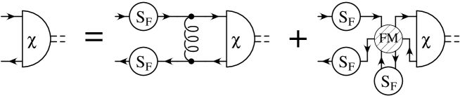
Figure 2: The diagram for the BS equation.

For the pseudoscalar state $|\mbox{\boldmath{$P$}}_{B}\rangle$, the last term in the braces does not contribute.

For the pion, the BS amplitude can be written in terms of four scalar amplitudes as in Ref.[16],

$$\chi^{R}_{nm}(k;P)=\delta_{ji}\frac{(\lambda^{\alpha})_{gf}}{2}\bigg{[}\bigg{(}\phi_{S}(k;P)+\phi_{P}(k;P){\rm\ooalign{\hfil$/$\hfil\crcr\hbox{$k$}}}+\phi_{Q}(k;P){\rm\ooalign{\hfil$/$\hfil\crcr\hbox{$P$}}}$$ (48)

$$\quad{}+\frac{1}{2}\phi_{T}(k;P)({\rm\ooalign{\hfil$/$\hfil\crcr\hbox{$P$}}}{\rm\ooalign{\hfil$/$\hfil\crcr\hbox{$k$}}}-{\rm\ooalign{\hfil$/$\hfil\crcr\hbox{$k$}}}{\rm\ooalign{\hfil$/$\hfil\crcr\hbox{$P$}}})\bigg{)}\gamma_{5}\bigg{]}_{ba}$$

where $\lambda^{\alpha}$ denotes the flavor structure of the pion state. For example, the neutral pion is given by $\alpha=3$

$$\lambda^{3}=\pmatrix{1&0&0\cr 0&-1&0\cr 0&0&0}.$$ (49)

On the other hand, for the $\eta$ and $\eta^{\prime}$ mesons, the BS amplitudes are written in terms of eight scalar amplitudes,

$$\chi^{R}_{nm}(k;P)=\delta_{ji}\frac{(\lambda^{qq})_{gf}}{2}\bigg{[}\bigg{(}\phi^{qq}_{S}(k;P)+\phi^{qq}_{P}(k;P){\rm\ooalign{\hfil$/$\hfil\crcr\hbox{$k$}}}+\phi^{qq}_{Q}(k;P){\rm\ooalign{\hfil$/$\hfil\crcr\hbox{$P$}}}$$ (77)

$$\quad{}+\frac{1}{2}\phi^{qq}_{T}(k;P)({\rm\ooalign{\hfil$/$\hfil\crcr\hbox{$P$}}}{\rm\ooalign{\hfil$/$\hfil\crcr\hbox{$k$}}}-{\rm\ooalign{\hfil$/$\hfil\crcr\hbox{$k$}}}{\rm\ooalign{\hfil$/$\hfil\crcr\hbox{$P$}}})\bigg{)}\gamma_{5}\bigg{]}_{ba}$$

$${}+\delta_{ji}\frac{(\lambda^{ss})_{gf}}{2}\bigg{[}\bigg{(}\phi^{ss}_{S}(k;P)+\phi^{ss}_{P}(k;P){\rm\ooalign{\hfil$/$\hfil\crcr\hbox{$k$}}}+\phi^{ss}_{Q}(k;P){\rm\ooalign{\hfil$/$\hfil\crcr\hbox{$P$}}}$$

$$\quad{}+\frac{1}{2}\phi^{ss}_{T}(k;P)({\rm\ooalign{\hfil$/$\hfil\crcr\hbox{$P$}}}{\rm\ooalign{\hfil$/$\hfil\crcr\hbox{$k$}}}-{\rm\ooalign{\hfil$/$\hfil\crcr\hbox{$k$}}}{\rm\ooalign{\hfil$/$\hfil\crcr\hbox{$P$}}})\bigg{)}\gamma_{5}\bigg{]}_{ba}$$

where the flavor matrices $\lambda^{qq},\lambda^{ss}$ are defined by

$$\lambda^{qq}=\pmatrix{1&0&0\cr 0&1&0\cr 0&0&0},\quad\lambda^{ss}=\pmatrix{0&0&0\cr 0&0&0\cr 0&0&\sqrt{2}}.$$ (78)

This is because the $qq$ and $ss$ components of the BS amplitude are mixed through the last term of the right hand side in Eq.$(\ref{AEQ:H110209:3})$ which is FMI. The BS equations for the $\eta$ and $\eta^{\prime}$ mesons are same. The ground state solution is identified with the $\eta$ meson and the first excited state solution is identified with the $\eta^{\prime}$ meson. Substituting Eq.$(\ref{AEQ:H110209:5})$ or Eq.$(\ref{AEQ:H110209:6})$ into Eq.$(\ref{AEQ:H110209:3})$, we obtain the coupled integral equations. The explicit form is rather complicated and we do not show it. Formally the equations can be written as

$$\phi_{\cal A}(q;P_{B})=\int_{k}M_{\cal AB}(q,k;P_{B})\phi_{B}(k;P_{B}).$$ (79)

$\phi_{A}$ or $\phi_{B}$ denotes the set of amplitudes, $\phi_{S},\phi_{P},\phi_{Q},\phi_{T}$ for the pion and $\phi^{qq}_{S},\phi^{qq}_{P},\phi^{qq}_{Q},\phi^{qq}_{T}$, $\phi^{ss}_{S},\phi^{ss}_{P},\phi^{ss}_{Q},\phi^{ss}_{T}$ for the $\eta$ and $\eta^{\prime}$ meson. Instead of solving Eq.$(\ref{AEQ:H110209:9})$ directly, we solve an eigenvalue problem

$$\lambda\phi_{\cal A}(q;P_{B})=\int_{k}M_{\cal AB}(q,k;P_{B})\phi_{B}(k;P_{B})$$ (80)

for a fixed $P_{B}^{2}=M_{B}^{2}=-P_{BE}^{2}=-M_{E}^{2}<0$. Then we plot and extrapolate the eigenvalue $\lambda$ as a function of $P_{B}^{2}$ and search for the on-shell point $\lambda=1$.

6 Decay Constant

To obtain the decay constant, we need the normalization of the BS amplitude which is derived from the inhomogeneous BS equation. In Ref.[16] the normalization condition in the momentum space is given by

$$\lim_{P\to P_{B}}i\int_{q\in I}\chi^{R}_{n_{1}m_{1}}(q;P_{B})\overline{\chi}^{R}_{m_{2}n_{2}}(q;P_{B})\frac{P^{\mu}}{-2P^{2}}\frac{\partial}{\partial P^{\mu}}\left[S^{R-1}_{Fn_{2}n_{1}}(q+\frac{P}{2})S^{R-1}_{Fm_{1}m_{2}}(q-\frac{P}{2})\right]=1$$ (81)

where the integral region is

$$I=\{q\,|\,{-(q\pm P_{B})^{2}}\leq\Lambda_{\rm UV}^{2}\}.$$ (82)

Using the normalized BS amplitude, the decay constant is obtained by

$$f_{B}=\lim_{P\to P_{B}}\frac{1}{P^{2}}\int_{q}\frac{1}{f(-q^{2}_{-})f(-q^{2}_{+})}{\rm tr}\bigg{[}\overline{\chi}^{R}(q;P_{B})i\gamma_{5}\frac{\lambda^{\alpha}}{2}\bigg{\{}\frac{f(-q^{2}_{-})+f(-q_{+}^{2})}{2}{\rm\ooalign{\hfil$/$\hfil\crcr\hbox{$P$}}}$$ (89)

$$+(-f(-q^{2}_{-})+f(-q^{2}_{+})){\rm\ooalign{\hfil$/$\hfil\crcr\hbox{$q$}}}\bigg{\}}\bigg{]}$$

$${}+\lim_{P\to P_{B}}\frac{1}{P^{2}}\int_{q}\frac{1}{f(-q^{2}_{-})f(-q^{2}_{+})}\left\{{\rm tr}[\overline{\chi}^{R}(q;P)(E^{\alpha}(q;P)+F^{\alpha}(q;P))]\right\}$$

where

$$E_{mn}^{\alpha}(q;P) := \int_{k}\frac{1}{f(-k^{2})}\left[\quad\left\{{\cal K}^{n^{\prime}n,mm^{\prime}}\left(-k,q-\frac{P}{2};-q-\frac{P}{2},k+P\right)\right.\right.$$ (90)

$$\quad\quad\quad-\left.{\cal K}^{n^{\prime}n,mm^{\prime}}\left(-k,q-\frac{P}{2};-q+\frac{P}{2},k\right)\right\}\left(i\gamma_{5}\frac{\lambda^{\alpha}}{2}S^{R}_{F}(k)\right)_{m^{\prime}n^{\prime}}$$

$$\quad\quad+\left\{{\cal K}^{n^{\prime}n,mm^{\prime}}\left(-k+P,q-\frac{P}{2};-q-\frac{P}{2},k\right)\right.$$

$$\quad\quad\quad-\left.\left.{\cal K}^{n^{\prime}n,mm^{\prime}}\left(-k,q+\frac{P}{2};-q-\frac{P}{2},k\right)\right\}\left(S_{F}^{R}(k)i\gamma_{5}\frac{\lambda^{\alpha}}{2}\right)_{m^{\prime}n^{\prime}}\right]$$

$$F_{mn}^{\alpha}(q;P) := 2G_{D}(\gamma_{5})_{ab}\delta_{ij}\int_{k,l}\frac{1}{f(-k^{2})f(-l^{2})}{\rm tr}^{\rm(DC)}[S^{R}_{Fg_{2}f_{2}}(k)]$$ (91)

$$\times\bigg{[}\bigg{\{}w\Big{(}-(q-\frac{P}{2})^{2}-k^{2}-l^{2}\Big{)}-w\Big{(}-q^{2}-\frac{3}{4}P^{2}-k^{2}-l^{2}+Pl\Big{)}\bigg{\}}$$

$${}\quad\times\epsilon^{ff_{2}f_{3}}\epsilon^{gg_{2}g_{3}}{\rm tr}^{\rm(DC)}[(S_{F}^{R}i\frac{\lambda^{\alpha}}{2})_{g_{3}f_{3}}(l)]$$

$${}+\bigg{\{}w\Big{(}-(q+\frac{P}{2})^{2}-k^{2}-l^{2}\Big{)}-w\Big{(}-q^{2}-\frac{3}{4}P^{2}-k^{2}-l^{2}-Pl\Big{)}\bigg{\}}$$

$${}\quad\times\epsilon^{ff_{2}f_{3}}\epsilon^{gg_{2}g_{3}}{\rm tr}^{\rm(DC)}[(i\frac{\lambda^{\alpha}}{2}S_{F}^{R})_{g_{3}f_{3}}(l)]\bigg{]}.$$

The term given in terms of $E^{\alpha}(q;P)$ and $F^{\alpha}(q;P)$ represents the correction to the Noether axialvector current due to the momentum dependencies of the effective lagrangian. For the pion, we can choose the flavor structure matrix $\lambda^{\alpha}$ of the Noether current in the above formula to match that of the BS amplitude. Then we obtain the decay constant $f_{\pi}$ in the usual sense. On the other hand, for the $\eta$ or $\eta^{\prime}$ mesons, the flavor structure of the BS amplitude depends on the relative and total momenta in general. Therefore we can not fix $\lambda^{\alpha}$ from the flavor structure of the BS amplitude. Instead we only consider the decay constants associated with the octet ($\alpha=8$) and singlet ($\alpha=0$) axialvector currents for the $\eta$ or $\eta^{\prime}$mesons, i.e., $f_{8}^{\eta}$, $f_{0}^{\eta}$, $f_{8}^{\eta^{\prime}}$ and $f_{0}^{\eta^{\prime}}$. The fact that the flavor structure of the $\eta$-$\eta^{\prime}$ meson BS amplitudes depend on the relative and total momenta means that one cannot define the $\eta$-$\eta^{\prime}$ mixing angle. It can be defined only in the limit of neglecting these momentum dependences.

7 Nambu–Goldstone Solution

A remark is given here about the Nambu–Goldstone solution. In the chiral limit, the effective action is invariant under the $SU_{L}(3)\times SU_{R}(3)\times U_{V}(1)$ transformation. Under the dynamical breakdown of this symmetry to $SU_{V}(3)\times U_{V}(1)$, we expect eight Nambu–Goldstone (NG) solutions. This can be proved by the same procedure as in Ref.[23]. However, we show here the existence of these NG solutions directly from the SD equation $(\ref{AEQ:H091214:2})$ and the BS equation $(\ref{AEQ:H110209:3})$. Multiplying the $\gamma_{5}\lambda^{\alpha}/2$ from left and $\gamma_{5}\lambda^{\alpha}/2$ from right to Eq.$(\ref{AEQ:H091214:2})$, we obtain

$$\{i\gamma_{5}\frac{\lambda^{\alpha}}{2},S_{F}^{R-1}(q)\}_{nm}-\{i\gamma_{5}\frac{\lambda^{\alpha}}{2},S_{0}^{R-1}(q)\}_{nm}$$ (92)

$$= -\frac{iC_{F}}{f(-q^{2})}\int_{p}\frac{1}{f(-p^{2})}\bar{g}^{2}(q_{E}^{2},p_{E}^{2})iD^{\mu\nu}(p-q)\left(\gamma_{\mu}\{S_{F}^{R}(p),i\gamma_{5}\frac{\lambda^{\alpha}}{2}\}\gamma_{\nu}\right)_{nm}$$

$${}+G_{D}\delta_{ji}\delta_{ba}\left(\frac{(\lambda^{\alpha})_{gg^{\prime}}}{2}\epsilon^{g^{\prime}f_{1}f_{2}}\epsilon^{fg_{1}g_{2}}+\epsilon^{gf_{1}f_{2}}\epsilon^{f^{\prime}g_{1}g_{2}}\frac{(\lambda^{\alpha})_{f^{\prime}f}}{2}\right)$$

$${}\times\int_{p,k}\frac{1}{f(-p^{2})f(-k^{2})}w(-q^{2}-p^{2}-k^{2}){\rm tr}^{\rm(DC)}[S^{R}_{Fg_{1}f_{1}}(p)]{\rm tr}^{\rm(DC)}[S^{R}_{Fg_{2}f_{2}}(k)].$$

In the chiral limit the second term of the left hand side vanishes. Furthermore if $\lambda^{\alpha}$ is an octet matrix i.e. ${\rm tr}[\lambda^{\alpha}]=0$, then a relation

$$\left(\frac{(\lambda^{\alpha})_{gg^{\prime}}}{2}\epsilon^{g^{\prime}f_{1}f_{2}}\epsilon^{fg_{1}g_{2}}+\epsilon^{gf_{1}f_{2}}\epsilon^{f^{\prime}g_{1}g_{2}}\frac{(\lambda^{\alpha})_{f^{\prime}f}}{2}\right)\delta_{g_{1}f_{1}}\delta_{g_{2}f_{2}}$$ (93)

$$= -4\epsilon^{gf_{1}f_{2}}\epsilon^{fg_{1}g_{2}}\delta_{g_{1}f_{1}}\frac{(\lambda^{\alpha})_{g_{2}f_{2}}}{2}$$

leads us to

$$\{i\gamma_{5}\frac{\lambda^{\alpha}}{2},S_{F}^{R-1}(q)\}_{nm}$$ (94)

$$= -\frac{iC_{F}}{f(-q^{2})}\int_{p}\frac{1}{f(-p^{2})}\bar{g}^{2}(q_{E}^{2},p_{E}^{2})iD^{\mu\nu}(p-q)\left(\gamma_{\mu}\{S_{F}^{R}(p),i\gamma_{5}\frac{\lambda^{\alpha}}{2}\}\gamma_{\nu}\right)_{nm}$$

$${}+2iG_{D}\delta_{ji}\delta_{ba}\epsilon^{gf_{1}f_{2}}\epsilon^{fg_{1}g_{2}}\int_{p,k}\frac{1}{f(-p^{2})f(-k^{2})}w(-q^{2}-p^{2}-k^{2})$$

$${}\times{\rm tr}^{\rm(DC)}[S^{R}_{Fg_{1}f_{1}}(p)]{\rm tr}^{\rm(DC)}[\gamma_{5}\{i\gamma_{5}\frac{\lambda^{\alpha}}{2},S^{R}_{F}(k)\}_{g_{2}f_{2}}].$$

Comparing this with Eq.$(\ref{AEQ:H110209:3})$, we obtain the Nambu–Goldstone solution for $\alpha=1,\dots,8$

$$\chi^{R}_{nm}(q;P=0)=N\{i\gamma_{5}\frac{\lambda^{\alpha}}{2},f(-q^{2})S^{R}_{F}(q)\}$$ (95)

where $N$ is a normalization constant. It can be also shown that $N$ equals to $1/f_{B}$ where $f_{B}$ is a decay constant defined in the previous section in the framework of the present ladder like approximation. It should also be noted that Eq.$(\ref{AEQ:H110210:4})$ does not hold for a singlet $\lambda^{\alpha=0}$.

8 Anomalous PCAC Relation

The matrix element of the PCAC relation $(\ref{AEQ:H100126:3})$ between a meson state $\langle\mbox{\boldmath{$P$}}|\,$ and the vacuum $|0\rangle$ in the ladder like approximation becomes

$$-f_{B}^{\alpha}M_{B}^{2}=2[m_{0}{\cal E}_{B}^{\alpha}]+\delta^{\alpha 0}{\cal A}_{B}$$ (96)

where $f_{B}^{\alpha}$ is the decay constant $f_{\pi},f_{8}^{\eta},f_{0}^{\eta},f_{8}^{\eta^{\prime}}$ or $f_{0}^{\eta^{\prime}}$. $[m_{0}{\cal E}_{B}^{\alpha}]$ and ${\cal A}_{B}$ are defined by

$$[m_{0}{\cal E}_{B}^{\alpha}]:=\lim_{P\to P_{B}}i\int_{q}\frac{f(-q_{-}^{2})+f(-q_{+}^{2})}{2f(-q_{-}^{2})f(-q_{+}^{2})}{\rm tr}[\overline{\chi}^{R}(q;P)m_{0}\gamma_{5}\frac{\lambda^{\alpha}}{2}],$$ (97)

$${\cal A}_{B}:=\lim_{P\to P_{B}}\int_{q}\frac{1}{f(-q_{+}^{2})f(-q_{-}^{2})}{\rm tr}[\overline{\chi}^{R}(q;P_{B})A(q;P)],$$ (98)

$$A_{mn}(q;P):=-3G_{D}(\gamma_{5})_{ab}\delta_{ij}\int_{k,l}\frac{1}{f(-k^{2})f(-l^{2})}{\rm tr}^{\rm(DC)}[S^{R}_{Fg_{2}f_{2}}(k)]$$ (99)

$$\times\bigg{[}w\Big{(}-(q-\frac{P}{2})^{2}-k^{2}-l^{2}\Big{)}\epsilon^{ff_{2}f_{3}}\epsilon^{gg_{2}g_{3}}{\rm tr}^{\rm(DC)}[(S^{R}_{F}i\frac{\lambda^{\alpha}}{2})_{g_{3}f_{3}}(l)]$$

$${}+w\Big{(}-(q+\frac{P}{2})^{2}-k^{2}-l^{2}\Big{)}\epsilon^{ff_{2}f_{3}}\epsilon^{gg_{2}g_{3}}{\rm tr}^{\rm(DC)}[(i\frac{\lambda^{\alpha}}{2}S^{R}_{F})_{g_{3}f_{3}}(l)]\bigg{]}$$

respectively. This relation is obtained systematically using the method of Sec.3 in Ref.[23]. Of course, we can also obtain this relation (96) directly from the SD equation $(\ref{AEQ:H091214:2})$ and the BS equation $(\ref{AEQ:H110209:3})$. If we employ the BS amplitude in the chiral limit like Eq.(95), it holds that

$$[m_{0}{\cal E}_{B}^{\alpha}]=m_{q}\langle\bar{q}q\rangle_{0}/f_{B}=m_{qR}\langle\bar{q}q\rangle_{R}/f_{B}.$$ (100)

Eq.(96) with Eq.(100) leads us to the Gell-Mann, Oakes and Renner mass formula

$$M_{B}^{2}f_{B}^{2}\simeq-2m_{q}\langle\bar{q}q\rangle\quad\mbox{for}\quad\alpha\neq 0.$$ (101)

For later use, we define the ratio

$${\cal R}_{\alpha}(P_{E}^{2})=\frac{f_{B}^{\alpha}(P_{E}^{2})P_{E}^{2}}{2[m_{0}{\cal E}^{\alpha}_{B}(P_{E}^{2})]+\delta^{\alpha 0}{\cal A}_{B}(P_{E}^{2})},$$ (102)

which is to be unity at the on-mass-shell point of the Bethe-Salpeter solution. This condition is useful in checking the numerical extrapolation procedure.

9 Numerical Results

In the present model, there are seven input parameters. Five of them are the parameters of the improved ladder approximation (ILA) model of QCD: the current quark mass $m_{qR}$ for the up and down quarks, the scale parameter of QCD $\Lambda_{\rm QCD}$, the infrared cut-off $t_{\rm IF}$ for the running coupling constant, the smoothness parameter $t_{0}$ and the ultraviolet cut-off $\Lambda_{\rm UV}$. We take the value of $t_{0}$ from the result of Ref.[13], namely, $t_{0}=-3$. As explained there this smoothness parameter $t_{0}$ is introduced just for the stability of the numerical calculations and has no physical meanings. We take $\Lambda_{\rm UV}=100$ [GeV] because the physical observables depend on it rather weakly after the renormalization as far as we use a reasonably large value of $\Lambda_{\rm UV}$. The renormalization point $\mu$ is taken as $\mu=2$ [GeV]. The infrared cut-off $t_{\rm IF}$ controls the strength of the running coupling constant in the low $q^{2}_{E}$ region. Therefore its value is directly related to the size of the dynamical chiral symmetry breaking. We take $t_{\rm IF}=-0.5$. In the case of no FMI, $t_{\rm IF}=-0.5$ gives $-\langle\bar{\psi}\psi\rangle^{1/3}_{R}=259$ [MeV] with $\Lambda_{\rm QCD}=600$ [MeV] in the chiral limit.

We choose $\Lambda_{\rm QCD}=600$ [MeV]. Although this value is somewhat larger than the “standard” value $\Lambda_{\rm QCD}=100\sim 300$ [MeV], it is necessary for the rainbow gluon self energy to generate the dynamical chiral symmetry breaking strongly[13, 16]. Of course if the dynamical chiral symmetry breaking is caused by the flavor mixing interaction mainly, we may choose a smaller $\Lambda_{\rm QCD}$. But in such a situation, a careful analysis is necessary. Since the phase transition is of the first order, there may exist multiple SD solutions. We will report such results elsewhere [24]. Therefore in this paper we concentrate only on the case that the chiral symmetry breaking is generated mainly by the gluon exchange interaction.

We have two new parameters associated with the flavor mixing interaction (FMI), i.e., $G_{D}$ and $\kappa$. Instead of $G_{D}$, we use the parameter $I_{G}$ defined by

$$G_{D}\,\mbox{[GeV${}^{-5}$]}\,=:-(I_{G}\,\mbox{[GeV${}^{-1}$]})^{5}.$$ (103)

This parameter is chosen freely so that we study the effects of the $U_{A}(1)$ anomaly on the $\eta$-$\eta^{\prime}$ system. The $\kappa$ parameter is taken as

$$\kappa=0.7\,\mbox{[GeV${}^{-2}$]}.$$ (104)

This value corresponds to the form factor of the instanton of the average size $\rho$, about $1/3$ [fm]. The instanton form factor,

$$\frac{1}{x_{E}^{2}+\rho^{2}}\propto 1-\frac{x_{E}^{2}}{\rho^{2}}+\cdots$$ (105)

can be identified with the Fourier transformation of the weight function

$${\rm F.T.}\,w(q_{E}^{2})=C\exp\left(-\frac{x_{E}^{2}}{4\kappa}\right)\propto 1-\frac{x_{E}^{2}}{4\kappa}+\cdots$$ (106)

with

$$4\kappa=\rho^{2}.$$ (107)

The values of the model parameters we use throughout this article are $\Lambda_{\rm UV}=100$ [GeV], $\Lambda_{\rm QCD}=600$ [MeV], $t_{0}=-3$, $t_{\rm IF}=-0.5$, $\mu=2$ [GeV] and $\kappa=0.7$ [GeV^-2].

Let us now discuss the solutions of the SD equation. Our numerical results are shown in Table 1 and Figs.3 and 4. As can be seen from them, the chiral symmetry breaking is induced mainly by the gluon exchange interaction, and the effect of FMI to the chiral quark condensate seems very small. When $I_{G}$ increases from zero to 2.4, $B_{q}(0)$ increases only 4-6%, and $\langle\bar{q}q\rangle_{R}$ changes by about 10 to 20 %. One may wonder whether the range of variation is too small for its effects to be seen, but, as we will see later, this $I_{G}$ gives a large mass to $\eta$ and $\eta^{\prime}$. Since the perturbative quark mass contribution to the quark condensate is subtracted in our definition, the absolute value of $\langle\bar{s}s\rangle_{R}$ is smaller than that of $\langle\bar{q}q\rangle_{R}$ ($q=u,d$). Our results in $m_{qR}=5$ [MeV] and $m_{sR}=100$ [MeV] are $\langle\bar{s}s\rangle_{R}/\langle\bar{q}q\rangle_{R}=0.85$ and 0.63 for $I_{G}=0$ and 2.4 [GeV^-1] respectively. These are in reasonable agreement with the QCD sum rule results: $\langle\bar{s}s\rangle_{R}/\langle\bar{u}u\rangle_{R}=0.8\pm 0.1$ [25] and $\langle\bar{s}s\rangle_{R}/\langle\bar{u}u\rangle_{R}=0.6\pm 0.1$ [26]. The absolute value of the u,d-quark condensate increases as $I_{G}$ increases, while that of the s-quark condensate decreases as $I_{G}$ increases. It is an interesting feature in the present model. In the case of the Nambu-Jona-Lasinio (NJL) model with FMI, both condensates increase. We do not find out the intuitive explanation of the difference of this behavior between the NJL model and the present model.

Figure 3: $q_{E}^{2}$ dependences of the solutions of the SD equation in the $SU(3)$ chiral limit with $I_{G}=0.0,1.6,2.0,2.4$ [GeV^-1].

Figure 4: $q_{E}^{2}$ dependences of the solutions of the SD equation in the $SU(2)$ chiral limit with $m_{sR}=100$ [MeV] and $I_{G}=0.0,1.6,2.0,2.4$ [GeV^-1].

$m_{qR}$[MeV]	$m_{sR}$[MeV]	$I_{G}$[GeV-1]	$B_{q}(0)$	$B_{s}(0)$	$\langle\bar{q}q\rangle_{R}$[GeV3]	$\langle\bar{s}s\rangle_{R}$ [GeV3]
0	0	0.0	$1.10$	$1.10$	$-(0.259)^{3}$	$-(0.259)^{3}$
0	0	1.6	$1.11$	$1.11$	$-(0.260)^{3}$	$-(0.260)^{3}$
0	0	2.0	$1.11$	$1.11$	$-(0.262)^{3}$	$-(0.262)^{3}$
0	0	2.4	$1.14$	$1.14$	$-(0.268)^{3}$	$-(0.268)^{3}$
0	100	0.0	$1.10$	$1.22$	$-(0.259)^{3}$	$-(0.245)^{3}$
0	100	1.6	$1.11$	$1.22$	$-(0.261)^{3}$	$-(0.244)^{3}$
0	100	2.0	$1.12$	$1.22$	$-(0.266)^{3}$	$-(0.241)^{3}$
0	100	2.4	$1.16$	$1.24$	$-(0.276)^{3}$	$-(0.235)^{3}$
5	100	0.0	$1.11$	$1.22$	$-(0.259)^{3}$	$-(0.245)^{3}$
5	100	1.6	$1.11$	$1.22$	$-(0.261)^{3}$	$-(0.244)^{3}$
5	100	2.0	$1.13$	$1.23$	$-(0.266)^{3}$	$-(0.241)^{3}$
5	100	2.4	$1.17$	$1.24$	$-(0.276)^{3}$	$-(0.236)^{3}$

Table 1: Dependences of the solutions of the SD equations at $q_{E}^{2}=0$ and the quark condensates on the strength of FMI with three sets of the quark masses, (i) $m_{qR}=m_{sR}=0$, (ii) $m_{qR}=0$, $m_{sR}=100$ [MeV] and (iii) $m_{qR}=5$ [MeV], $m_{sR}=100$ [MeV]. Here q represents the u and d quarks.

Let us now turn to the discussion of the solutions of the BS equation. Our numerical results for the pion are summarized in Table 2. Here we have not performed the precise parameter fittings so as to reproduce the observed pion mass and decay constant since solving the BS equation of the non-local interaction requires the rather large computer resouces. We observe that the pion mass and decay constant are not sensitive to the flavor mixing interaction. The deviation of the slope $M_{\pi}^{2}/m_{qR}$ from the slope $-2\langle\bar{q}q\rangle_{R}/f_{\pi}^{2}$ derived from Gell-Mann-Oakes-Renner (GMOR) relation is about 16% at $m_{qR}=5$ [MeV] and $I_{G}=2.4$ [GeV^-1]. We consider this amount of the deviation of the GMOR relation may come from the Euclid $\to$ Minkowski extrapolation, since the ratio ${\cal R}$ defined in Eq.(102) deviates from unity by 5%, which indicates the size of the numerical error for $M_{\pi}^{2}$ and $f_{\pi}$ in the extrapolation procedure.

$m_{qR}$[MeV]	$m_{sR}$[MeV]	$I_{G}$[GeV-1]	$M_{\pi}$[MeV]	$f_{\pi}$[MeV]	${\cal R}$
0	0	$0.0$	$0$	$86$	—
0	0	$1.6$	$0$	$87$	—
0	0	$2.0$	$0$	$89$	—
0	0	$2.4$	$0$	$95$	—
0	100	$0.0$	$0$	$86$	—
0	100	$1.6$	$0$	$88$	—
0	100	$2.0$	$0$	$91$	—
0	100	$2.4$	$0$	$101$	—
5	100	$0.0$	$159$	$88$	$1.06$
5	100	$1.6$	$158$	$90$	$1.06$
5	100	$2.0$	$157$	$94$	$1.05$
5	100	$2.4$	$152$	$103$	$1.05$

Table 2: Dependences of the solutions of the pion BS equation on the strength of FMI with three sets of the quark masses, (i) $m_{qR}=m_{sR}=0$, (ii) $m_{qR}=0$, $m_{sR}=100$ [MeV] and (iii) $m_{qR}=5$ [MeV], $m_{sR}=100$ [MeV].

The BS solutions for the $\eta$ and $\eta^{\prime}$ mesons are given in Tables 3 and 4. Since the BS equation is homogeneous, the absolute sign of the BS amplitudes, and therefore the decay constants, cannot be determined. We choose the sign of $f_{8}$ ($f_{0}$) to be positive for $\eta$ ($\eta^{\prime}$). The masses of $\eta$ and $\eta^{\prime}$ and their decay constants depend strongly on the flavor mixing interaction. Especially, the $\eta^{\prime}$ meson mass seems sensitive to the flavor mixing interaction. This is in contrast to the pion result. $U_{A}(1)$ symmetry breaking gives a large effect on the $\eta$ and $\eta^{\prime}$ sector.

In order to see the effects of the flavor mixing, we introduce the mixing angles for the $\eta$ and $\eta^{\prime}$ mesons,

$$\frac{-f_{0}^{\eta}}{f_{8}^{\eta}}=\tan\theta_{\eta},\quad\frac{f_{8}^{\eta^{\prime}}}{f_{0}^{\eta^{\prime}}}=\tan\theta_{\eta^{\prime}}.$$ (108)

The results are presented in Tables 3 and 4. Since the flavaor structure of the $\eta$-$\eta^{\prime}$ meson BS amplitudes depend on the relative and total momenta, the above definitions of the mixing angles are the kinds of the averaged quantities.

In the $SU(3)$ symmetry limit, no flavor mixing occurs and $\theta_{\eta}=\theta_{\eta^{\prime}}=0$. On the other hand, in the broken $SU(3)$ case without FMI, $\eta$ and $\eta^{\prime}$ are in the ideally mixed states, i.e., $\theta=\arctan(-\sqrt{2})=-54.7^{\circ}$. The mixing angles $\theta_{\eta}$ and $\theta_{\eta^{\prime}}$ increase as FMI becomes strong. In the case of $m_{qR}=5$ [MeV], $m_{sR}=100$ [MeV] and $I_{G}=2.4$ [GeV^-1], the reasonable values of the $M_{\eta}$ and $M_{\eta^{\prime}}$ are obtained, the calculated $M_{\eta}$ is 7% smaller than the observed $M_{\eta}$ and the calculated $M_{\eta^{\prime}}$ is 11% larger than the observed $M_{\eta^{\prime}}$. In this model parameters, the calculated mixing angle for the $\eta^{\prime}$ meson $\theta_{\eta^{\prime}}$ is more than 5/3 times of the calculated mixing angle for the $\eta$ meson $\theta_{\eta}$. It means that the momentum dependences of the flavor structures of the $\eta$ and $\eta^{\prime}$ mesons are not so small and the momentum independent treatment of the $\eta$-$\eta^{\prime}$ mixing angle is rather questionable.

The last column of Tables 2, 3 and 4 gives the ratio $\cal R$ in Eq.(102) for finite quark mass. As it should be $1$ at the on-mass-shell point identically, it is a good indicator of the ambiguity, or error, coming from the extrapolation from the Euclidean kinematics to the Minkowski on-mass-shell kinematics. Here we carry out the quadratic extrapolations of the eigenvalue $\lambda$ and the ratio $\cal R$ and the linear extrapolation of the decay constant $f$ from the Euclid region to the on-mass-shell point. In the case of the weak FMI, our extapolation procedure works rather well. The quality of the extrapolation can be seen in Fig.5. For heavier meson masses, ${\cal R}$ deviates from 1 significantly. This indicates an extrapolation error. In fact, for $M_{B}>700$ [MeV] the extrapolation becomes very difficult in the quadratic extrapolation. For instance, ${\cal R}_{0}^{\eta}$ for $I_{G}=2.4$ [GeV^-1] shown in Table 3 largely deviates from 1. Fig.6 shows the extrapolation in this case, where the lines of $\lambda$ and ${\cal R}_{8}^{\eta}$ are almost straight but the curve of ${\cal R}_{0}^{\eta}$ is not. This may be a reason why ${\cal R}_{0}^{\eta}$ deviates from unity. We have performed the extrapolation of ${\cal R}_{0}^{\eta}$ by using a rational function which is shown in Fig.6 by the dotted line and the result is improved well. As for the $\eta^{\prime}$ meson, the extrapolation of the eigenvalue, the rations ${\cal R}_{8}^{\eta^{\prime}}$ and ${\cal R}_{0}^{\eta^{\prime}}$ are shown in Fig.7.

From Table 4 one can see that in the chiral limit, $\eta^{\prime}$ state is a pure flavor singlet state and has finite mass. This mass is due to FMI and it means $\eta^{\prime}$ is not the Goldstone boson. One of the interesting question is that how much $\eta^{\prime}$ loses the the Goldstone boson nature. In the present range of the $U_{A}(1)$ breaking interaction strength, the flavor singlet pseudoscalar meson state has mass from 194 [MeV] to 634 [MeV]. On the other hand the decay constant changes only less than 8%. Further studies of the $\eta^{\prime}$ properties such as the decay amplitudes are necessary in order to understand the nature of the $\eta^{\prime}$ meson.

We plot the $\eta^{\prime}$ meson mass as a function of the $U_{A}(1)$ breaking parameter $I_{G}$ in Fig.8. The effect of the mixing of $u,d$ quark component seems to be negligible and the $\eta^{\prime}$ mass grows rapidly from $I_{G}\sim 2.0$ [GeV^-1].

$m_{qR}$	$m_{sR}$	$I_{G}$	$M_{\eta}$	$f_{8}^{\eta}$	$f_{0}^{\eta}$	$\theta_{\eta}$	${\cal R}_{8}^{\eta}$	${\cal R}_{0}^{\eta}$
[MeV]	[MeV]	[GeV-1]	[MeV]	[MeV]	[MeV]	[deg]
0	0	$0.0$	$0$	$86$	$0$	0	—	—
0	0	$1.6$	$0$	$87$	$0$	0	—	—
0	0	$2.0$	$0$	$89$	$0$	0	—	—
0	0	$2.4$	$0$	$95$	$0$	0	—	—
0	100	$0.0$	$0$	$50$	$70$	$-54.7$	—	—
0	100	$1.6$	$203$	$56$	$68$	$-50.5$	$1.03$	$1.04$
0	100	$2.0$	$351$	$71$	$58$	$-39.2$	$1.00$	$1.03$
0	100	$2.4$	$495$	$106$	$22$	$-11.7$	$1.00$	$0.62$ ($1.07$)
5	100	$0.0$	$159$	$51$	$72$	$-54.7$	1.05	1.05
5	100	$1.6$	$258$	$57$	$69$	$-50.4$	$1.02$	$1.03$
5	100	$2.0$	$387$	$75$	$58$	$-37.7$	$1.00$	$1.05$
5	100	$2.4$	$511$	$113$	$19$	$-9.5$	$1.01$	$0.55$ ($1.00$)

Table 3: Dependences of the $\eta$-meson solutions of the coupled channel BS equation on the strength of FMI with three sets of the quark masses, (i) $m_{qR}=m_{sR}=0$, (ii) $m_{qR}=0$, $m_{sR}=100$ [MeV] and (iii) $m_{qR}=5$ [MeV], $m_{sR}=100$ [MeV]. The values in the brace are obtained by the rational extrapolation.

$m_{qR}$	$m_{sR}$	$I_{G}$	$M_{\eta}$	$f_{8}^{\eta}$	$f_{0}^{\eta}$	$\theta_{\eta}$	${\cal R}_{8}^{\eta}$	${\cal R}_{0}^{\eta}$
[MeV]	[MeV]	[GeV-1]	[MeV]	[MeV]	[MeV]	[deg]
0	0	$0.0$	$0$	$0$	$86$	0	—	—
0	0	$1.6$	$194$	$0$	$87$	0	—	$1.04$
0	0	$2.0$	$350$	$0$	$88$	0	—	$1.02$
0	0	$2.4$	$634$	$0$	$94$	0	—	$1.06$
0	100	$0.0$	$723$	$-101$	$72$	$-54.7$	$1.05$	$1.05$
0	100	$1.6$	$731$	$-99$	$76$	$-52.5$	$1.05$	$1.07$
0	100	$2.0$	$764$	$-88$	$88$	$-45.0$	$1.06$	$1.10$
0	100	$2.4$	$1020$	$-41$	$118$	$-19.2$	$1.09$	$1.30$($1.32$)
5	100	$0.0$	$723$	$-101$	$72$	$-54.7$	$1.05$	$1.05$
5	100	$1.6$	$732$	$-98$	$77$	$-51.8$	$1.05$	$1.07$
5	100	$2.0$	$777$	$-86$	$90$	$-43.7$	$1.06$	$1.11$
5	100	$2.4$	$1060$	$-36$	$122$	$-16.4$	$1.09$	$1.33$

Table 4: Dependences of the $\eta^{\prime}$-meson solutions of the coupled channel BS equation on the strength of FMI with three sets of the quark masses, (i) $m_{qR}=m_{sR}=0$, (ii) $m_{qR}=0$, $m_{sR}=100$ [MeV] and (iii) $m_{qR}=5$ [MeV], $m_{sR}=100$ [MeV]. The value in the brace is obtained by the rational extrapolation.

Figure 5: Extrapolation of the eigenvalue and the ratios for the $\eta$ meson with $m_{qR}=0$, $m_{sR}=100$ [MeV] and $I_{G}=1.6$ [GeV^-1].

Figure 6: Extrapolation of the eigenvalue and the ratios for the $\eta$ meson with $m_{qR}=0$, $m_{sR}=100$ [MeV] and $I_{G}=2.4$ [GeV^-1].

Figure 7: Extrapolation of the eigenvalue and the ratios for the $\eta^{\prime}$ meson with $m_{qR}=0$, $m_{sR}=100$ [MeV] and $I_{G}=2.4$ [GeV^-1].

Figure 8: $I_{G}$ dependence of the mass of the $\eta^{\prime}$ meson with $m_{qR}=0$ and $m_{sR}=100$ [MeV].

The $\eta$-meson properties have been studied extensively in the three-flavor NJL model with the instanton induced $U_{A}(1)$ breaking flavor mixing interaction (FMI) in Ref.[11] and it has been shown that the $\eta$-meson mass, the $\eta\rightarrow\gamma\gamma$, $\eta\rightarrow\gamma$, $\mu^{-}\mu^{+}$ and $\eta\rightarrow\pi^{0}\gamma\gamma$ decay widths are reproduced well with the rather strong FMI. In this case the contribution from FMI to the dynamical mass of the up and down quarks is about 44% of that from the usual $U_{L}(3)\times U_{R}(3)$ invariant four-quark interaction. In contrast with it, the contribution from FMI to the dynamical quark mass is very small in the present study. To make the situation clear, let us compare the strength of FMI in the present case with that in the NJL model case. The naive way is to compare the following two quantities,

$$\int_{0}^{\infty}dqe^{-\kappa q^{2}}I_{G}^{5},$$ (109)

in the present model and

$$\int_{0}^{\Lambda}dq\frac{16\pi^{4}}{9\Lambda^{5}}G_{D}^{\rm eff},$$ (110)

in the NJL model. In this manner $I_{G}=2.4$ [GeV^-1] corresponds to $G_{D}^{\rm eff}=0.73$, which is rather close to the value determined in Ref.[11], $G_{D}^{\rm eff}=0.7$. It means the strength of FMI is almost same in the both cases. It is not clear why the contribution from FMI to the dynamical quark mass is so different in the two cases.

It should be noted here that as can be seen from Fig.2, FMI operates on the pseudoscalar meson states as the effective 4-quark interaction reduced by contracting a quark-antiquark pair into a quark condensate. Therefore the effective strength of FMI is not $G_{D}$ but $G_{D}\langle\bar{q}q\rangle$. In our present model parameters, the dynamical chiral symmetry breaking is mostly driven by the one-gluon exchange type interaction. If one reduces the strength of the one-gluon type interaction in the infrared region, the quark condensate becomes smaller and the effective strength of FMI on the meson states becomes weaker. Therefore there is a possibility of taking rather strong FMI without destroying the success of the present description of the $\eta$ and $\eta^{\prime}$ meson masses. In the case where FMI is dominant in the infrared region, we expect that the chiral phase transition becomes the first order and there may exist multiple solutions of the SD equation. In such a situation, more careful analyses are required, which will be reported elsewhere [24].

10 Summary and Conclusions

The improved ladder approximation of QCD has successfully described the low-energy properties of QCD [13, 14, 16]. In this article, we have studied the $\eta$ and $\eta^{\prime}$ mesons in this approach. It is expected that the $U_{A}(1)$ anomaly plays an important role in the $\eta$ and $\eta^{\prime}$ mesons and therefore we have introduced the instanton induced $U_{A}(1)$ breaking 6-quark determinant interaction [22, 7] in the improved ladder approximation model of QCD. We have derived the Schwinger-Dyson (SD) equations for the light quark propagators and the Bethe-Salpeter (BS) equations for the pion, $\eta$ and $\eta^{\prime}$ in the lowest order (rainbow-ladder) approximation using the Cornwall-Jackiw-Tomboulis (CJT) effective action formulation [21].

Using the same model parameters of the running coupling constant used in [16], we have obtained reasonable values of $M_{\pi}$, $M_{\eta}$, $M_{\eta^{\prime}}$, $f_{\pi}$ and $\langle\bar{q}q\rangle_{R}$ with a relatively weak flavor mixing interaction (FMI), for which the chiral symmetry breaking is dominantly induced by the soft-gluon exchange interaction. It is in contrast with the Nambu-Jona-Lasinio (NJL) model results, where about 1/3 of the dynaminacl quark mass is due to FMI [11].

As far as we know, the $\eta^{\prime}$ BS equation which includes the running coupling aspect of QCD and the effect of the $U_{A}(1)$ anomaly has not been solved so far. In the case of the NJL model, the $\eta^{\prime}$ mass has unphysical large imaginary part associated with the unphysical decay channel $\eta^{\prime}\to\bar{q}q$. On the other hand, the present model predicts a bound $\eta^{\prime}$ although it may not perfectly confine quarks. The bound state is obtained as the quark mass function becomes rather large, $B(-q^{2}_{E})\sim 1$ [GeV] at $q_{E}=0$, in this model, while it is independent of the momentum in the NJL model.

Since the flavor structure of the $\eta$-$\eta^{\prime}$ meson BS amplitudes depend on the relative and total momenta, one cannot define the $\eta$-$\eta^{\prime}$ mixing angle unambiguously. It can be defined only in the limit of neglecting these momentum dependences and it should be examined whether such an approximation is reasonable. Our numerical results indicate that the momentum independent treatment of the flavor mixing is rather questionable.

In the chiral limit we can define the $\eta_{0}$ decay constant $f_{0}$ without any ambiguity. (Here $\eta_{0}$ means the pure flavor singlet state.) Our numerical results show that $(|f_{0}|-f_{\pi})/f_{\pi}\leq 0.012$ in our parameter range though $M_{\eta_{0}}$ changes from 194 [MeV] to 634 [MeV]. There is no low-energy theorem for the $\eta_{0}$ decay constant $f_{0}$ since the $U_{A}(1)$ symmetry is explicitly broken by the anomaly. Therefore the present result of $f_{0}$ should contain the information of the low-energy dynamics of QCD.

The present result is our first step towards quantitative understanding of the flavor mixing interaction. With the BS solutions in hand, we may calculate static properties and decay amplitudes of $\eta$ and $\eta^{\prime}$. Our model is regarded as a low energy effective theory, which is consistent with chiral symmetry, its spontaneous breakdown and the $U_{A}(1)$ anomaly. It should be stressed that the approximation used in solving and renormalizing the amplitudes also respect these symmetry properties. Thus our approach is suitable for further studies of the $\eta$ and $\eta^{\prime}$ systems, which are desirable in order to clarify the role of the $U_{A}(1)$ anomaly in the low-energy QCD.

References

• [1] S. Weinberg, Phys. Rev. D11 (1975) 3583.
• [2] G. ’t Hooft, Nucl. Phys. B72 (1974) 461.
• [3] For a review, G.A. Christos, Phys. Rep. 116 (1984) 251.
• [4] P. Di Vecchia and G. Veneziano, Nucl. Phys. B171 (1980) 253; C. Rosenzweig, J. Schechter and T. Trahern, Phys. Rev. D21 (1980) 3388; E. Witten, Ann. Phys. (N.Y.) 128 (1980) 363.
• [5] H. Leutwyler, Phys. Lett. B374 (1996) 163; Nucl. Phys. Proc. Suppl. 64 (1998) 223; P. Herrera-SiklΓ³dy, J.I. Latorre, P.Pascual and J. Taron, Nucl. Phys. B497 (1997) 345.
• [6] G. ’t Hooft, Phys. Rep. 142 (1986) 357.
• [7] G. ’t Hooft, Phys. Rev. D14 (1976) 3432.
• [8] For a review, T. SchΓ€fer and E.V. Shuryak, Rev. Mod. Phys. 70 (1998) 323, and references therein.
• [9] Y. Nambu and G. Jona-Lasinio, Phys. Rev, 122 (1961) 345; 124 (1961) 246.
• [10] T. Kunihiro and T. Hatsuda, Phys. Lett. B206 (1988) 385; T. Hatsuda and T. Kunihiro, Z. Phys. C51 (1991) 49; Phys. Rep. 247 (1994) 221; V. Bernard, R.L. Jaffe and U.-G. Meissner, Nucl. Phys.B308 (1988) 753; M. Takizawa, K. Tsushima, Y. Kohyama and K. Kubodera, Prog. Theor. Phys. 82 (1989) 481; Nucl. Phys. A507 (1990) 611; H. Reinhardt and R. Alkofer, Phys. Lett. B207 (1988) 482; R. Alkofer and H. Reinhardt, Z. Phys. C45 (1989) 275; S. Klimt, M. Lutz, U. Vogl and W. Weise, Nucl. Phys.A516 (1990) 429; U. Vogl, M. Lutz, S. Klimt and W. Weise, Prog. Part. Nucl. Phys. 27 (1991) 195.
• [11] M. Takizawa and M. Oka, Phys. Lett. B359 (1995) 210; B364 (1995) 249 (E); Y.Nemoto, M. Oka and M. Takizawa, Phys. Rev. D54 (1996) 6777; M. Takizawa, Y.Nemoto and M. Oka, Phys. Rev. D55 (1997) 4083.
• [12] K. Higashijima, Phys. Rev. D29 (1984) 1228; V.A. Miransky, Sov. J. Nucl. Phys. 38 (1984) 280.
• [13] K. Aoki, M. Bando, T. Kugo, M.G. Mitchard and H. Nakatani, Prog. Theor. Phys. 84(1990) 683.
• [14] K. Aoki, M. Bando, T. Kugo, M.G. Mitchard, Prog. Theor. Phys. 85 (1991) 355.
• [15] K. Aoki, T. Kugo, M.G. Mitchard, Phys. Lett. B266 (1991) 467.
• [16] K. Naito, K. Yoshida, Y. Nemoto, M. Oka and M. Takizawa, Phys. Rev. C 59 (1999) 1722. In this paper, $\overline{\chi}^{R}(q;P_{B})$ in Eqs.$(57)$ and $(60)$ should be replaced by $\overline{\chi}(q;P_{B})$.
• [17] For a review, C.D. Roberts and A.G. Williams, Prog. Part. Nucl. Phys. 33 (1994) 477, and references therein.
• [18] P. Jain and H.J. Munczek, Phys. Rev. D48 (1993) 5403.
• [19] D. Klabučar and D. Kekez, Phys. Rev. D48 (1998) 096003.
• [20] M.R. Frank and T. Meissner, Phys. Rev. C57 (1998) 345.
• [21] J.M. Cornwall, R. Jackiw and E. Tomboulis, Phys. Rev. D10 (1974) 2428.
• [22] M. Kobayashi and T. Maskawa, Prog. Theor. Phys. 44 (1970) 1422; M. Kobayashi, H. Kondo and T. Maskawa, Prog. Theor. Phys. 45 (1971) 1955.
• [23] K. Naito, K. Yoshida, Y. Nemoto, M. Oka and M. Takizawa, Phys. Rev. C 59 (1999) 1095.
• [24] K. Naito, M. Takizawa and M. Oka, in preparation.
• [25] L.J. Reinders, H. Rubinstein and S. Yazaki, Phys. Reports 127 (1985) 1.
• [26] S. Narison, Phys. Lett. B216 (1989 191.