New Higgs Signals from Flavor Physics
in Large Extra Dimensions

In a realistic theory with large extra dimensions and TeV scale gravity, there are often other particles living in the extra dimensions in addition to gravitons. A well motivated candidate is the flavon in a flavor theory which explains the smallness of the fermion masses by the large volume of the extra dimensions. The flavon interactions involve the Higgs field and can therefore give rise to new mechanisms of Higgs boson production. We study these new Higgs signals, including both real flavon emission and virtual flavon exchange. They could provide powerful probes of the string scale which are comparable to the extensively studied graviton production, if the flavons and the graviton feel the same number of extra dimensions. If the flavons only live in a subspace of the extra dimensions, they can yield even stronger bounds and may generate spectacular displaced vertex signals. Our study also applies to a four dimensional flavor theory with light flavons as well as to any theory with bulk scalar fields coupled to the Higgs and fermions.

Submitted to Nucl. Phys. B

1 Introduction

The Standard Model (SM) is very successful in explaining most precision data from current collider experiments, but still we have not found (or tested) all ingredients of the SM. The elusive Higgs particle is yet to be discovered, and its interactions with the SM fermions and gauge bosons will need to be measured before we close the final chapter in the quest for the correct theory of particle physics at the weak scale.

Given the success of the Standard Model, there are still several unresolved puzzles. An important one is related to flavor, i.e. the size of the fermion masses and the generation of the CKM matrix. In the Standard Model, the fermion masses arise from the Yukawa interactions between the fermions and the Higgs. We do not understand why all fermion Yukawa couplings other than the top Yukawa coupling are so small or why the CKM matrix is approximately diagonal. The smallness of the fermion Yukawa couplings also leads to the suppression of direct $s$-channel Higgs production, making the Higgs discovery a challenging task.

A natural explanation for the smallness of the fermion Yukawa couplings is that there is an enlarged (flavor) symmetry under which the direct couplings between the light fermions and the Higgs are forbidden in the symmetry limit. Only after the flavor symmetry is broken by the vacuum expectation value (vev) of some scalar flavon field $\langle\varphi\rangle$, the Yukawa couplings of light fermions are generated by some higher dimensional operators which are invariant under the flavor symmetry, such as

$${y_{f}\over M_{F}}\varphi H\bar{f}_{L}f_{R},$$ (1.1)

with $y_{f}\sim 1$. The Yukawa coupling is given by $y_{f}\left\langle\varphi\right\rangle/M_{F}$ and is small if $\left\langle\varphi\right\rangle\ll M_{F}$. For a more general flavor theory, there can be several $\varphi$’s and the Yukawa couplings can be suppressed by higher powers of $\left\langle\varphi\right\rangle/M_{F}$. The higher dimensional operators like (1.1) can arise from gravitational scale physics, in which case $M_{F}$ will be the Planck scale, or from integrating out some vector-like Froggatt-Nielsen fields [1], in which case $M_{F}$ will be the mass of the Froggatt-Nielsen fields. The scale of the flavor physics is not determined by (1.1) as long as the ratio $\left\langle\varphi\right\rangle/M_{F}$ produces the necessary fermion mass hierarchy. However, the flavor symmetry breaking scale in the usual four dimensional theory is typically quite high. If the flavor symmetry is a continuous global symmetry, there will be one or more massless Goldstone bosons, in which case there are strong constraints from experiments and astrophysics requiring the symmetry breaking scale to be greater than $\sim 10^{9}$ GeV. In the cases of a gauge symmetry or a discrete symmetry, the gauge bosons and the flavons will induce flavor-changing effects, depending on the symmetry and its breaking pattern. On the other hand, the absence of small couplings in the fundamental theory implies that the masses of the flavons are on the order of (or smaller than) their vevs. Since the masses are constrained from experiment (the non-observation of new gauge bosons and compliance with rare flavor-changing processes [2, 3]) to be well above the weak scale, the flavon vevs themselves must lie in that range too. Then, to get a small ratio of $\left\langle\varphi\right\rangle/M_{F}$, one has to consider values of $M_{F}$ much larger than the weak scale.

Another unsettling issue with the SM is the hierarchy problem. A few proposals (supersymmetry, technicolor) have been around for a long time, but the most radical approach [4] was put forth only recently. The idea is to introduce extra large compact spatial dimensions to bring the fundamental physics scale down to a few TeV, thus ameliorating the hierarchy problem. Without the large hierarchy between the fundamental Planck scale and the weak scale, any flavor physics must occur close to the weak scale. In fact, without the grand “desert” to protect the SM from various problems, such as proton decay and large flavor-changing effects, it is desirable to have a large (discrete) flavor symmetry to prevent these disastrous large effects [5]. The hierarchy of the fermion masses in this framework can originate from the large size of the extra dimensions instead. For example, the flavor symmetry may be maximally broken on one or several distant branes in the extra dimensions. The breaking is then transmitted to the brane where the SM fields reside by some bulk fields with the same quantum numbers as the flavor symmetry breaking fields on the distant branes. Depending on the distances and the masses of the bulk fields, the symmetry breaking effects on our brane may be suppressed by powers of or exponentially with the distance, which explains the smallness of the Yukawa couplings [5]. Specifically, the interactions on our brane look like

$${y^{\prime}_{f}\over M_{s}^{1+\delta/2}}\int d^{4}x{\bar{f}}_{L}f_{R}H\chi(x,y=0),$$ (1.2)

where $\chi$ is the bulk messenger field (with mass dimension $1+\delta/2$, $\delta$ is the number of the extra dimensions accessible to $\chi$), $y$ represents the coordinates of the extra dimensions, and $M_{s}$ is the fundamental scale of the higher-dimensional theory, possibly the string scale. $\chi$ has a nonzero ($y$ dependent) vev induced from the distant brane. After propagating the distance between the two branes, on our brane $\chi$ has a vev $\left\langle\chi(y=0)\right\rangle\ll M_{s}^{1+\delta/2}$ and as a result, the corresponding Yukawa coupling $\lambda_{f}=y^{\prime}_{f}\left\langle\chi(y=0)\right\rangle/M_{s}^{1+\delta/2}\ll 1$. In this framework, the smallness of $\left\langle\chi(x,y=0)\right\rangle$ comes from the distance suppression and does not require the mass of $\chi$ to be of order its vev $\left\langle\chi\right\rangle$, in contrast to a four dimensional theory.

The string scale is expected to be close to the Planck scale in the higher dimensional theory. For $n$ extra dimensions accessible to the gravitons ($n\geq\delta$), the $4+n$ dimensional Planck scale $M_{*}$ and reduced Planck scale $\hat{M}_{*}$ are related to the 4 dimensional Newton’s constant $G_{N}$ by [4]

$$\hat{M}_{*}^{2+n}V_{n}=M_{*}^{2+n}V_{n}/(2\pi)^{n}=(4\pi G_{N})^{-1}\equiv\hat{M}_{P}^{2},$$ (1.3)

where $V_{n}$ is the $n$ dimensional volume of the extra dimensions ($V_{n}=L^{n}$ if all extra dimensions have the same length $L$). To avoid retaining too many similar scales and to simplify the notation, we will use the $4+n$ dimensional reduced Planck scale for most of the paper and define

$$M\equiv\hat{M}_{*}.$$ (1.4)

The interaction (1.2) can be rewritten in terms of $M$,

$${y_{f}\over M^{1+\delta/2}}\int d^{4}x{\bar{f}}_{L}f_{R}H\chi(x,y=0).$$ (1.5)

Remember that gravitons have order one couplings in units of the reduced Planck scale. We will assume $y_{f}\sim 1$ for our study.

The bulk messenger field $\chi$ (which from now on we shall call a “flavon”, in analogy to the case of a four dimensional flavor theory) can live in a subspace of $4+\delta$ dimensions with $\delta\leq n$. From a 4 dimensional point of view, the $\chi$ field is Fourier decomposed into a Kaluza-Klein (KK) tower of states,

$$\chi(y=0)={1\over\sqrt{V_{\delta}}}\sum_{\bf n}\chi_{\bf n},$$ (1.6)

where $V_{\delta}$ is the volume of $\delta$ extra dimensions ($V_{\delta}=L^{\delta}$ for equal length), and ${\bf n}$’s are integer vectors in the $\delta$ dimensions. The operator (1.5) can then be written as

$${y_{f}\over M_{F}}\sum_{\bf n}{\bar{f}}_{L}f_{R}H\chi_{\bf n},$$ (1.7)

where we define

$$M_{F}\equiv\ M^{1+\delta/2}V_{\delta}^{1/2},$$ (1.8)

so that the interaction has the same form as (1.1). If $\chi$ propagates in the same extra dimensions as gravity, i.e. if $\delta=n$, $M_{F}$ can be identified with the 4-dimensional reduced Planck scale $\hat{M}_{P}=(4\pi G_{N})^{-1/2}$. However, $M_{F}$ can in principle lie anywhere between $M$ and $\hat{M}_{P}$. For example, if all extra dimensions have the same length $L$, we find $M_{F}=M(\hat{M}_{P}/M)^{\delta/n}=\hat{M}_{P}(M/\hat{M}_{P})^{1-\delta/n}$.

Although each interaction (1.7) is highly suppressed by the large scale $M_{F}$, the large number of KK states compensates for the suppression. In the end of the day, the cross-sections will only depend of $M$ and $\delta$ and not on $M_{F}$ or $L$, which we only introduce for notational clarity.

For very light bulk messengers, i.e. “flavons”, (with zero mode mass $m_{0}<1$ GeV), there are various constraints from astrophysics and flavor violating effects pushing the lower bound of $M$ to be far beyond the weak scale for $\delta\leq 4$ [5]. All these constraints disappear if $m_{0}$ is greater than a few GeV, because the $\chi$ KK modes would be too heavy to be produced in these processes. In that case, $M$ is only constrained by the graviton KK state interactions and can be $\sim$ TeV for $n>2$. For such a low $M$, the interaction (1.5) can be important at high energy colliders and give rise to new Higgs signals in future experiments.

The possibility of $\chi$ living in fewer dimensions than gravity may result in some advantages of collider probes of the $\chi$ fields compared to the more model independent signals from KK gravitons. First, the resulting limits on the gravitational scale in collider experiments are stronger for smaller number of extra dimensions [6, 7]. However, the existing lower bounds on $M$ are also stronger for smaller $n$ ($n=1$ is ruled out, $M_{*}>50$ TeV from SN1987A [8] and $M_{*}>110$ TeV from cosmic diffuse gamma ray radiation for $n=2$ [9]). As mentioned above, these constraints do not apply to $\chi$ if $\chi$ is heavier than a few GeV. It is possible that $n$ is large, yet $\delta$ is small, so that $M$ is quite low and we have larger collider signals for $\chi$ rather than the KK states of the graviton. Second, because $M_{F}$ can be smaller than $\hat{M}_{P}$ for $\delta<n$, there is a range of $M_{F}$ where the KK modes of $\chi$ fields can have easily detectable macroscopic decay lengths inside the detector.

The interactions between different fermions and $\chi$’s depend on the flavor symmetry and how it is broken. A large flavor symmetry is favored to avoid the flavor violation problem coming from higher dimensional operators generated at the string scale $M_{s}$. A straightforward example for the flavor symmetry is (a large discrete subgroup of) U(3)⁵ [5, 10]. The $\chi$ fields transform as $(3,\,\bar{3})$ under the product of two U(3)’s. The vevs of $\chi$’s break U(3)⁵ and generate the SM fermion Yukawa couplings. It is known that the flavor changing effects are safe if the SM fermion Yukawa couplings are the only source of U(3)⁵ breaking [11]. Additional flavor violating effects may be induced from the $\chi$ interaction away from our brane but are suppressed by distances [10]. It provides a working example and for the most part of this paper we shall work under this assumption, that is, we will assume that there is one and only one $\chi$ field for each entry of the SM fermion Yukawa matrices, e.g., $H\bar{q}_{i}q_{j}\chi_{q_{i}q_{j}}$ or $H\bar{\ell}_{i}\ell_{j}\chi_{\ell_{i}\ell_{j}}$. For a more general flavor theory, there may be $\chi$ fields which couple to more than one combinations of fermions, and the Yukawa couplings may come from interactions containing higher powers of $\chi$ fields or products of different $\chi$’s.

To summarize, the scenario that we are considering here is completely determined by just a few independent parameters (assuming that all extra dimensions have the same size):

$$\left\{M,m_{0},m_{h},\delta,n\right\}.$$

$M_{F}$ and $L$ are derived quantities: $M_{F}=M(\hat{M}_{P}/M)^{\delta/n}$ and $L=M^{-1}(M_{P}/M)^{2/n}$. The allowed range of $M$ and $n$ is constrained by the astrophysical and collider bounds on gravity in large extra dimensions. In Table 1 we list the current limits on the scale $M$ from real graviton emission at LEP and the Tevatron, translated from the studies of several groups [6, 7, 12, 13]. We do not include bounds from processes with virtual gravition exchange, where

Ref.	Process	Number of extra dimensions
		2	3	4	5	6
[6]	$e^{+}e^{-}\rightarrow\gamma G$	522	324	231	178	—
[7]	$e^{+}e^{-}\rightarrow\gamma G$	478	—	214	—	131
[12]	$e^{+}e^{-}\rightarrow\gamma G$	318	—	—	—	—
[13]	$e^{+}e^{-}\rightarrow ZG$	372	156	91	—	—
[6]	$p\bar{p}\rightarrow jG$	522	362	280	208	—
[7]	$p\bar{p}\rightarrow jG$	300	—	179	—	154
[13]	$p\bar{p}\rightarrow WG$	355	—	228	—	169
[13]	$p\bar{p}\rightarrow ZG$	304	—	211	—	179

Table 1: Current limits on the scale $M$ (in GeV) from real graviton emission processes, for different number $n$ of extra dimensions.

the appearance of an explicit ultraviolet cutoff in the calculation makes it difficult to interpret the limit on $M$. As we mentioned earlier, $m_{0}$ has to be larger than a few GeV, while $m_{h}$ has to satisfy the experimental limit from the Higgs search.

The plan of the paper is as follows. In Section 2 we first check whether the presence of the additional operator (1.7) can affect the conventional Higgs searches at LEP and the Tevatron. In the next two sections we explore the new discovery signatures offered by the coupling (1.7). In Section 3 we concentrate on the direct production of KK states $\chi_{\bf n}$, leading to rather unorthodox Higgs signals associated with missing energy or displaced vertices. Then in Section 4 we consider new Higgs production processes with a virtual exchange of KK states $\chi_{\bf n}$. In all cases, we estimate the discovery potential of both LEP and the Tevatron in the new channels, and also comment on the possible reach of LHC or NLC. We summarize and draw our conclusions in Section 5.

2 Conventional Higgs searches

The traditional searches [14, 15] look for the SM Higgs in associated production $f\bar{f}\rightarrow Wh,Zh$ and gluon fusion $gg\rightarrow h$. A two-Higgs doublet model, e.g., the MSSM, also presents the opportunity to look for $p\bar{p}\rightarrow hb\bar{b}$ at large values of $\tan\beta$. The specific final state topology depends on the Higgs mass $m_{h}$. For $m_{h}\lower 3.01385pt\hbox{$\;\stackrel{{\scriptstyle\textstyle<}}{{\sim}}\;$}140$ GeV, the Higgs decays predominantly to $b\bar{b}$ pairs, while for $m_{h}\lower 3.01385pt\hbox{$\;\stackrel{{\scriptstyle\textstyle>}}{{\sim}}\;$}140$ GeV, the decays to $W^{+}W^{-}$ pairs dominate. All of these searches will be significantly affected if the higher dimensional couplings to flavons can change dramatically the branching ratios of the Higgs to $b\bar{b}$ or $W^{+}W^{-}$. Indeed, $\Gamma(h\rightarrow b\bar{b})$ is quite small, which has already prompted suggestions to look for other (e.g. invisible [16, 17]) Higgs decay modes for low Higgs masses. At the same time, the Higgs search is the cornerstone of the Tevatron Run II physics program, peaking in sensitivity for a range of Higgs masses just beyond the LEP-II reach. As for somewhat heavier Higgs masses, $m_{h}\lower 3.01385pt\hbox{$\;\stackrel{{\scriptstyle\textstyle>}}{{\sim}}\;$}140$ GeV, the width $\Gamma(h\rightarrow W^{+}W^{-})$ is already rather large, so the branching ratios to gauge boson pairs are unlikely to be affected by any new physics.

In order to estimate the effect of the operator (1.7) on the Higgs branching ratios, we have to compare the width $\Gamma(h\rightarrow b\bar{b})$ to $\Gamma(h\rightarrow\chi jj)$ or $\Gamma(h\rightarrow\chi\ell^{+}\ell^{-})$. To leading order in the fermion mass $m_{f}$, one has

$$\Gamma(h\rightarrow f\bar{f})\ =\ {N_{c}\,g^{2}m_{f}^{2}\over 32\pi M_{W}^{2}}\ m_{h},$$ (2.9)

where $N_{c}$ is the number of colors of $f$ and $M_{W}$ is the $W$ mass. In the presence of (1.5), and for $m_{0}<m_{h}$, three-body decays to a fermion pair and the corresponding flavon are also allowed. For a single KK mode of $\chi$,

$$\Gamma(h\rightarrow\chi_{\bf n}f\bar{f})\ =\ {N_{c}\,y_{f}^{2}m_{h}^{2}\over 256\pi^{3}M_{F}^{2}}\ m_{h}\,\biggl{\{}{1\over 6}(1+9\mu-9\mu^{2}-\mu^{3})+\mu(1+\mu)\log\mu\biggr{\}},$$ (2.10)

where $\mu\equiv m_{\bf n}^{2}/m_{h}^{2}$ and $m_{\bf n}$ is the $\chi_{\bf n}$ mass. Summing over the KK modes we have

$$\Gamma(h\rightarrow\chi f\bar{f}) = \int_{m_{0}^{2}}^{m_{h}^{2}}dm_{\bf n}^{2}\rho(m_{\bf n})\Gamma(h\rightarrow\chi_{\bf n}f\bar{f})$$

$$= {1\over(4\pi)^{\delta/2}\Gamma(\delta/2)}\,{N_{c}y_{f}^{2}\over 256\pi^{3}}\,{m_{h}^{\delta+3}\over M^{\delta+2}}\,G_{\delta}(\mu_{0}),$$

where $\rho(m_{\bf n})$ is the density function of the KK modes given in the Appendix, and we have defined $\mu_{0}=m_{0}^{2}/m_{h}^{2}$ and

$$G_{\delta}(\mu_{0})=\int_{\mu_{0}}^{1}d\mu(\mu-\mu_{0})^{(\delta-2)/2}\biggl{\{}{1\over 6}(1+9\mu-9\mu^{2}-\mu^{3})+\mu(1+\mu)\log\mu\biggr{\}}.$$ (2.12)

In the limit of $m_{0}\rightarrow 0$, the $G_{\delta}(0)$ integral can be performed analytically and the result is

$$G_{\delta}(0)={128\over\delta(2+\delta)^{2}(4+\delta)^{2}(6+\delta)},$$ (2.13)

which ranges from $8.1\times 10^{-2}$ for $\delta=1$ to $2.8\times 10^{-4}$ for $\delta=6$. The ratio of the widths of the new $h\rightarrow\chi f\bar{f}$ channel to $h\rightarrow b\bar{b}$ is then given by

$${\Gamma(h\rightarrow\chi f\bar{f})\over\Gamma(h\rightarrow b\bar{b})}\ = \ {N_{c}\over 3}\ {1\over 8\pi^{2}}\ {y_{f}^{2}\over g^{2}}\ \Biggl{(}{M_{W}\over m_{b}}\Biggr{)}^{2}\ \Biggl{(}{m_{h}\over M}\Biggr{)}^{\delta+2}{G_{\delta}(\mu_{0})\over(4\pi)^{\delta/2}\Gamma(\delta/2)}$$

$$\sim \ 3.0\,N_{c}\,{G_{\delta}(\mu_{0})\over(4\pi)^{\delta/2}\Gamma(\delta/2)}\,{y_{f}^{2}\over g^{2}}\ \Biggl{(}{m_{h}\over M}\Biggr{)}^{\delta+2}$$

We show this ratio in Fig. 1 for fixed $m_{h}=120$ GeV, $m_{0}=10$ GeV, $N_{c}=3$ and $y_{f}=1$ (for larger $m_{0}$, it will be even smaller).

Figure 1: The ratio of the Higgs widths $\Gamma(h\rightarrow\chi f\bar{f})/\Gamma(h\rightarrow b\bar{b})$, as a function of $M$, for different values of $\delta$, and for fixed $m_{h}=120$ GeV, $m_{0}=10$ GeV, $N_{c}=3$ and $y_{f}=1$. The arrows are to remind the reader of the typical limits on $M$ from graviton emission processes.

In the figure we also mark the typical limits from Table 1 on the scale $M$ for various values of $n$. We see that the branching ratio to flavons is typically orders of magnitude smaller than the branching to $b\bar{b}$, and is therefore unlikely to have any impact on the traditional Higgs searches. The only exception is the case of $\delta=1$, where it can be as large as a few percent. One should not forget that the width being compared to $\Gamma(h\rightarrow b\bar{b})$ in Fig. 1 is for a single flavon decay mode. In principle, one should sum over all flavon flavors, which give similar final state signatures, e.g. Higgs decays to two jets plus missing energy can be obtained from decays to any $\chi_{q_{i}q_{j}},\ q_{i},q_{j}=u,d,s,c$. This will enhance the branching fraction, but one loses the b-tagging option, which is crucial for reducing the background in a hadronic environment. On the other hand, there is also the possibility for decays to leptons via $h\rightarrow\ell\ell^{\prime}\chi_{\ell\ell^{\prime}}$, albeit with a much smaller branching fraction (by a factor of 7.3) than $h\rightarrow jj\chi_{qq}$. The final state is indistinguishable from the SM decay $h\rightarrow\tau\tau\rightarrow\ell\nu_{\ell}\ell^{\prime}\bar{\nu}_{\ell^{\prime}}\nu_{\tau}\bar{\nu}_{\tau}$, which already has a branching ratio of about 0.6%, much larger than what we typically would expect for $h\rightarrow\ell\ell^{\prime}\chi_{\ell\ell^{\prime}}$. Since the tau decays are uncorrelated, the different flavor decays ($\ell\neq\ell^{\prime}$) are not particularly distinctive either, besides, the major backgrounds from $t\bar{t}$ and $W^{+}W^{-}$ half of the time also yield different flavor leptons.

In conclusion of this section, we see no easy way to discover or confirm this scenario by looking at the decay modes of the Higgs particle. One (rather exotic) option for that would be to build a muon collider at the Higgs mass and then measure precisely the tau decay modes of the Higgs, looking for nonuniversalities. Even then, on has to hope that the flavon couplings to leptons exhibit some kind of nonuniversality, otherwise the Higgs to tau decays would look completely normal, with a somewhat higher branching fraction, which in turn may be attributed to a number of other sources of new physics. At a muon collider, it will be better to look for the $h\rightarrow jj\chi$ modes, which are more abundant than $h\rightarrow\ell\ell\chi$ anyway. Again, they will have to be distinguished from $h\rightarrow\tau\tau\rightarrow jj\nu_{\tau}\bar{\nu}_{\tau}$, which certainly seems possible. First, the missing energy in the decays of a highly boosted tau is correlated with the jet direction, and second, hard tau jets are quite different from light quark jets [18].

3 Direct Flavon production

In this section we shall consider the production of a real flavon in association with a real Higgs in both $e^{+}e^{-}$ and $p\bar{p}$ collisions. The resulting signatures will depend on the fate of the flavon KK states, hence we discuss their lifetime first.

The width of a real $\chi_{\bf n}$ decaying back to the corresponding fermion pair is given by

$$\Gamma(\chi_{\bf n}\rightarrow f\bar{f})\ =\ {N_{c}\over 4\pi}\,{y_{f}^{2}\over g^{2}}\,{M_{W}^{2}\over M_{F}^{2}}\ m_{\bf n}.$$ (3.15)

Depending on $M_{F}$ (or equivalently, the size of the extra dimensional space in which $\chi$ can travel), $\chi_{\bf n}$ can decay promptly at the interaction vertex, have macroscopic decay length inside the detector, or decay well outside the detector. If one assumes that all extra dimensions have the same size $L$, then the decay length of the KK flavon state $\chi_{\bf n}$ can be expressed in terms of $\delta$ and $n$,

$$c\tau(\chi_{\bf n})=\biggl{(}{M\over 1\ {\rm TeV}}\biggr{)}^{2(1-{\delta/n})}\left({1\ {\rm GeV}\over m_{\bf n}}\right)10^{32{\delta/n}-13}\ m,$$ (3.16)

and is shown in Table 2 for various $n$ and $\delta$.

	$\delta$
$n$	1	2	3	4	5	6
1	excl.	—	—	—	—	—
2	$10^{3}$	$10^{19}$	—	—	—	—
3	$5\,10^{-3}$	$10^{8}$	$10^{19}$	—	—	—
4	$10^{-5}$	$10^{3}$	$10^{11}$	$10^{19}$	—	—
5	$10^{-7}$	$0.6$	$10^{6}$	$10^{13}$	$10^{19}$	—
6	$10^{-8}$	$4\,10^{-3}$	$10^{3}$	$10^{8}$	$10^{14}$	$10^{19}$

Table 2: The decay length $c\tau$ in meters of a KK flavon of mass 1 GeV for $M=1$ TeV and various number of extra dimensions $n$ and $\delta$.

For prompt decay, the signal is the same as the virtual $\chi$ exchange which will be discussed in the next section. If $\chi_{\bf n}$ has a macroscopic decay length inside the detector, we will have the spectacular signal of displaced vertices [19]. Displaced vertices can appear in several versions of the supersymmetric extensions of the Standard Model. An example which gives similar signatures is the low supersymmetry breaking scale model with neutral wino as the NLSP [20]. For a range of values for the supersymmetry breaking scale, the NLSP has a delayed decay to a $Z$ and a gravitino, with $Z$ decaying subsequently to a pair of leptons or jets. Note that the decay length also depends on the mass of the KK mode and we have a continuous distribution of KK mode masses, so the range of $M_{F}$ which can give rise to the displaced vertex signature is not too narrow.

Finally, if the lifetime of $\chi_{\bf n}$ is large enough, it will escape the detector. This will give rise to an interesting $\hbox to0.0pt{\,/\hss}E$ signature with real Higgs bosons, somewhat similar to $Zh\rightarrow\nu\bar{\nu}h$. The difference now is that the missing mass is not characteristic of the $Z$ mass, but rather displays a continuous spectrum. If we replace the Higgs by its vev in the interaction and attach a photon or a gluon, we can also get signals similar to KK graviton production such as $\gamma+\not\!\!\!E$ or $j+\hbox to0.0pt{\,/\hss}E$. Since they have already been studied for the case of graviton production [6, 7] and do not have Higgs associated with it, in the rest of this section we will instead concentrate on the novel $h+{\not\!\!E_{T}}$ signals.

At both lepton and hadron colliders the production of $h\chi_{\bf n}$ will lead predominantly to a $b\bar{b}{\not\!\!E_{T}}$ final state for $m_{h}\lower 3.01385pt\hbox{$\;\stackrel{{\scriptstyle\textstyle<}}{{\sim}}\;$}140$ GeV, and $WW{\not\!\!E_{T}}$ or $ZZ{\not\!\!E_{T}}$ for $m_{h}\lower 3.01385pt\hbox{$\;\stackrel{{\scriptstyle\textstyle>}}{{\sim}}\;$}140$ GeV.

The (parton level) cross-section for producing a single flavon species of mass $m_{\bf n}$ is given by

$$\sigma_{\bf n}({m_{\bf n}},s)\ \equiv\ {1\over\rho(m_{\bf n})}{d\sigma\over dm^{2}_{\bf n}}\ =\ {1\over 64\pi}\,{y_{f}^{2}\over M_{F}^{2}}\ \lambda^{1\over 2}(1,{m_{h}^{2}/s},{m_{\bf n}^{2}/s}),$$ (3.17)

where

$$\lambda(x,y,z)\ \equiv\ x^{2}+y^{2}+z^{2}-2xy-2xz-2yz$$ (3.18)

and $\sqrt{s}$ is the center of mass energy of the collision. To get the total cross-section $\sigma_{tot}(s)$, one needs to integrate over the available mass range for the KK states $\{m_{0},\sqrt{s}-m_{h}\}$:

$$\sigma_{tot}(s) = \int_{m_{0}}^{\sqrt{s}-m_{h}}d{m_{\bf n}}\,2{m_{\bf n}}\,\rho(m_{\bf n})\,\sigma_{\bf n}({m_{\bf n}},s)$$

$$= {y_{f}^{2}\over 64\pi M^{\delta+2}}\,{1\over(4\pi)^{\delta/2}\Gamma({\delta\over 2})}\ \int_{m_{0}}^{\sqrt{s}-m_{h}}d{m_{\bf n}}\,2{m_{\bf n}}\,(m^{2}_{\bf n}-m_{0}^{2})^{(\delta-2)\over 2}\,\lambda^{1\over 2}(1,{m_{h}^{2}\over s},{m_{\bf n}^{2}\over s}).$$

In the remaining of this section we shall discuss the case of lepton and hadron colliders separately. In the latter case, the cross-section (3) in addition has to be integrated over the respective parton distribution functions $f^{p}(x)$, e.g. at the Tevatron we have

$$\sigma_{tot}(E_{\rm CM})\ =\ \int_{0}^{1}dx_{1}\int_{0}^{1}dx_{2}\int_{m_{0}}^{\sqrt{x_{1}x_{2}}E_{\rm CM}-m_{h}}dm_{\bf n}\,2m_{\bf n}\rho(m_{\bf n})f^{p}(x_{1})f^{\bar{p}}(x_{2})\sigma_{\bf n}({m_{\bf n}},x_{1}x_{2}E^{2}_{\rm CM})$$ (3.20)

with $E_{\rm CM}=2$ TeV now being the total center of mass beam energy.

3.1 Lepton colliders

For $m_{h}+m_{0}\lower 3.01385pt\hbox{$\;\stackrel{{\scriptstyle\textstyle<}}{{\sim}}\;$}200$ GeV, KK modes of the flavon can in principle be produced at LEP. The total cross-section (3) for $e^{+}e^{-}\rightarrow h\chi$ with $\sqrt{s}=200$ GeV is shown in Fig. 2, for $m_{h}=120$ GeV and several values of $\delta$ and $M$.

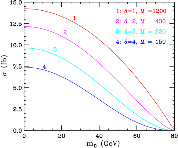
Figure 2: Signal cross-section for $h\chi$ production at LEP with $\sqrt{s}=200$ GeV, for $m_{h}=120$ GeV and different values of $\delta$ and $M$.

For a different $M$, the cross-section can be easily obtained from the scaling relation $\sigma\propto M^{-(\delta+2)}$. The cross-section maxes out at small values of $m_{0}$, when there are more KK states kinematically available. From Fig. 2 we see that if $\delta=n$, the typical maximal values of the cross-section are around 10 fb, in which case only one or two events can be expected at LEP. Of course, the bounds on $M$ from gravity are weaker if one considers cases of $\delta<n$, then LEP might be able to explore the region of very low values of $M$ and small $\delta$. Given the current limits on the Higgs mass, one obviously has to go to a higher energy machine in order to start to see an appreciable signal. We therefore turn to discuss the NLC case in a little bit more detail next.

In Fig. 3 we show a contour plot of the total integrated cross-section at an NLC with $\sqrt{s}=500$ GeV.

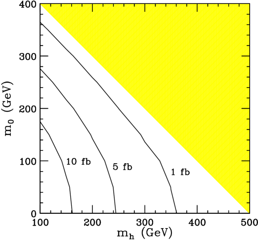
Figure 3: Contour plot of the total cross-section for real flavon emission at the NLC with $\sqrt{s}=500$ GeV, for $y_{f}=1$, $\delta=2$ and $M=1$ TeV. The shaded area is not kinematically accessible at this center-of-mass energy.

We fix $y_{f}=1$, $\delta=2$, $M=1$ TeV and vary the Higgs mass $m_{h}$ and the mass $m_{0}$ of the flavon zero mode. The cross-section shown in Fig. 3 can be easily rescaled for different values of $y_{f}$ or $M$, recall that it scales like $y_{f}^{2}/M^{2+\delta}$. With higher energy and larger integrated luminosity, the flavon production cross-section at the NLC can provide a much more statistically significant signal sample. With 50 ${\rm fb}^{-1}$ of data for the parameters in Fig. 3, one will have a few hundred signal events available. We will then focus our discussion on the question of cuts optimization and increasing the signal-to-background ratio.

The search strategy at the NLC will depend on the Higgs mass. For heavy ($\lower 3.01385pt\hbox{$\;\stackrel{{\scriptstyle\textstyle>}}{{\sim}}\;$}140$ GeV) Higgs masses, the signal will be $WW\not\!\!\!E$, similar to chargino pair production with charginos decaying to real $W$’s and the lightest neutralino. In that case, it is best to reconstruct the $W$’s from the four jet final state [21], where the only non-negligible background is $WWZ$ with $Z\rightarrow\nu\bar{\nu}$, which is on the order of 10 fb [22], after taking into account the $Z$ branching ratio into neutrinos. With cleverly designed cuts [23], it is easy to see an excess over the background for a signal of ${\cal O}$(1 fb), which can then be used to put constraints on $m_{0}$, $m_{h}$, and $M$.

If, however, the Higgs mass is below 140 GeV, the search becomes more challenging, since the backgrounds to the $b\bar{b}\not\!\!\!E$ final state are much larger. The dominant background contributions come from $b\bar{b}\nu_{e}\bar{\nu}_{e}$, $b\bar{b}\nu_{\mu}\bar{\nu}_{\mu}$ and $b\bar{b}\nu_{\tau}\bar{\nu}_{\tau}$ final states. Including the SM diagrams with a Higgs into the background, one has a total of 23, 11 and 11 diagrams, respectively. We show the diagrams for the process $e^{+}e^{-}\rightarrow b\bar{b}\nu_{e}\bar{\nu_{e}}$ in Fig. 4.

0.8 0.7                                                                                                                    Figure 4: The diagrams for the process $e^{+}e^{-}\rightarrow b\bar{b}\nu_{e}\bar{\nu}_{e}$. The subset without $W$ bosons applies for $e^{+}e^{-}\rightarrow b\bar{b}\nu_{\mu}\bar{\nu}_{\mu}$ and $e^{+}e^{-}\rightarrow b\bar{b}\nu_{\tau}\bar{\nu}_{\tau}$.

The diagrams for the processes $e^{+}e^{-}\rightarrow b\bar{b}\nu_{\mu}\bar{\nu}_{\mu}$ and $e^{+}e^{-}\rightarrow b\bar{b}\nu_{\tau}\bar{\nu}_{\tau}$ are obtained by obvious replacements and dropping the diagrams containing a $W$ boson. Notice that most often the two b-jets are not coming from a Higgs, so one can use a ($m_{h}$ dependent) invariant mass cut on the b-jets. The optimal mass window will depend on the features of the particular detector, for our study here we shall take $|m_{bb}-m_{h}|<10$ GeV. In addition, the availability of highly polarized beams at the NLC can substantially suppress the background (which necessarily involves the production of $W$ or $Z$ bosons), since $W$’s only couple to left-handed leptons. Finally, the $ZZ$ background with one $Z$ decaying invisibly can be further suppressed by requiring that the missing mass $M\!\!\!\!/$ in the interaction is not near $M_{Z}$. The remaining $WWZ$ background is small and can be further reduced by a lepton veto.

We used the COMPHEP event generator [24], to simulate the $b\bar{b}\nu\bar{\nu}$ backgrounds (with separate runs for electron and muon/tau neutrinos) and in Fig. 5 show the resulting missing mass $\not\!\!\!M$ distribution at the NLC with $\sqrt{s}=500$ GeV, where we assume a $90\%$ right-polarized electron beam.

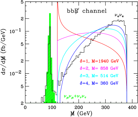
Figure 5: Missing mass distribution of signal and $e^{+}e^{-}\rightarrow b\bar{b}\nu_{i}\bar{\nu}_{i}$ background at the NLC with center-of-mass energy $\sqrt{s}=500$ GeV. The signal distributions are shown for $m_{h}=120$ GeV, $m_{0}=120$ GeV, and several values of $\delta$ and $M$: (a) $\delta=1$, $M=1940$ GeV, (b) $\delta=2$, $M=858$ GeV and (c) $\delta=3$, $M=514$ GeV, (d) $\delta=4$, $M=360$ GeV. All lines are normalized to the correct total cross-section. We have assumed 90% polarization and imposed the cut $|m_{bb}-m_{h}|<10$ GeV. We show the $b\bar{b}\nu_{e}\bar{\nu}_{e}$ background separately from $b\bar{b}\nu_{\mu}\bar{\nu}_{\mu}+b\bar{b}\nu_{\tau}\bar{\nu}_{\tau}$ (shaded).

We also present signal distributions for $m_{h}=120$ GeV, $m_{0}=120$ GeV and several values of $\delta$ and $M$: (a) $\delta=1$, $M=1940$ GeV, (b) $\delta=2$, $M=858$ GeV, (b) $\delta=3$, $M=514$ GeV and (c) $\delta=4$, $M=360$ GeV, where we have picked $M$ so that the total signal cross-section is always 20 fb. We choose to do this since our objective here is to compare the shape of the signal distributions to the shape of the background.

We see from Fig. 5 that the shape of the missing mass distribution for the signal depends on the number of extra dimensions $\delta$. In particular, for $\delta=1$ it exhibits a narrow asymmetric peak near $m_{0}$, for $\delta=2$ it is rather flat, while for larger $\delta$ it starts to peak closer to the largest kinematically allowed values and therefore becomes very similar to the background distribution. (This behavior is easy to understand in terms of the density function – see eq. (A.26) from the Appendix.) Because of the finite detector resolution, the narrow one-sided peak for $\delta=1$ will be smeared and the flavon will look like an ordinary heavy, invisibly decaying neutral particle, so if a signal is seen, an interpretation in terms of the scenario considered here will not be straightforward. Notice that there is very small background with $\not\!\!\!M<M_{Z}$, so by far the easiest case to observe will be $\delta=1$ with $m_{0}<M_{Z}$, since signal and background are very well separated.

3.2 Hadron colliders

In Run II of the Tevatron one can look for a $b\bar{b}{\not\!\!E_{T}}$ final state, which is one of the standard Higgs search channels [25], but without mass reconstruction may also be indicative of several other sources of new physics: bottom squark production [26], stop production with Higgsino LSP [27], leptoquarks [28] etc. We can adapt the existing Run II Higgs analysis of $Zh\rightarrow b\bar{b}{\not\!\!E_{T}}$ for our purposes, keeping in mind that further optimization is possible, e.g. by adjusting the ${\not\!\!E_{T}}$ cut and the $p_{T}$ cuts on the b-jets.

In order to make an estimate of the signal cross-section at the Tevatron, let us first switch the order of integration in (3.20):

$$\sigma_{tot}(E_{\rm CM})\ =\ \int_{m_{0}}^{E_{\rm CM}-m_{h}}dm_{\bf n}\,2m_{\bf n}\rho(m_{\bf n})\int_{x({m_{\bf n}})}^{1}dx_{1}\int_{x({m_{\bf n}})\over x_{1}}^{1}dx_{2}f^{p}(x_{1})f^{\bar{p}}(x_{2})\sigma_{\bf n}({m_{\bf n}},x_{1}x_{2}E^{2}_{CM})$$ (3.21)

where $x({m_{\bf n}})\equiv({m_{\bf n}}+m_{h})^{2}/E^{2}_{CM}$. Then, as long as we are interested in the total signal cross-section only, and not in the resulting kinematic distributions, we can use COMPHEP, for example, to first compute the differential cross-section at a given ${m_{\bf n}}$

$$\sigma_{\bf n}({m_{\bf n}},E_{\rm CM})\ \equiv\ {1\over\rho({m_{\bf n}})}{d\sigma_{tot}\over dm_{\bf n}^{2}}\ =\ \int_{x({m_{\bf n}})}^{1}dx_{1}\int_{{x({m_{\bf n}})\over x_{1}}}^{1}dx_{2}f^{p}(x_{1})f^{\bar{p}}(x_{2})\sigma_{\bf n}({m_{\bf n}},x_{1}x_{2}E^{2}_{CM})$$

and then numerically integrate over ${m_{\bf n}}$.

In Fig. 6 we show a plot of the differential signal cross-section $\sigma_{\bf n}({m_{\bf n}},2\,{\rm TeV})$ before cuts.

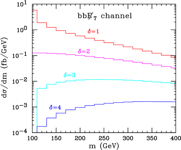
Figure 6: Plot of the signal cross-section for real flavon emission at the Tevatron for $m_{h}=120$ GeV, $m_{0}=100$ GeV, $M=500$ GeV and several values of $\delta$.

Here we include the signal contribution only from real flavon emission and not from $Zh$. Notice that depending on the flavor of the quarks participating in the hard scattering, different species of flavons will be produced. However, we assume that they all escape the detector and give rise to ${\not\!\!E_{T}}$. For the plot we have made the simplifying assumption that the couplings $y_{f}$ are universal and that the mass of the zero mode $m_{0}$ is the same for all species of flavons.

In Fig. 6 we observe the typical dependence of the mass distribution on the number of extra dimensions $\delta$, already familiar from Fig. 5. We see that for $\delta>2$ the distributions peak at rather large values of ${m_{\bf n}}$ of around 300-400 GeV. Notice, however, that although the actual missing energy in those events will be very large (typically on the order of a few hundred GeV), the distribution of the measured ${\not\!\!E_{T}}$ will be much softer. The measured ${\not\!\!E_{T}}$ in the detector is determined by the energy of the visible products, in our case the two b-jets, which is not much above $m_{h}/2$. Nevertheless, we remind the reader that the Higgs search in Run IIb will be sensitive to raw $b\bar{b}{\not\!\!E_{T}}$ cross-sections on the order of 26 fb [25]. We then see from Fig. 6 that flavon searches in the same channel may yield very strong bounds on $M$, for example, we can see from the plot that $M\lower 3.01385pt\hbox{$\;\stackrel{{\scriptstyle\textstyle<}}{{\sim}}\;$}1000,\,500,\,300,\,200$ GeV for $\delta=1,\,2,\,3,\,4$ respectively can be easily ruled out.

At a $pp$ collision machine like LHC, the initial state anti-fermion must come from a sea quark, which will suppress the production cross-section. At the LHC it will be very hard to observe the $b\bar{b}{\not\!\!E_{T}}$ final state, instead one typically has to utilize the decays $h\rightarrow\gamma\gamma$ and/or $h\rightarrow ZZ$. The possibility of producing an additional invisible flavon state in the interaction gives rise to unique clean signatures like $\gamma\gamma{\not\!\!E_{T}}$ (for low Higgs masses) or $\ell\ell\ell\ell{\not\!\!E_{T}}$ (for higher Higgs masses).

4 Virtual Flavon exchange

Throughout this section we shall assume that each flavon only couples to the corresponding pair of fermions. Then, virtual flavon exchange at an $e^{+}e^{-}$ machine can only give back final states with electrons and positrons, while flavon exchange at a hadron collider will yield signatures with jets.

Virtual flavons can mediate processes with 2-fermion, 4-fermion or 6-fermion final states. The corresponding Feynman diagrams for an $e^{+}e^{-}$ lepton collider are shown in Figs. 7, 8 and 9, respectively (for a hadron collider, just replace $e\rightarrow q$).

1.2 1.0           Figure 7: The diagrams for the process $e^{+}e^{-}\rightarrow\chi^{\ast}\rightarrow e^{+}e^{-}$.

1.2 1.0        

Figure 8: The diagrams for the process $e^{+}e^{-}\rightarrow\chi^{\ast}\rightarrow e^{+}e^{-}b\bar{b}$.

1.2 1.0                               Figure 9: The diagrams for the process $e^{+}e^{-}\rightarrow\chi^{\ast}h\rightarrow e^{+}e^{-}hh$. Each Higgs further decays to a $b\bar{b}$ or $\tau^{+}\tau^{-}$ pair.

For $\delta>2$, the virtual $\chi$ exchange can be represented by a local effective dimension 8 operator (A.31) as shown in the Appendix. In Table 3 we list the signal cross-sections (in fb) from this effective operator at different colliders for $\Lambda_{T}=1$ TeV and $m_{h}=120$ GeV.

Final	LEP	NLC	FNAL	LHC
state	200 GeV	500 GeV	2 TeV	14 TeV
$ff$	0.95	$5.91$	12.9	373
$ffh$	$9\times 10^{-5}$	$6\times 10^{-2}$	$2.8\times 10^{-2}$	60
$ffhh$	—	$6.5\times 10^{-6}$	$2.9\times 10^{-4}$	2.7

Table 3: Signal cross-sections in fb for the 2-fermion, 4-fermion ($f\bar{f}b\bar{b}$) and 6-fermion ($f\bar{f}b\bar{b}b\bar{b}$) final states, at various colliders (with their center of mass energy shown) and for $\Lambda_{T}=1$ TeV and $m_{h}=120$ GeV.

In the case of a real Higgs production, we only consider decays to $b\bar{b}$ final states, whose branching fraction was computed with the HDECAY program [29]. If $\Lambda_{c}=M$ and $y_{f}=1$, then $\Lambda_{T}=1$ TeV corresponds to $M=400,237,145$ GeV for $\delta=3,\,4,\,5$, respectively. These cross-sections can be readily rescaled for different values of $\Lambda_{T}$, recall that $\sigma\sim\Lambda_{T}^{-8}$.

We see from Table 3 that the signal cross-sections are rather small, and just like in the case of virtual graviton exchanges, one will have to look for interference effects instead, since those are only proportional to $\Lambda_{T}^{-4}$.

For $\delta\leq 2$, the effective interaction still depends on the momentum flow along the $\chi$ propagator. In the case of $\delta=2$, there is only a mild logarithmic dependence on the momentum and the cutoff. The case of $\delta=1$ is more interesting. The integral over KK states is convergent, therefore independent of the cutoff. For $p^{2}>m_{0}^{2}$ ($p$ is the momentum of the $\chi$ field), the effective interaction is imaginary, corresponding to real $\chi$ production. Whether it gives rise to the same final state particles or not, depends on the $\chi$ lifetime. Real $\chi$ production does not interfere with other virtual (off-shell) processes. The singularity at $p^{2}=m_{0}^{2}$ will be smoothed out by the decay width of the $\chi$ fields and the detector resolution. Nevertheless, the peak at $p^{2}=m_{0}^{2}$ provides an extra handle of the $\delta=1$ case.

In the rest of this Section we shall discuss lepton and hadron colliders separately.

4.1 Lepton colliders

The virtual scalar exchanges in Fig. 7 will modify the angular distribution of the leptons in Bhabha scattering and may be detected at LEP. In Fig. 10 we show the differential cross-section $d\sigma/d\cos\theta$ (in fb) at LEP for $\Lambda_{T}=750$ GeV, where $\theta$ is the scattering angle of the electron with respect to the direction of the electron beam.

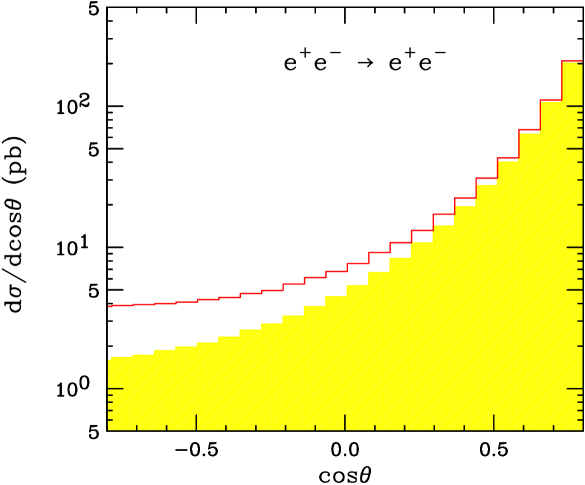
Figure 10: Angular distribution for both signal and background at LEP with $\sqrt{s}=200$ GeV in Bhabha scattering, for $\Lambda_{T}=750$ GeV.

The shaded histogram is just the background contribution, while the solid histogram includes both signal and background. There is a visible excess of backscattered electrons, which is typical of the (isotropic) scalar exchange. In order to extract the LEP limits on $\Lambda_{T}$ from Bhabha scattering, we can apply the latest bounds on the relevant compositeness scale $\Lambda_{\rm LR}$ [30]. We have to equate the coefficient of the contact term

$${g^{2}\over 2\Lambda^{2}_{\rm LR}}(\bar{e}_{L}\gamma^{\mu}e_{L})(\bar{e}_{R}\gamma_{\mu}e_{R})\sim{g^{2}\over\Lambda^{2}_{\rm LR}}(\bar{e}_{L}e_{R})(\bar{e}_{R}e_{L})$$ (4.22)

to the coefficient of the effective operator (A.31). The typical bounds on $\Lambda_{\rm LR}$ of 4.5 TeV for $g^{2}\sim 4\pi$ then translate into

$$\Lambda_{T}\lower 3.01385pt\hbox{$\;\stackrel{{\scriptstyle\textstyle>}}{{\sim}}\;$}\left({v\Lambda_{\rm LR}\over\sqrt{4\pi}}\right)^{1/2}\sim 525\ {\rm GeV}.$$ (4.23)

We should point out that in the case of $\delta=1$ and $m_{0}$ not near $M_{Z}$, one may use in addition the peak in the invariant mass of the leptons.

We next discuss the 4-fermion channel, which is similar to the existing $Zh\rightarrow e^{+}e^{-}b\bar{b}$ searches [15]. Here the invariant mass $m_{e^{+}e^{-}}$ of the $e^{+}e^{-}$ pair is not constrained to be close to $M_{Z}$, so one might think that $m_{e^{+}e^{-}}$ will be a useful variable to cut on. In Fig. 11 we show the $m_{e^{+}e^{-}}$ distribution in $e^{+}e^{-}h^{0}$ events for signal plus background (solid) or just the background (shaded) at an NLC with $\sqrt{s}=500$ GeV, and for $\Lambda_{T}=600$ GeV and $m_{h}=120$ GeV.

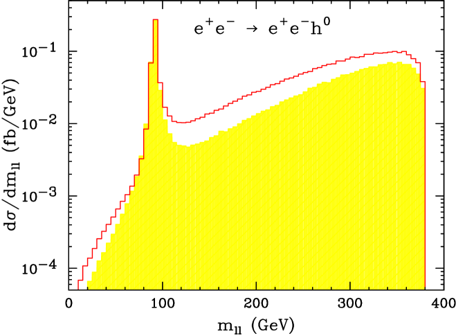
Figure 11: Invariant mass distribution of the $e^{+}e^{-}$ pair in $e^{+}e^{-}h^{0}$ events for both signal (solid) and background (shaded) at the NLC with $\sqrt{s}=500$ GeV, and for $\Lambda_{T}=600$ GeV and $m_{h}=120$ GeV.

We see that $m_{e^{+}e^{-}}$ does not allow good discrimination between signal and background, since the two distributions are very similar. Above the $Z$-peak, the background is dominated by $Z$-fusion, just like $W$-fusion was the main background for the $b\bar{b}{\not\!\!E_{T}}$ channel in Section 3.1. Unlike $W$-fusion, here we have the additional advantage that we can measure the angular distribution of the individual leptons. This might be useful because the leptons in $Z$-fusion tend to be forward, while the leptons from the signal are isotropic. This is illustrated in Fig. 12, where

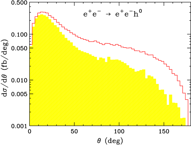
Figure 12: The same as Fig 11, but for the angular distribution $d\sigma/d\theta$, where $\theta$ is the scattering angle of the electron with respect to the electron beam.

we show the angular distribution of the electron with respect to the electron beam for the same parameters as in Fig. 11. We see that $\theta$ can be a decent discriminator between signal and background.

And finally, given the current limits on $m_{h}$, the 6-fermion final state is not observable at LEP. From Table 3 we estimate that we can record 5 signal events at the NLC with $\sqrt{s}=500$ GeV and total integrated luminosity 50 ${\rm fb}^{-1}$, only if $\Lambda_{T}<300$ GeV. Such low values of $\Lambda_{T}$ are already ruled out by LEP (see eq. (4.23) above).

4.2 Hadron colliders

At hadron colliders we can similarly have 2-jet, 4-jet and 6-jet final states, by replacing $e\rightarrow q$ in Figs. 7, 8 and 9.

The dijet signal should be studied analogously to the graviton exchange [31], the difference now being that the angular distributions should be characteristic of spin 0 rather than spin 2 virtual exchange.

The observation of the 4-jet final state will be rather difficult. There will be large irreducible backgrounds from $t\bar{t}$, $Z+2j$, $WZ$ and $ZZ$, besides, the signal looks just like $gg\rightarrow h$ with extra radiated jets. In any case, the presence of extra jets is not very useful at a hadron machine. Even for larger Higgs masses, where the Higgs decays to gauge bosons, our signal is not distinctive enough by itself and will be simply added to the samples for the regular Higgs search.

The 6-jet final state is cleaner, but the cross-section is too small to be relevant for the Tevatron. However, Higgs pair-production processes have small Standard Model backgrounds. Therefore identification of both Higgs particles in the event can be an important test for the presence of some new physics (see, e.g. [32]). The main Higgs pair-production process at the LHC is gluon fusion [33]. In the four b-jet channel, very high $p_{T}$ cuts on the jets are necessary in order to suppress the QCD backgrounds, and then the acceptance is only 1-2%, assuming rather optimistic b-tagging efficiencies [34]. Therefore, for low Higgs masses it seems rather difficult to see a signal, and almost impossible to distinguish it from $hb\bar{b}$ at large $\tan\beta$. For heavy Higgs masses, where the cross-section is smaller than the one shown in Table 3, we have 4 gauge bosons $+$ 2 jet signatures. Then, for the purposes of both triggering and reducing the background, one would have to use the leptonic decays of a sufficient number of $W$’s and $Z$’s, thus paying a significant price in branching ratios.

5 Conclusions

The possibility that new large compact dimensions may be probed in the near-term future at collider experiments is very exciting. Finding KK excitations will provide a strong evidence for the existence of extra dimensions. On general grounds, one expects that in addition to gravitons, there are other particles feeling the extra dimensions. If they are some SM fields, then looking for their KK excitations will provide the strongest probe of the extra dimensions. The experimental constraints on the masses of the KK modes of the SM fields require the corresponding extra dimensions to have sizes smaller than $\sim{\rm TeV}^{-1}$. If we assume that all SM gauge fields are localized on our brane, any bulk field must be neutral under the SM gauge group. Hence bulk fields will only couple to some neutral combination of the SM fields. In the case of a bulk fermion, it may couple to $\bar{\ell}_{L}\tilde{H}$ and be identified as right-handed neutrino. The smallness of the neutrino masses can then be explained by the large size of the extra dimensions [35, 36]. It may also give rise to invisible Higgs decays [16]. If the bulk field is a scalar, it can couple to neutral combinations of the SM fields such as $\bar{f}_{L}f_{R}H$, $F^{\mu\nu}F_{\mu\nu}$, or higher dimensional ones $QQQL$ and so on. The study of this paper can apply to any scalar bulk fields which couple to $\bar{f}_{L}f_{R}H$, independent of whether there is a flavor theory. The scalars which couple to $F^{\mu\nu}F_{\mu\nu}$ are similar to the dilatons and will be left for future studies. The scalars which couple to higher dimensional SM operators like $QQQL$, have suppressed interactions and are therefore much more difficult to produce in collider experiments.

The new signals studied in this paper are not limited to the ideas of large extra dimensions. Ignoring for the moment the difficulties in flavor model building, the results are also applicable in the usual four dimensional flavor theories if the flavons are light. In spite of the differences in the invariant mass distribution of the flavon (or its decay products), it seems that distinguishing between a four dimensional and a higher dimensional flavon scenario is intrinsically quite difficult and may have to wait for even more advanced experimental facilities.

To summarize, we have studied many new signals coming from flavor physics within the framework of large extra dimensions and TeV scale gravity. These new signatures are particularly interesting because they are associated with the Higgs boson, which is the only missing piece of the Standard Model and hence the most hunted particle. We find that the production of Higgs + real flavon could probe the string scale just as well as the KK graviton production at the current and future colliders, if the flavons and the graviton live in the same number of extra dimesions. However, if the flavons only live in a subspace of the extra dimensions accesible to the graviton, associated flavon-Higgs production can provide stronger constraints than graviton production. In addition, there is a range of the parameter space in which the flavons can have macroscopic decay lengths, which will give rise to the spectacular signals of displaced vertices. The virtual flavon exchange generates higher dimensional operators which contain Higgs fields. However, they do not provide as good probes as the real flavon emission, because the backgrounds are very large for final states with 0 or 1 Higgs bosons, while the clean signals of 2 Higgs final states are too small to be observed. A possible exception is the case in which the flavons only live in one extra dimension. The fermion pair invariant mass peaks at the mass of the flavon zero mode, providing a very distinctive signal. This is a novel feature of the flavons in one extra dimension, since one extra dimension for the graviton in the TeV scale gravity scenario is ruled out. Note that in our study we have made the conservative assumption that each flavon only couples to one corresponding fermion pair. There could be more promising signals if one relaxes this assumption. For instance, if a flavon couples to both quarks and leptons, then at a hadron collider we can have $b\bar{b}$ (from $h$) + leptons final states, which is an exceptionally clean signal.

Acknowledgements: We would like to thank N. Arkani-Hamed, J. Bagger, S. Dimopoulos, L. Hall, G. Landsberg and J. Lykken for stimulating discussions. Fermilab is operated by the URA under DOE contract DE-AC02-76CH03000.

Appendix A Formalism and conventions

Expanding $H$ and $\chi$ around their vevs, $H=(0,\,(v+h)/\sqrt{2})$ (setting the would-be-Goldstone fields to zero) and $\chi_{\bf n}=\left\langle\chi_{\bf n}\right\rangle+\chi^{\prime}_{\bf n}$, the interactions (1.7) contain

$${\cal H}_{\rm int}\supset m_{f}{\bar{f}}_{L}f_{R}+{\lambda_{f}\over\sqrt{2}}{\bar{f}}_{L}f_{R}h+\sum_{\bf n}{y_{f}v\over\sqrt{2}M_{F}}{\bar{f}}_{L}f_{R}\chi^{\prime}_{\bf n}+\sum_{\bf n}{y_{f}\over\sqrt{2}M_{F}}{\bar{f}}_{L}f_{R}h\chi^{\prime}_{\bf n}+{\rm h.c.},$$ (A.24)

where $v=246$ GeV is the Higgs vev, $m_{f}$ and $\lambda_{f}$ are the mass and Yukawa coupling for the corresponding fermion, $h$ is the real Higgs field and $\chi^{\prime}_{\bf n}$ are complex KK states. For simplicity, we assume that the masses of the real and the imaginary parts of $\chi^{\prime}$ are the same. The mass for the KK state $\chi_{\bf n}$ is given by $m_{\bf n}^{2}=m_{0}^{2}+4\pi^{2}|{\bf n}|^{2}/L^{2}$, where $m_{0}$ is the mass of the zero mode. Also, for notational simplicity, we will omit the prime on $\chi^{\prime}$ for the most part of the paper: $\chi$ is understood as the vev shifted field when there is no confusion.

We follow the approach of Han, Lykken, and Zhang [37], changing slightly their notation: $R\rightarrow L$ for the length of the extra dimensions and $n\rightarrow\delta$ for the number of extra dimensions accessible to $\chi$’s. Because there is a mass $m_{0}$ for the zero mode, the number of KK states of $\chi$ in the mass interval $dm_{\bf n}^{2}$ is now given by

$$dN\approx\rho(m_{\bf n})dm_{\bf n}^{2},$$ (A.25)

with

$$\rho(m_{\bf{}_{n}})={L^{\delta}(m_{\bf n}^{2}-m_{0}^{2})^{(\delta-2)/2}\over(4\pi)^{\delta/2}\Gamma(\delta/2)}.$$ (A.26)

The effective interaction due to the virtual $\chi$ KK state exchange can be obtained by summing over the KK state propagator, in a way similar to the virtual KK graviton exchange [6, 37, 38]. For $\delta\geq 2$ the virtual exchange is dominated by the high KK states, it depends sensitively on the cutoff scale $\Lambda_{c}$, but not on $m_{0}$, as long as $m_{0}$ is much smaller than $\Lambda_{c}$ (and $\sqrt{s},\,\sqrt{|t|}$ for $\delta=2$). The sum over the KK mode propagators gives

$$D(s) = \int_{m_{0}^{2}}^{\Lambda_{c}^{2}}\ dm^{2}_{\bf n}\ \rho(m_{\bf n})\ {i\over s-m^{2}_{\bf n}+i\varepsilon}$$ (A.27)

$$\approx \left\{\begin{array}[]{l}{L^{2}\over 4\pi}\ \biggl{[}\pi-i\ln\biggl{(}{\Lambda^{2}_{c}-s\over s-m_{0}^{2}}\biggr{)}\biggr{]},\quad\delta=2;\\[5.69054pt] {2L^{\delta}(s-m_{0}^{2})^{(\delta-2)/2}\over(\delta-2)\Gamma(\delta/2)(4\pi)^{\delta/2}}\Biggl{[}\pi-i\biggl{(}{\Lambda_{c}^{2}-m_{0}^{2}\over s-m_{0}^{2}}\biggr{)}^{(\delta-2)/2}\Biggr{]},\quad\delta>2.\end{array}\right.$$ (A.30)

The real part represents the real KK mode production. It contributes to the same processes as the virtual exchange only if the KK mode of $\chi$ has prompt decay. It is smaller than the virtual contribution if $\Lambda_{c}\gg\sqrt{s},\,m_{0}$ for $\delta\geq 2$. The $t$-channel exchange can be obtained similarly by replacing $s$ by $t$ (remembering that $t<0$).

The virtual exchange for $\delta>2$ is independent of $s$ and therefore can be written as an effective dimension 8 operator, assuming $\Lambda_{c}\gg m_{0}$ and using $M_{F}^{2}=M^{2+\delta}L^{\delta}$,

$${\cal H}_{\rm eff} = -{|y_{f}|^{2}\over(\delta-2)\Gamma(\delta/2)(4\pi)^{\delta/2}}{\Lambda_{c}^{\delta-2}\over M^{2+\delta}}|\bar{f}_{L}f_{R}h|^{2}$$ (A.31)

$$\equiv -{1\over\Lambda_{T}^{4}}|\bar{f}_{L}f_{R}h|^{2},$$

Experiments on virtual exchange only probe the coefficient of this effective operator, $\Lambda_{T}^{4}$, which is a combination of the gravitation scale $M$ and the cutoff $\Lambda_{c}$. Because the cutoff is not known, the experimental probes of virtual exchange processes should not be directly compared to the real $\chi$ production.

For $\delta=2$, the virtual $\chi$ exchange still depends logarithmically on the momentum flow through $\chi$. In analogy to (A.31), we will write the effective interaction as

$$-{|y_{f}|^{2}\over 8\pi M^{4}}\ln\biggl{|}{\Lambda_{c}^{2}-p^{2}\over p^{2}-m_{0}^{2}}\biggr{|}|\bar{f}_{L}f_{R}h|^{2},$$ (A.32)

where $p^{2}$ is the momentum flow of the virtual $\chi$.

For $\delta=1$, the integral over KK propagators is convergent,

$$D(s)={L\over 2}{1\over\sqrt{s-m_{0}^{2}}}+i{L\over\pi}{1\over\sqrt{\Lambda_{c}^{2}-m_{0}^{2}}}.$$ (A.33)

If $\Lambda_{c}$ is taken to be infinity, the second term can be dropped. For $s>m_{0}^{2}$, it is dominated by real $\chi$ production. The final state depends on whether $\chi$ decay inside or ouside the detector. For $s<m_{0}^{2}$ or $t$-channel exchange, the effective interaction is

$$-{|y_{f}|^{2}\over 4M^{3}}{1\over\sqrt{m_{0}^{2}-p^{2}}}|\bar{f}_{L}f_{R}h|^{2}.$$ (A.34)

The singularity at $p^{2}=m_{0}^{2}$ will be smoothed out by the decay width of the $\chi$ KK states.

There are also interactions with one or both $h$ replaced by their vev. For $\delta>2$, the effective operators (A.31) are independent of the momentum. They can be implemented in COMPHEP via the exchange of an auxiliary field, without the need to consider $t$-channel and $u$-channel contributions separately. They are automatically accounted for by COMPHEP in the process of constructing all Feynman diagrams for the particular process.

References

- [1] C. D. Froggatt and H. B. Nielsen, Nucl. Phys. B147, 277 (1979).
- [2] R.N. Cahn and H. Harari, Nucl. Phys. B176 (1980) 135.
- [3] N. Arkani-Hamed, C.D. Carone, L.J. Hall and H. Murayama, Phys. Rev. D54 (1996) 7032 hep-ph/9607298.
- [4] N. Arkani-Hamed, S. Dimopoulos and G. Dvali, Phys. Lett. B429, 263 (1998), hep-ph/9803315; Phys. Rev. D59, 086004 (1999), hep-ph/9807344.
- [5] N. Arkani-Hamed and S. Dimopoulos, preprint SLAC-PUB-8008, hep-ph/9811353.
- [6] G. F. Giudice, R. Rattazzi and J. D. Wells, Nucl. Phys. B544, 3 (1999), hep-ph/9811291.
- [7] E.A. Mirabelli, M. Perelstein, and M.E. Peskin, Phys. Rev. Lett. 82, 2236 (1999)hep-ph/9811337.
- [8] S. Cullen and M. Perelstein, Phys. Rev. Lett. 83, 268 (1999), hep-ph/9903422.
- [9] L.J. Hall and D. Smith, preprint LBNL-43091, hep-ph/9904267.
- [10] N. Arkani-Hamed, S. Dimopoulos, L.J. Hall, D. Smith, and N. Weiner, talk presented by L.J. Hall at SUSY99, Fermilab, June 21-26, 1999.
- [11] B. S. Chivukula and H. Georgi, Phys. Lett. B188, 99 (1987).
- [12] K. Cheung and W.-Y. Keung, preprint UCD-HEP-99-6, hep-ph/9903294.
- [13] C. Balazs, H.-G. He, W. Repko, C.-P. Yuan and D. Dicus, preprint MSU-HEP-90105, hep-ph/9904220.
- [14] For an updated review of the various Higgs searches at the Tevatron, see http://fnth37.fnal.gov/higgs.html.
- [15] LEP Working Group for Higgs boson searches, ALEPH 99-081, DELPHI 99-142, L3 Note 2442; OPAL Technical Note TN 614.
- [16] S. Martin and J. Wells, preprint FERMILAB-PUB-99-037-T, hep-ph/9903259.
-
[17]
M. Acciarri et al.,
Phys. Lett. B418, 389 (1998);
R. Barate et al., Phys. Lett. B450, 301 (1999). -
[18]
J. Conway, Nucl. Phys. Proc. Suppl. 55C, 409, 1997;
M. Gallinaro, Nucl. Phys. Proc. Suppl. 65, 147, 1998. - [19] D. Cutts and G. Landsberg, hep-ph/9904396, contributed to Physics at Run II: QCD and Weak Boson Physics Workshop, Batavia, IL, 4-6 Mar 1999.
- [20] H.-C. Cheng, B.A. Dobrescu and K.T. Matchev, Phys. Lett. B439, 301 (1998), hep-ph/9807246; Nucl. Phys. B543, 47 (1999), hep-ph/9811316.
- [21] JLC-I, by the JLC Group, preprint KEK 92-16, 1992.
- [22] H. Murayama, Ph. D. Thesis, preprint UT-580, 1991.
-
[23]
J.-F. Grivaz, in “ collisions at 500 GeV: The
Physics Potential”, ed. by P. M. Zervas,
DESY Report 92-123A/B, Hamburg, 1992;
T. Tsukamoto, K. Fujii, H. Murayama, M. Yamaguchi and Y. Okada, Phys. Rev. D51, 3153 (1995). -
[24]
P. A. Baikov et al., “Physical results by means of CompHEP”,
in Proc. of the X Workshop on High Energy Physics and
Quantum Field Theory (QFTHEP-95),
ed. by B. Levtchenko and V. Savrin, Moscow, 1996, p. 101,
hep-ph/9701412;
E. Boos, M. Dubinin, V. Ilyin, A. Pukhov and V. Savrin, hep-ph/9503280. -
[25]
D. Hedin and V. Sirotenko, D0 note 3919, also available on the web:
http://fnth37.fnal.gov/higgs/hedin.html;
W. Yao, talk given at the Higgs Working Group parallel session November 21, 1998, as part of the Supersymmetry–Higgs Summary Meeting, http://fnth37.fnal.gov/higgs/weiming.html. - [26] B. Abbott et al., Phys. Rev. D60, 031101 (1999), hep-ex/9903041.
- [27] K. Matchev, talk given at SUSY’98, Oxford, England, a copy of the transparencies available at http://hepnts1.rl.ac.uk/SUSY98.
- [28] B. Abbott et al., Phys. Rev. Lett. 81, 38 (1998), hep-ex/9803009.
- [29] A. Djouadi, J. Kalinowski and M. Spira, Comp. Phys. Comm. 108, 56 (1998), hep-ph/9704448.
-
[30]
L3 Collaboration (M. Acciarri et al.),
Phys. Lett. B439, 183 (1998);
ALEPH Collaboration (R. Barate et al.), CERN-EP-99-042, hep-ex/9904011 ;
OPAL Collaboration (G. Abbiendi et al.), CERN-EP-99-097, hep-ex/9908008. - [31] P. Mathews, S. Raychaudhuri and K. Sridhar, preprint TIFR-TH-99-13, hep-ph/9904232.
- [32] T. Rizzo, preprint SLAC-PUB-8071, hep-ph/9903475.
-
[33]
S. Dawson, S. Dittmaier and M. Spira,
Phys. Rev. D58, 115012 (1998), hep-ph/9805244;
A. Djouadi, W. Kilian, M. Muhlleitner and P.M. Zerwas, Eur. Phys. J. C10, 45 (1999), hep-ph/9904287. - [34] E. Richter-Was and D. Froidevaux, Zeit. Phys. C76, 665 (1997), hep-ph/9708455.
- [35] N. Arkani-Hamed, S. Dimopoulos, G. Dvali and J. March-Russell, preprint SLAC-PUB-8014, hep-ph/9811448.
- [36] K.R. Dienes, E. Dudas and T. Gherghetta, preprint CERN-TH-98-370, hep-ph/9811428.
- [37] T. Han, J. D. Lykken and R.-J. Zhang, Phys. Rev. D59, 105006 (1999), hep-ph/9811350.
- [38] J. L. Hewett, SLAC-PUB-8001, hep-ph/9811356.