Precision Observables and Electroweak Theories

Abstract

We compute the bounds from precision observables on alternative theories of electroweak symmetry breaking. We show that a cut-off as large as 3 TeV can be accomodated by the present data, without unnatural fine tuning.

]

I Introduction

During the past few years, precision measurements of electroweak observables have probed the standard model of particle physics to the 0.1% level. They now give a 95% C.L. upper bound of 230 GeV on the mass of the standard model Higgs boson [1]. Precision measurements have also constrained many alternative theories to the standard model. For example, they have ruled out many of the most naive technicolor theories [2].

The theory of effective Lagrangians provides a convenient way to describe the low-energy effects of new physics beyond the standard model. One approach is to take the standard model with a fundamental Higgs boson and add a set of $SU(3)\times SU(2)\times U(1)$ invariant higher-dimensional operators, suppressed by a scale $\Lambda$. These operators are assumed to be generated by new physics at the scale $\Lambda$, beyond that of the usual standard model. Because the effective theory includes a fundamental Higgs boson, triviality gives the only upper bound on the scale $\Lambda$. This approach has recently been used to study the Higgs mass limit that comes from precision measurements. It was shown that the new operators can raise the limit on the Higgs mass as high as 400-500 GeV, barring unnatural cancellations [3].

A second approach is to eliminate the Higgs entirely and parametrize the present data in terms of the standard model fields that have been discovered to date. In this approach, $\Lambda$ defines the scale of the physics responsible for electroweak symmetry breaking. At low energies, all effects of this physics can be described by a gauge invariant chiral Lagrangian, in which the higher-dimensional operators are suppressed by $\Lambda$. This approach is valid for energies $E\raise 1.29167pt\hbox{$\,<$\kern-7.5pt\lower 4.30554pt\hbox{$\sim$}\,}\Lambda$. General unitarity considerations restrict $\Lambda\raise 1.29167pt\hbox{$\,<$\kern-7.5pt\lower 4.30554pt\hbox{$\sim$}\,}3$ TeV.

In this letter we pursue this second approach and focus on the physics of electroweak symmetry breaking. We will use the precision measurements to constrain the coefficients of the leading higher dimensional operators in the chiral Lagrangian, as a function of the scale $\Lambda$. We will find that even for $\Lambda\approx 3\,$TeV, the present precision data can be accomodated without unnatural fine tuning.

If $\Lambda\simeq 3$ TeV, the physics of electroweak symmetry breaking lies outside the reach of the LEP and Tevatron colliders. Our analysis indicates that this possibility remains open, despite the 230 GeV lower limit on the mass of the standard model Higgs. We shall see that the data is perfectly consistent with theories in which there are no new particles below 3 TeV. Of course, it is an open question whether such theories can actually be constructed, consistent with the data. Nevertheless, our results point to a loophole in the common assertion that the precision data require a Higgs boson or other new physics to be close at hand.

The plan of this letter is as follows. We start by presenting the gauged chiral Lagrangian associated with electroweak symmetry breaking. We then focus on the two operators that are most important for precision measurements on the $Z$ pole. We compute the effects of these operators on experimental observables and derive limits on their coefficients as a function of the scale $\Lambda$. Finally, we discuss our results in the context of alternative scenarios for electroweak symmetry breaking.

II Framework

The gauged chiral Lagrangian provides a model-independent description of the physics that underlies electroweak symmetry breaking.[4, 5] It is valid for energies $E\raise 1.29167pt\hbox{$\,<$\kern-7.5pt\lower 4.30554pt\hbox{$\sim$}\,}\Lambda$, where the new physics becomes manifest.

The Lagrangian is constructed from the Goldstone bosons $w^{a}$ associated with breaking $SU(2)\times U(1)\rightarrow U(1)$. The fields $w^{a}$ are assembled into the group element $\Sigma=\exp(2iw^{a}\tau^{a}/v)$, where the $\tau^{a}$ are Pauli matrices, normalized to $1/2$, and $v=256$ GeV is the scale of the symmetry breaking. The fields $w^{a}$ transform nonlinearly under $SU(2)\times U(1)$ transformations, $\Sigma\to L\Sigma R^{\dagger}$, where $L\in SU(2)\equiv SU(2)_{L}$ and $R\in U(1)\subset SU(2)_{R}$. The gauge bosons appear through their field strengths, $W_{\mu\nu}=W^{a}_{\mu\nu}\tau^{a}$ and $B_{\mu\nu}=B^{3}_{\mu\nu}\tau^{3}$, as well as through the covariant derivative, $D_{\mu}\Sigma=\partial_{\mu}\Sigma+igW^{a}_{\mu}\tau^{a}\Sigma-ig^{\prime}\Sigma B^{3}_{\mu}\tau^{3}$.

The gauged chiral Lagrangian is built from these objects. It can be organized in a derivative expansion,

$${\cal L}={\cal L}^{(2)}+{\cal L}^{(4)}+\ldots,$$ (1)

where

$${\cal L}^{(2)} = \ \ {v^{2}\over 4}\,{\rm Tr\,}D_{\mu}\Sigma D_{\mu}\Sigma^{\dagger}+{{g^{\prime}}^{2}v^{2}\over 16\pi^{2}}\,b_{1}\,({\rm Tr\,}T\,\Sigma^{\dagger}D_{\mu}\Sigma)^{2}$$ (3)

$$\mbox{}+{gg^{\prime}\over 16\pi^{2}}\,a_{1}\,{\rm Tr\,}B_{\mu\nu}\Sigma^{\dagger}W_{\mu\nu}\Sigma\,,$$

and $T=\Sigma^{\dagger}\tau^{3}\Sigma$. The Lagrangian is invariant under $SU(2)\times U(1)$ gauge transformations. In the unitary gauge, with $\Sigma=1$, the terms in ${\cal L}^{(2)}$ give rise to the $W$ and $Z$ masses. The terms in ${\cal L}^{(4)}$ give rise to “anomalous” three- and four-gauge boson self couplings.

The coefficients $a_{1}$ and $b_{1}$ are important because they contain information about the physics of electroweak symmetry breaking. Note that the operator proportional to $a_{1}$ preserves weak isospin in the limit $B^{3}_{\mu}\rightarrow 0$, while the one proportional to $b_{1}$ does not. The coefficients are obtained by matching Green functions in the effective theory with those of the underlying fundamental theory, just below the scale $\Lambda$. The coefficients $a_{1}$ and $b_{1}$ are normalized so that they are naturally ${\cal O}(1)$ for a strongly interacting sector with $\Lambda\simeq 3$ TeV. They can be much smaller if the symmetry-breaking sector is weakly coupled; they can be larger if the fundamental theory contains many particles charged under $SU(2)\times U(1)$.

In what follows we will study the effects of $a_{1}$ and $b_{1}$ on the $W$ and $Z$ propagators. These coefficients are closely related to the parameters $S$ and $T$. The relation is found by renormalizing the coefficients from $\Lambda$ to the scale $M_{Z}$, where $S$ and $T$ are defined. One finds

$$S = S_{0}+{1\over 6\pi}\,\log\left(\Lambda\over M_{Z}\right),$$ (4)

$$T = T_{0}-{3\over 8\pi c^{2}}\,\log\left(\Lambda\over M_{Z}\right),$$ (5)

where $c=\cos\theta_{W}$, and $S_{0}$ and $T_{0}$ are fixed in terms of $a_{1}$ and $b_{1}$ at the scale $\Lambda$,

$$S_{0}=-{a_{1}\over\pi}\,,\qquad\qquad T_{0}={b_{1}\over\pi c^{2}}\,.$$ (6)

Note that the logarithms are exactly calculable because they come from standard model loops. (We assume explicitly that there are no light particles, such as pseudo-Goldstone bosons, with masses between $\Lambda$ and $M_{Z}$ [6].) Equation (5) connects the new physics at the scale $\Lambda$ with precision measurements at the scale $M_{Z}$.

III Results

We are now ready to find the constraints imposed by precision electroweak measurements on $S$ and $T$, and consequently, on the scale $\Lambda$ and the coefficients $a_{1}$ and $b_{1}$.

Most global analyses of precision electroweak data are carried out in the context of the standard model with a fundamental Higgs boson. Fortunately, these analyses can be easily converted to the case at hand. One simply subtracts the contributions to $S$ and $T$ from a standard model Higgs boson, and then adds back the contribution from equation (5). In this way one can readily compute the values of $S$ and $T$ that come from the gauged chiral Lagrangian.

The contributions to $S$ and $T$ from a heavy Higgs have been computed in the literature.[5] They are

$$S = -{1\over 6\pi}\,\Bigg{[}{5\over 12}-\log\left({M_{H}\over M_{Z}}\right)\Bigg{]},$$ (7)

$$T = {3\over 8\pi c^{2}}\,\Bigg{[}{5\over 12}-\log\left({M_{H}\over M_{Z}}\right)\Bigg{]},$$ (8)

where the constant is computed in the $\overline{{\rm MS}}$ scheme. Note that the logarithmic dependence on the Higgs mass is exactly the same as the logarithmic dependence on $\Lambda$ in equation (5). This is no surprise, because $M_{H}$ plays the role of $\Lambda$, and the standard model renormalization is exactly the same in each case.

With this result, we are ready to make contact with the data. We take

$$S(m_{t},S_{0},\Lambda) = S(m_{t},M_{H}^{\rm ref};m_{t}^{\rm ref},M_{H}^{\rm ref})$$ (10)

$$\mbox{}+S_{0}+{5\over 72\pi}+{1\over 6\pi}\,\log\left(\Lambda\over M_{H}^{\rm ref}\right),$$

$$T(m_{t},T_{0},\Lambda) = T(m_{t},M_{H}^{\rm ref};m_{t}^{\rm ref},M_{H}^{\rm ref})$$ (12)

$$\mbox{}+T_{0}-{5\over 32\pi c^{2}}-{3\over 8\pi c^{2}}\,\log\left(\Lambda\over M_{H}^{\rm ref}\right),$$

where $S(m_{t},M_{H}^{\rm ref};m_{t}^{\rm ref},M_{H}^{\rm ref})$ and $T(m_{t},M_{H}^{\rm ref};m_{t}^{\rm ref},M_{H}^{\rm ref})$ are the standard model values of the $S$ and $T$ parameters, evaluated at reference values of the top quark and Higgs boson masses, $m_{t}^{\rm ref}$, $M_{H}^{\rm ref}$.

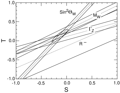
FIG. 1.: Fit to $S$ and $T$ from electroweak observables, with $M_{H}^{\rm ref}=500\,$GeV and $m_{t}^{\rm ref}=175\,$GeV.

We determine the physically allowed region of $S$-$T$ space from a $\chi^{2}$ fit to fourteen precisely measured electroweak observables. Each observable ${\cal O}_{i}$ is represented by a four-parameter linearized function,

$${\cal O}_{i} = {\cal O}_{i}^{\rm ref}+s_{i}S+t_{i}T+x_{i}(\alpha_{s}-\alpha_{s}^{\rm ref})$$ (14)

$$\mbox{}+y_{i}(\Delta\alpha^{5}_{had}-\Delta\alpha^{5}_{\rm ref})\,,$$

where ${\cal O}_{i}^{\rm ref}$ is the standard model value of the observable at the reference values of top quark and Higgs bosn masses. The strong coupling $\alpha_{s}$ is evaluated at the scale $M_{Z}$; we take $\alpha_{s}^{\rm ref}=0.12$ as the corresponding reference point. In this expression, $\Delta\alpha^{5}_{had}$ is the five-flavor, hadronic portion of the vacuum polarization correction to the electromagnetic coupling constant at the scale $M_{Z}$, and $\Delta\alpha^{5}_{\rm ref}=277.5\times 10^{-4}$ is its reference point. The coefficients $s_{i}$ and $t_{i}$ are computed from the standard model [2]. The coefficients $x_{i}$, $y_{i}$ and the reference values $O_{i}^{\rm ref}$ are computed using the ZFITTER 6.11 computer code [7]. All coefficients are insensitive to the choice of the reference points.

The fourteen observables are the width $\Gamma_{Z}$ of the $Z$ boson [8]; the $e^{+}e^{-}$ pole cross section of the $Z$ [8]; the ratio of the hadronic and leptonic partial widths of the $Z$ [8]; the $Z$-pole forward-backward asymmetries for final state leptons, $b$ quarks, and $c$ quarks [8]; $Z$-pole left-right coupling asymmetries for electrons and $\tau$ leptons as determined from final-state $\tau$ polarization measurements [8]; the $Z$-pole hadronic charge asymmetry [8]; the left-right cross section asymmetry for $Z$ production [8]; the mass $M_{W}$ of the $W$ boson [8]; $R_{-}$, a quantity constructed from the ratios of neutral- and charged-current $\nu$ and $\bar{\nu}$ cross sections [9]; the weak charge of the Cesium nucleus [10]; and the weak charge of the Thallium nucleus [11]. The fit is performed with $\Delta\alpha^{5}_{had}$ constrained to the value $(277.5\pm 1.7)\times 10^{-4}$, as determined by a recent analysis [12]. The $\chi^{2}$ weight matrix includes correlated errors for the LEP $Z$ lineshape parameters. The resulting two-dimensional 68.3% confidence region in $S$-$T$ space is shown in Fig 1 for the reference point $(m_{t}^{\rm ref},M_{H}^{\rm ref})=(175,500)\,$GeV. The one-dimensional 68% confidence intervals for the parameters are

$$S=-0.13\pm 0.10\,,\qquad T=0.13\pm 0.11\,,$$ (15)

$$\alpha_{s}(M_{Z})=0.119\pm 0.003\,,$$ (16)

$$\Delta\alpha^{5}_{had}(M_{Z})=(277.6\pm 1.7)\times 10^{-4}\,.$$ (17)

Note that the $S$ and $T$ confidence regions (one- and two-dimensional) implicitly incorporate the uncertainties resulting from the imprecise knowledge of $\alpha_{s}(M_{Z})$ and $\Delta\alpha^{5}_{had}(M_{Z})$.

To test the consistency of our approach, we perform a chi-square fit of the measured values of $S$ and $T$ to the standard model functions $S(m_{t},M_{H};m_{t}^{\rm ref},M_{H}^{\rm ref})$ and $T(m_{t},M_{H};m_{t}^{\rm ref},M_{H}^{\rm ref})$, which are calculated with ZFITTER 6.11. The $\chi^{2}$ weight matrix is obtained from the inverse of the $S$-$T$ error matrix. We add an additional term to the $\chi^{2}$ function to include a constraint on the top quark mass [13], $m_{t}=174.3\pm 5.1$ GeV. We then compare the result of this fit with that of a direct fit to the standard model using the same fourteen observables with the same constraints. The standard model fit yields a central value for $M_{H}$ of 106.3 GeV and a 95% upper limit of 228.5 GeV. The $S$-$T$ fit yields very consistent values of 107.4 GeV and 228.8 GeV, respectively.

In what follows, we use a similar procedure to derive confidence intervals for the parameters $S_{0}$, $T_{0}$, and $\Lambda$, which characterize the alternative electroweak symmetry breaking sector. The measured values of $S$ and $T$ are fit to the functions defined in equations (12), with the same reference masses as above. In addition, the same $m_{t}$-constraining term is added to the $\chi^{2}$ function.

Of course, it is not possible to determine all three of $S_{0}$, $T_{0}$ and $\Lambda$ using just two measurements. Indeed, for any fixed $\Lambda$, it is always possible to adjust the matching coefficients $S_{0}$ and $T_{0}$ to fit the low energy data. However, the situation $S\ll S_{0}$ and $T\ll T_{0}$ would be unnatural, since it would suggest finely tuned cancelations in equations (5). Indeed, there is no reason to expect any correlation between chiral lagrangian parameters generated directly at the scale $\Lambda$ and logarithmic radiative corrections generated in running the theory from $\Lambda$ down to $M_{Z}$. We will see that even for $\Lambda\approx 3\,$TeV, no such tuning is required.

The result of our fit is shown in Figure 2. We plot the allowed region for $S_{0}$ and $T_{0}$ for $\Lambda=(3,2,1,0.5,0.1)\,$TeV. The $\Lambda=100\,$GeV point is shown, although our chiral Lagrangian description is not valid for such a low cutoff. The 68% and 95% C.L. ellipses are shown for $\Lambda=3\,$TeV; the fit yields the central values $(S_{0},T_{0})=(-0.27,0.46)$ and the 68% C.L. ranges

$$-0.37<S_{0}<-0.17\,,\qquad 0.34<T_{0}<0.58\,,$$ (18)

For smaller $\Lambda$, the central values for $S_{0}$ and $T_{0}$ become smaller, as shown in Fig. 2 while the error ellipse retains its size and orientation.

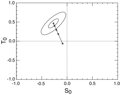
FIG. 2.: Fit to $S_{0}$ and $T_{0}$ from electroweak observables, for $\Lambda=(3,2,1,0.5,0.1)\,$TeV. Both 68% and 95% C.L. ellipses are shown for $\Lambda=3\,$TeV.

From the relation (6) between $(S_{0},T_{0})$ and $(a_{1},b_{1})$, we see that chiral lagrangian coefficients of order one or smaller are needed to fit the precision data, for all reasonable values of $\Lambda$. As a measure of the tuning which is required to fit the data, we compute the ratio of the constant term to the logarithm in equations (5); the deviation of this ratio from one is an indication of the degree to which the each constant must be adjusted to cancel the logarithm and fit the data at $M_{Z}$. Taking the central values $(a_{1},b_{1})=(0.85,1.11)$ from the fit at $\Lambda=3\,$TeV, we find a ratio of 1.4 for $S$ and 0.85 for $T$. Even without including the experimental uncertainties, we see that no significant tuning of $a_{1}$ and $b_{1}$ is required.

IV Conclusion

Precision electroweak measurements place a strong upper limit on about 230 GeV on the mass of the Higgs boson in the context of the standard model of particle physics. In this letter we have seen that these measurements do not rule out alternative theories. Indeed, we find that they permit strongly interacting theories with scales as high as 3 TeV.

Nevertheless, we have seen that precision measurements place significant constraints on these alternative theories. They constrain the parameters $a_{1}$ and $b_{1}$ to be of order unity, and for $\Lambda\gtrsim 1\,$ TeV, they completely fix their signs. It is, of course, an urgent and open question to determine whether a reasonable model can be constructed with these parameters. For example, it has previously been observed that it is difficult to obtain $a_{1}>0$ in naive technicolor theories [2]. In such models, $S$ receives a small positive contribution of approximately 0.1 for each weak doublet in the fundamental theory.

More generally, we would argue that the data disfavor models in which fermion masses are generated directly by the electroweak symmetry breaking dynamics. Fermion masses arise from interactions of the form

$$\Phi_{U}^{ij}\,\overline{Q}_{L}^{i}u_{R}^{j}+\Phi_{D}^{ij}\,\overline{Q}_{L}^{i}d_{R}^{j}+\Phi^{ij}_{L}\,\overline{L}_{L}^{i}e_{R}^{j}\,$$ (19)

where $i,j=1,2,3$ are flavor indices and $\Phi_{a}^{ij}$, $a=U,D,L$, are (possibly composite) fields which assume nonzero vacuum expectation values. In the standard model, $\Phi_{U}^{ij}=\lambda_{U}^{ij}\Phi$, $\Phi_{D}^{ij}=\lambda_{D}^{ij}\Phi^{*}$ and $\Phi_{L}^{ij}=\lambda_{L}^{ij}\Phi$, where $\Phi$ is the single Higgs boson and the $\lambda_{a}^{ij}$ are 27 Yukawa couplings which break the $U(3)^{5}$ flavor symmetry. In theories in which these symmetries are dynamically broken, the fields $\Phi_{a}^{ij}$ are dyanmical degrees of freedom that carry representations of the flavor symmetry group. When the $\Phi_{a}^{ij}$ are integrated out, they give a contribution to $a_{1}$ which includes a trace over a large number or fields. Generically, we expect the trace to be large: in the unrealistically minimal scenario in which the trace is 27 times the contribution of a single scalar, we find $|a_{1}|=27\times(5/72)=1.9$. A more realistic model would require significant cancelations to achieve the observed value of $a_{1}$.

J.B. would like to thank the Aspen Center for Physics for hospitality. This work was supported in part by the National Science Foundation under grants PHY–9404057 and PHY–9604893. Support for A.F. was also provided by the NSF under National Young Investigator Award PHY–9457916, by the DOE under Outstanding Junior Investigator Award DE–FG02–94ER40869, by the Research Corporation under the Cottrell Scholar program, and by the Alfred P.  Sloan Foundation.

Note added. After this work was completed, we bacame aware of Ref. [14]. In this paper the authors claim that the upper bound on $\Lambda$ is very close to the upper bound on $M_{H}$ in the standard model. The authors of this paper neglect $a_{1}$ and $b_{1}$, so their bound holds in the class of models where $a_{1}$ and $b_{1}$ are near zero.

REFERENCES

- [1] M. Swartz, presentation at the 1999 Lepton-Photon Symposium.
- [2] M.E. Peskin and T. Takeuchi, Phys. Rev. Lett. 65, 964 (1990); Phys. Rev. D 46, 381 (1992).
- [3] C. Kolda and L. Hall, hep-ph/9904236; R. Barbieri and A. Strumia, hep-ph/9905281; R.S. Chivukula and N. Evans, hep-ph/9907414.
- [4] T. Appelquist and C. Bernard, Phys. Rev. D22, 300 (1980); A.C. Longhitano, Nucl. Phys. B188, 118 (1981); Phys. Rev. D22, 1166 (1980); A. Dobado and M.J. Herrero, Phys. Lett B228, 495 (1989); B233, 505 (1989); J. Donoghue and C. Ramirez, Phys. Lett. B234, 361 (1990); S. Dawson and G. Valencia, Nucl. Phys. B352, 27 (1991); A. Dobado, D. Espriu and M.J. Herrero, Phys. Lett. B255, 405 (1991); A. Dobado, M.J. Herrero and J. Terron, Z. Phys. C50, 205 (1991); J. Bagger, S. Dawson and G. Valencia, Nucl. Phys. B399, 364 (1993).
- [5] M.J. Herrero and E. Ruiz Morales; Nucl. Phys. B418, 431 (1994); B437, 319 (1995); S. Dittmaier and C. Grosse-Knetter, Nucl. Phys. B459, 497 (1996).
- [6] M. Golden and L. Randall, Nucl. Phys. B361, 3 (1991).
- [7] D. Bardin, et. al., DESY preprint 99-070, 1999.
- [8] J. Mnich, presentation at the International Europhysics Conference on High Energy Physics, Tampere, Finland, July 1999.
- [9] K.S. McFarland et al., hep-ex/9806013.
- [10] S.C. Bennett and C.E. Wieman, Phys. Rev. Lett. 82, 2484 (1999).
- [11] P.A. Vetter, et al., Phys. Rev. Lett. 74, 2658 (1995); N.H. Edwards, et al., Phys. Rev. Lett. 74, 2654 (1995).
- [12] J.H. Kuhn and M. Steinhauser, Phys. Lett. B437, 425 (1998).
- [13] F. Abe et al., Phys. Rev. Lett. 82, 271 (1999); D. Abbot et al., Phys. Rev. D58, 052001 (1998).
- [14] B. Kniehl and A. Sirlin, hep-ph/9907293.