$K_{L}^{0}\rightarrow\pi^{+}\pi^{-}e^{+}e^{-}$ in Chiral Perturbation Theory

Kaon decays continue to provide invaluable information about the approximate discrete symmetries of nature. CP-violation in $K_{L}^{0}\rightarrow\pi\pi$[1], originating in the $K^{0}-\overline{K}^{0}$ mass matrix, was discovered nearly forty years ago and direct CP-violation in K-decays has been unambiguously established[2, 3, 4], through a recent remeasurement of ${\rm Re}\left(\epsilon^{\prime}/\epsilon\right)=(28.0\pm 3.0\pm 2.8)\times 10^{-4}$ by the KTeV collaboration[4]. KTeV has also observed and studied[5] the rare decay $K_{L}^{0}\rightarrow\pi^{+}\pi^{-}e^{+}e^{-}$. A large CP-violating asymmetry, $B_{\rm CP}=13.6\pm 2.5\pm 1.2\ \%$, constructed from the final state particles was measured[5], consistent with theoretical predictions[6, 7, 8, 9]. This decay is dominated by a one-photon intermediate state, $K_{L}^{0}\rightarrow\pi^{+}\pi^{-}\gamma^{*}\rightarrow\pi^{+}\pi^{-}e^{+}e^{-}$ and $B_{\rm CP}$ receives a sizable strong interaction enhancement.

A long standing problem in better understanding K-decays and a roadblock to more precisely constraining the standard model of electroweak interactions or uncovering new physics is our present inability to compute the hadronic matrix elements of most electroweak operators to high precision. The lattice provides the only direct method with which to determine these matrix elements, however, it is presently far from being able to compute matrix elements between multi-hadronic initial and final states. Chiral perturbation theory, $\chi PT$, is a framework in which the low-energy strong interactions of the lowest-lying pseudo-Goldstone bosons can be treated in perturbation theory. The external momentum and the light quark mass matrix are treated as small expansion parameters when normalized to the chiral symmetry breaking scale, $\Lambda_{\chi}\sim 1~{}{\rm GeV}$. This article presents the $\chi PT$ analysis of $K_{L}^{0}\rightarrow\pi^{+}\pi^{-}e^{+}e^{-}$, focusing entirely on the one-photon intermediate state, as shown in fig. (1).

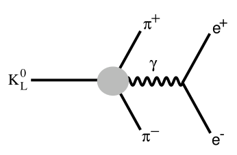
Figure 1: The one-photon intermediate state dominates $K_{L}^{0}\rightarrow\pi^{+}\pi^{-}e^{+}e^{-}$. The solid circle denotes the $K_{L}^{0}\rightarrow\pi^{+}\pi^{-}\gamma^{*}$ vertex.

The matrix element for $K_{L}^{0}\rightarrow\pi^{+}\pi^{-}e^{+}e^{-}$, assuming CPT-invariance, is written in terms of three form factors $G$, $F_{+}$ and $F_{-}$,

$${\cal M} = {s_{1}\ G_{F}\ \alpha\over 4\pi\ f\ q^{2}}\left[\ i\ G\ \varepsilon_{\mu\lambda\rho\sigma}\ p_{+}^{\lambda}\ p_{-}^{\rho}\ q^{\sigma}\ +\ F_{+}\ p_{+,\mu}\ +\ F_{-}\ p_{-,\mu}\ \right]$$ (1)

$$\overline{u}(k_{-})\gamma^{\mu}\ v(k_{+})\ \ \ ,$$

where $k_{+,-}$ are the positron and electron momenta respectively, $q=k_{+}+k_{-}$ is the photon momentum and $p_{+,-}$ are the $\pi^{+,-}$ momenta respectively. $G_{F}$ is Fermi’s coupling constant, $s_{1}$ is the sine of the Cabbibo angle, $f$ is the pion decay constant, and $\alpha$ is the electromagnetic fine structure constant. The form factors are functions of hadronic kinematic invariants, e.g. $F_{+}=F_{+}(q^{2},q\cdot p_{+},q\cdot p_{-})$. The smallness of ${\rm Re}\left(\epsilon^{\prime}/\epsilon\right)$ suggests that to a very good approximation direct CP violation that may contribute to this decay can be neglected. For our purposes the only CP violation that will enter into this decay is due to $\epsilon$, indirect CP violation introduced by the $K^{0}_{L}$ wavefunction. In terms of the eigenstates of CP, $K_{1,2}$, the $K^{0}_{L}$ wavefunction is

$$|K_{L}^{0}\rangle = |K_{2}\rangle\ +\ \epsilon|K_{1}\rangle$$

$$|K_{1}\rangle = {1\over\sqrt{2}}\left[\ |K^{0}\rangle\ -\ |\overline{K}^{0}\rangle\ \right]\ \ ,\ \ |K_{2}\rangle\ =\ {1\over\sqrt{2}}\left[\ |K^{0}\rangle\ +\ |\overline{K}^{0}\rangle\ \right]\ \ \ ,$$ (2)

where $CP|K_{1}\rangle=+|K_{1}\rangle$, $CP|K_{2}\rangle=-|K_{2}\rangle$ and $\epsilon=0.0023\ e^{i44^{o}}$. As direct CP violation is being neglected it is convenient to determine the contributions to $G$, $F_{+}$ and $F_{-}$ from $K_{1}$ and $K_{2}$ independently as the two contributions do not interfere in the total decay rate, $\Gamma$, or differential decay rate $d\Gamma/dq^{2}$. The CP-odd component of the $K_{L}^{0}$ wavefunction, $K_{2}$, gives contributions to the form factors with symmetry properties $G\rightarrow+G$, and $F_{\pm}\rightarrow+F_{\mp}$ under interchange $p_{\pm}\rightarrow p_{\mp}$, while the contributions from the CP-even component of the $K_{L}^{0}$ wavefunction, $K_{1}$, have symmetry properties $F_{\pm}\rightarrow-F_{\mp}$ under interchange $p_{\pm}\rightarrow p_{\mp}$ (where it is understood that the interchange $p_{\pm}\rightarrow p_{\mp}$ also occurs for the arguments of the form factors).

The lagrange density that describes the leading order strong and $\Delta s=1$ weak interactions of the lowest-lying octet of pseudo-Goldstone bosons is

$${\cal L} = {f^{2}\over 8}{\rm Tr}\left[D^{\mu}\Sigma D_{\mu}\Sigma^{\dagger}\right]\ +\ \lambda{\rm Tr}\left[m_{q}\ \Sigma\ +\ {\rm h.c.}\right]$$ (3)

$$+ g_{8}\ {G_{F}s_{1}f^{4}\over 4\sqrt{2}}\left(\left[D^{\mu}\Sigma D_{\mu}\Sigma^{\dagger}H_{w}\right]\ +\ {\rm h.c.}\right)\ \ \ ,$$

where

$$\Sigma = Exp\left[{2i\over f_{\pi}}\left(\matrix{{1\over\sqrt{2}}\pi^{0}+{1\over\sqrt{6}}\eta&\pi^{+}&K^{+}\cr\pi^{-}&-{1\over\sqrt{2}}\pi^{0}+{1\over\sqrt{6}}\eta&{1\over\sqrt{2}}K_{2}^{0}+{1\over\sqrt{2}}K_{1}^{0}\cr K^{-}&{1\over\sqrt{2}}K_{2}^{0}-{1\over\sqrt{2}}K_{1}^{0}&-{2\over\sqrt{6}}\eta}\right)\right]\ \ \ ,$$ (4)

and $H_{w}$ is a $3\times 3$ matrix with a “1” in the $(1,3)$ entry, inducing a $s\rightarrow u$ transition. Octet dominance ($\Delta I={1\over 2}$) has been assumed and thus contributions from the ${\bf 27}$ component of the $\Delta s=1$ hamiltonian have been neglected. The constant $|g_{8}|=5.1$ is fit to the amplitude for $K\rightarrow\pi\pi(I=0)$.

In computing observables in $\chi PT$, the external momentum and quark masses are expansion parameters in which the form factors are expanded, e.g. $G=G^{(1)}+G^{(2)}+G^{(3)}+...$. The form factor $G^{(r)}$ is associated with a contribution of order $Q^{2r-1}$, where $Q=p,m$, the external momenta or meson mass. The same expansion and notation is used for the $F_{\pm}$ form factors. Unlike the contributions from the $K_{2}$ component, contributions from the $K_{1}$ component are suppressed by a factor of $\epsilon$. However, the leading order contribution to $K_{L}^{0}\rightarrow\pi^{+}\pi^{-}\gamma^{*}$, $r=1$, is from tree-graphs involving the $K_{1}$ component, as shown in fig. (2).

Figure 2: The leading order contribution to $K_{L}^{0}\rightarrow\pi^{+}\pi^{-}\gamma^{*}$ in $\chi PT$. A solid square denotes a weak interaction. Only the $K_{1}$ component of the $K_{L}^{0}$ wavefunction can contribute at tree-level and this contribution is suppressed by a factor of $\epsilon$.

A simple calculation yields

$$F_{+,1}^{(1)} = -\epsilon\ g_{8}{32f_{\pi}^{2}(m_{K}^{2}-m_{\pi}^{2})\pi^{2}\over q^{2}+2q\cdot p_{+}}\ \ \ ,\ \ \ F_{-,1}^{(1)}\ =\ +\epsilon\ g_{8}{32f_{\pi}^{2}(m_{K}^{2}-m_{\pi}^{2})\pi^{2}\over q^{2}+2q\cdot p_{-}}\ \ \ ,$$ (5)

and $G^{(1)}\ =\ 0$, which has the correct symmetry under $p_{\pm}\rightarrow p_{\mp}$ as discussed previously. The subscript on the $F_{\pm}$ form factors indicate that the contribution comes from the $K_{1}$ component. As all constants appearing in eq. (5) are determined by other processes, this is a parameter free leading order prediction. Final state strong interactions that contribute to $F_{\pm,1}$ are important for CP-violating asymmetries such as $B_{\rm CP}$. The leading final state interactions associated with $F_{\pm,1}$ are generated by graphs shown in fig. (3).

Figure 3: The leading final-state interactions in $K_{1}\rightarrow\pi^{+}\pi^{-}\gamma^{*}$. A solid square denotes a weak interaction and a solid circle denotes a strong interaction. These contribution are proportional to $\epsilon$.

Retaining only the imaginary parts of the graphs, naively enhanced by factors of $\pi$ over the real parts, we have

$${\rm Im}\left[F_{+,1}^{(2)}\right] = -g_{8}\ \pi\epsilon\ {\left(m_{K}^{2}-m_{\pi}^{2}\right)\left(4m_{K}^{2}-2m_{\pi}^{2}\right)\over q^{2}+2q\cdot p_{+}}\sqrt{1-{4m_{\pi}^{2}\over m_{K}^{2}}}\ \ \ ,$$ (6)

which is the leading term in building up $e^{i\delta_{0}}$, where $\delta_{0}$ is the $I=J=0$ $\pi\pi$ phase shift evaluated at $s=m_{K}^{2}$.

Decay of the $K_{2}$ component is described by both the $G$ and $F_{\pm,2}$ form factors starting at $r=2$, as can be seen from eq. (1). At this order in $\chi PT$, $G^{(2)}$ is a constant that must be determined from data. The M1 fraction of the decay rate for $K_{L}^{0}\rightarrow\pi^{+}\pi^{-}\gamma$ is reproduced if $G^{(2)}=39.3$, where higher order (momentum dependent) contributions have been neglected, and $G^{(2)}$ is real. The dalitz plot for $K_{L}^{0}\rightarrow\pi^{+}\pi^{-}\gamma$ indicates that there is non-negligible momentum dependence in $G$, and therefore higher order terms will be important[10, 11]. This introduces an uncertainty into the prediction of differential rates and CP-violating asymmetries at the order to which we are working. At $r=3$ there are contributions, not only from loop diagrams, but also from higher order weak interactions and the Wess-Zumino term. However, as before we are able to compute the leading contribution to the imaginary part of $G$, that go to build up the final state interactions, $e^{i\delta_{1}}$, where $\delta_{1}$ is the phase shift for $\pi\pi$ scattering in the $I=J=1$ channel. It is found that

$${\rm Im}\left[G^{(3)}\right] = G^{(2)}\ {s\over 48\pi f^{2}}\left[1-{4m_{\pi}^{2}\over s}\right]^{3/2}\ \ \ ,$$ (7)

where $s$ is the invariant mass of the $\pi^{+}\pi^{-}$ system.

The $F_{\pm,2}$ form factors do not arise only from the charge radius of the $K^{0}$ as was assumed in the analyses of [6, 7]. In fact, the $K^{0}$ charge radius is one of several different types of one-loop graphs arising at $r=2$ that give rise to $q^{2}$-dependence in the $F_{\pm,2}$. The diagrams giving contributions from the charge radii of the $K^{0}$ and the $\pi^{\pm}$ are shown in fig. (4).

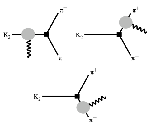
Figure 4: Contributions to $K_{L}^{0}\rightarrow\pi^{+}\pi^{-}\gamma^{*}$ from the $K$ and $\pi$ charge radii. The solid square denotes a weak interaction and the lightly shaded circle denotes the sum of one-loop graphs and counterterms that form the charge radius of either the $K$ or the $\pi$.

The sum of the one-loop diagrams contributing to the $K^{0}$ charge radius is finite, while those contributing to the $\pi$ charge radius are divergent and require the counterterm

$${\cal L} = -i\ \lambda_{\rm cr}{e\over 16\pi^{2}}\ F^{\mu\nu}\ Tr\left[Q\left(D_{\mu}\Sigma D_{\nu}\Sigma^{\dagger}+D_{\mu}\Sigma^{\dagger}D_{\nu}\Sigma\right)\right]\ \ \ ,$$ (8)

where $Q$ is the light-quark electromagnetic charge matrix, and $F^{\mu\nu}$ is the electromagnetic field strength tensor. The coefficient $\lambda_{\rm cr}=-0.91\pm 0.06$ has been determined from measurements of the $\pi$ charge radius.

Diagrams that are not charge radius type contributions are shown in fig. (5).

,

,

Figure 5: One-loop contributions to $K_{2}\rightarrow\pi^{+}\pi^{-}\gamma^{*}$ from diagrams that do not contribute to the charge radius of the $K$ or $\pi$. A solid square denotes a weak interaction and a solid circle denotes a strong interaction.

Analytic expressions for the diagrams shown in fig. (5), given in [8, 9], are somewhat lengthy and we do not present them here. The sum of the graphs in fig. (5) is not finite and the counterterms that enter at this order are described by the lagrange density[12]

$${\cal L}\ =\ i\ g_{8}\ {G_{F}\ s_{1}\ e\ f_{\pi}^{2}\over 16\sqrt{2}\pi^{2}}\left[\ a_{1}\ F^{\mu\nu}\ {\rm Tr}\left[QH_{w}(\Sigma D_{\mu}\Sigma^{+})(\Sigma D_{\nu}\Sigma^{\dagger})\right]\right.$$ (9)

$$\left.+a_{2}\ F^{\mu\nu}\ {\rm Tr}\left[Q(\Sigma D_{\mu}\Sigma^{\dagger})H_{w}(\Sigma D_{\nu}\Sigma^{\dagger})\right]\right.$$

$$\left.+a_{3}\ F^{\mu\nu}\ {\rm Tr}\left[H_{w}[Q,\Sigma]D_{\mu}\Sigma^{\dagger}\Sigma D_{\nu}\Sigma^{\dagger}-H_{w}D_{\mu}\Sigma D_{\nu}\Sigma^{\dagger}\Sigma[\Sigma^{\dagger},Q]\right]\right.$$

$$\left.+a_{4}\ F^{\mu\nu}\ {\rm Tr}\left[H_{w}\Sigma D_{\mu}\Sigma^{\dagger}[Q,\Sigma]D_{\nu}\Sigma^{\dagger}\right]\ \right]+h.c.\ \ \ ,$$

where the constants $a_{1,2,3,4}$ must be determined from data. The combination of counterterms that contributes to $K_{L}^{0}\rightarrow\pi^{+}\pi^{-}\gamma^{*}$ is

$$w = a_{3}-a_{4}+{1\over 6}(a_{1}+2a_{2})+\lambda_{\rm cr}\ \ \ ,$$ (10)

while the combination that contributes to $K^{+}\rightarrow\pi^{+}e^{+}e^{-}$ is

$$w_{+}={2\over 3}(a_{1}+2a_{2})-4\lambda_{\rm cr}-{1\over 6}\log\left({m_{K}^{2}\ m_{\pi}^{2}\over\mu^{4}}\right)+{1\over 3}\ \ \ .$$ (11)

One has the choice to write the $F_{\pm,2}$ in terms of $w$, or to use the known values of $\lambda_{\rm cr}$ and $a_{1}+2a_{2}$ and define the finite, $\mu$-independent combination $w_{L}=a_{3}-a_{4}$[8]. The value of $w_{L}$ can be determined from the rate for $K_{L}^{0}\rightarrow\pi^{+}\pi^{-}e^{+}e^{-}$.

The differential decay rate is the incoherent sum of the rates from the three form factors,

$${d\Gamma\over dq^{2}} = {d\Gamma_{G}\over dq^{2}}\ +\ {d\Gamma_{F_{1}}\over dq^{2}}\ +\ {d\Gamma_{F_{2}}\over dq^{2}}\ \ \ \ ,$$ (12)

due to the symmetry properties of the amplitudes. In fig. (6)

Figure 6: The branching fraction ${1\over\Gamma_{\rm tot}}{d\Gamma\over dy}$ verses $y$, where $y=\sqrt{q^{2}}/(m_{K}-2m_{\pi})$. The dot-dashed, dashed and dotted curves are the contributions from $F_{\pm,1}$, $G$ and $F_{\pm,2}$ respectively, while the solid curve is the sum of the contributions. The three different plots correspond to the counterterm $w_{L}$ taking the values $0.40,0.47$ and $0.50$ respectively.

we have shown the differential branching fraction ${1\over\Gamma_{\rm tot}}{d\Gamma\over dy}$, where $y=\sqrt{q^{2}}/(m_{K}-2m_{\pi})$, for different values of $w_{L}$, given the central value of $w_{+}=0.89$[13] and the central value of $\lambda_{\rm cr}=-0.91$. The contribution to the differential rate from $F_{\pm,2}$ vanishes as $q^{2}\rightarrow 0$, but clearly dominates the high $q^{2}$ region (for most values of $w_{L}$). Except for the $q^{2}\rightarrow 0$ region, the contribution from $G$ dominates over the contribution from $F_{\pm,1}$. It is clear that in order to determine $w_{L}$ a relatively high cut on the $e^{+}e^{-}$ invariant mass must be made. To emphasize this point, the branching fraction for $K_{L}^{0}\rightarrow\pi^{+}\pi^{-}e^{+}e^{-}$ with a cut of $q^{2}_{\rm cut}>(2~{}{\rm MeV})^{2}$ is (using the parameter values already discussed)

$${\rm Br} = \left(16.1\ +\ 10.7\ +\ \left[\ 3.7\ -\ 3.5\ w_{L}\ +\ 0.8\ w_{L}^{2}\ \right]\right)\ 10^{-8}\ \ \ ,$$ (13)

where the first contribution is from $G$, the second is from $F_{1}$ and the third is from $F_{2}$. In contrast, the branching fraction with a cut of $q^{2}_{\rm cut}>(80~{}{\rm MeV})^{2}$ is

$${\rm Br} = \left(0.60\ +\ 0.07\ +\ \left[\ 1.9\ -\ 1.8\ w_{L}\ +\ 0.4\ w_{L}^{2}\ \right]\right)\ 10^{-8}\ \ \ .$$ (14)

With the presently available branching fraction of ${\rm Br}=(3.32\pm 0.14\pm 0.28)\times 10^{-7}$ from KTeV[5], which has a $q^{2}_{\rm cut}>(2~{}{\rm MeV})^{2}$ cut, $w_{L}=4.7\pm 0.7$ or $-0.6\pm 0.7$, but these values depend sensitively upon $G^{(2)}$ and $F_{\pm,1}$ for obvious reasons. Only an analysis of the entire differential spectrum, or the shape of the $\pi^{+}\pi^{-}$ invariant mass distribution will place more stringent bounds on $w_{L}$.

One of the most exciting aspects of $K_{L}^{0}\rightarrow\pi^{+}\pi^{-}e^{+}e^{-}$ is the large value of $B_{\rm CP}$ that is predicted[6, 7, 8, 9] and also recently observed by KTeV[5]. $B_{\rm CP}$ is defined to be

$$B_{\rm CP} = \langle Sign\left[\sin\phi\cos\phi\right]\rangle$$ (15)

$$= \langle Sign\left[\left(n_{e}\cdot n_{\pi}\right)n_{e}\times n_{\pi}\cdot\left({p_{+}+p_{-}\over|p_{+}+p_{-}|}\right)\right]\rangle\ \ \ ,$$

where $\phi$ is the Pais-Trieman variable depicted in fig. (7),

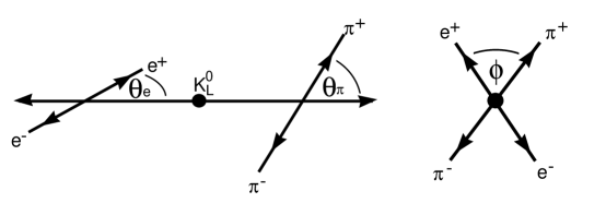
Figure 7: Definition of the Pais-Trieman variables, $\phi$, $\theta_{e}$ and $\theta_{\pi}$.

$n_{e}$ is the normal to the plane formed by the momenta of the $e^{+}e^{-}$ pair and $n_{\pi}$ is the normal to the plane formed by the momenta of the $\pi^{+}\pi^{-}$ pairs. It is integrated over the momenta of the final state particles with any specified cuts. The integrand that contributes to $B_{\rm CP}$ is proportional to the combination

$$Im\left[\ G\ \left(F_{+,1}-F_{-,1}\right)^{*}\right] = Im\left[\ G^{(2)}\ \left(F_{+,1}^{(1)}-F_{-,1}^{(1)}\right)^{*}\ +\ \ G^{(2)}\ \left(F_{+,1}^{(2)}-F_{-,1}^{(2)}\right)^{*}\right.$$ (16)

$$\left.\ \ +\ G^{(3)}\ \left(F_{+,1}^{(1)}-F_{-,1}^{(1)}\right)^{*}\ \ +\ \ ...\right]\ \ \ .$$

The contribution from ${\rm Re}\left[G^{(3)}\right]$ has not been computed, and therefore this does not constitute a complete computation of $B_{\rm CP}$ to next-to-leading order. However, the omitted contribution is expected to be small[8, 9]. With a cut of $q^{2}_{\rm cut}>(2~{}{\rm MeV})^{2}$ this asymmetry is found to be[8, 9]

$$B_{\rm CP} = 9.2\%\ +\ 4.2\ \%\ +\ ...\ =\ 13.4\ \%\ \ \ ,$$ (17)

with an uncertainty estimated to be of order $\sim 2\%$ based on the difference between the leading and next-to-leading order contributions. This is in complete agreement with the recent KTeV[5] observation of $B_{\rm CP}=13.6\pm 2.5\pm 1.2\ \%$ for this invariant mass cut, and consistent with the calculations of [6, 7]. The next-to-leading order contribution of $4.3\%$ is from the final-state interactions associated with $F_{\pm,1}$. It is important to note that $F_{\pm,2}$ does not contribute to $B_{\rm CP}$, and hence the uncertainty in determining $w_{L}$ does not impact this discussion. As emphasized by Sehgal[14], good agreement between theory and the current experimental value of $B_{\rm CP}$ is obtained within the context of the standard model, with CP-violation from $\epsilon$ and CPT-conservation. Recent discussions of the implication of this observation for T-violating interactions can be found in [15, 16]. While reversing the momenta of the final state particles does change the sign of $B_{\rm CP}$ (it is T-odd), the initial and final states in the decay have not been interchanged. Therefore, a direct connection to T-violating interactions is absent.

In conclusion, I have presented a systematic analysis of the decay $K_{L}^{0}\rightarrow\pi^{+}\pi^{-}e^{+}e^{-}$ in chiral perturbation up to next-to-leading order. This analysis differs from that of [6, 7] in the form of the $K_{L}^{0}\rightarrow\pi^{+}\pi^{-}\gamma^{*}$ dependence upon $q^{2}$. The size of this contribution is determined by a counterterm, $w_{L}$, that presently is only loosely constrained, but could be determined from the existing KTeV data with appropriate kinematic cuts. The large value of the CP-asymmetry, $B_{\rm CP}$, that was predicted to arise naturally from $\epsilon$ has been confirmed by the KTeV collaboration[5].

I would like to thank Jon Rosner and Bruce Winstein for putting together a very stimulating workshop. This work is supported in part by Department of Energy Grant DE-FG03-97ER41014.

References

[1] J. H. Christenson, J. W. Cronin, V. L. Fitch and
R. Turlay,
Phys. Rev. Lett.13, 138 (1964).
[2] G. Barr et al, (NA31 Collaboration),
Phys. Lett.B317, 233 (1993).
[3] L. K. Gibbons et al,
(E731 Collaboration),
Phys. Rev. Lett.70, 1203 (1993).
[4] A. Alavi-Harati et al, (KTeV Collaboration),
hep-ex/9905060.
[5] J. Adams et al, (KTeV Collaboration),
Phys. Rev. Lett.80, 4123 (1998);
A. Ledovskoy, (KTeV Collaboration),
talk presented at this meeting.
[6] L. M. Sehgal and M. Wanninger,
Phys. Rev. D46, 1035 (1992);
Phys. Rev. D46, 5209 (1992)(E).
[7] P. Heiliger and L. M. Sehgal,
Phys. Rev. D48, 4146 (1993).
[8] J. K. Elwood, M. J. Savage and M. B. Wise,
Phys. Rev. D52, 5095 (1995);
Phys. Rev. D53, 2855 (1996)(E).
[9] J. K. Elwood, M. J. Savage, J. W. Walden
and M. B. Wise,
Phys. Rev. D53, 4078 (1996).
[10] G. Ecker, H. Neufeld and A. Pich,
Nucl. Phys.B413, 321 (1994).
[11] G. D’Ambrosio and J. Portoles,
Nucl. Phys. B533, 523 (1998).
[12] G. Ecker, J. Kambor and D. Wyler,
Nucl. Phys.B394, 101 (1993).
[13] G. Donaldson et al,
Phys. Rev. Lett.33, 554 (1974);
Phys. Rev. D14, 2839 (1976);
E. J. Ramberg et al, Phys. Rev. Lett.70, 2525 (1993).
[14]L. M. Sehgal, talk presented at this workshop.
[15] J. Ellis and N. E. Mavromatos, hep-ph/9903386.
[16]
L. Alvarez-Gaume, C. Kounnas, S. Lola and P. Pavlopoulos,
hep-ph/9903458.
,
,
,
,