Hard-thermal-loop Resummation
of the Free Energy of a Hot Quark-Gluon Plasma

Abstract

The quark contribution to the free energy of a hot quark-gluon plasma is calculated to leading order in hard-thermal-loop (HTL) perturbation theory. This method selectively resums higher order corrections associated with plasma effects, such as screening, quasiparticles, and Landau damping. Comparing to the weak-coupling expansion of QCD, the error in the one-loop HTL free energy is of order $\alpha_{s}$, but the large $\alpha_{s}^{3/2}$ correction from QCD plasma effects is included exactly.

I Introduction

Experimental data from ultrarelativistic heavy-ion collisions at RHIC will soon become available. In order to determine if a quark-gluon plasma has been created, a careful comparison of the predictions of hadronic models and QCD has to be made. It is therefore desirable to find a systematic way to calculate the thermodynamic properties and signatures of a quark-gluon plasma within QCD. Asymptotic freedom suggests that at sufficiently high temperatures a straightforward perturbative expansion should suffice. However, at experimentally accessible temperatures, perturbative QCD does not seem to be of any quantitative use [1-3]. The problem is evident in the free energy of the quark-gluon plasma. The weak-coupling expansion has been calculated through order $\alpha_{s}^{5/2}$ [1-3]. The successive approximations to the free energy show no sign of converging at temperatures that are relevant for heavy-ion collisions.

One possibility for improving the convergence of the perturbative predictions is to apply Padé approximants to the series in $\alpha_{s}^{1/2}$ [4], however, this technique can only be applied if several terms in the perturbation series are known. Another possibility is to use hard-thermal-loop (HTL) approximations within a self-consistent $\Phi$-derivable framework [5]. A third approach is to apply HTL perturbation theory [6], which is an extension of the resummation method of Braaten and Pisarski [7] into a systematic perturbative expansion. In two previous papers [6], we calculated the one-loop free energy of pure-glue QCD using HTL perturbation theory. Here we extend that calculation to include quarks, thus completing the calculation of the free energy of a hot quark-gluon plasma to leading order in HTL perturbation theory.

The paper is organized as follows. In the next section, we calculate the quark contribution to the free energy of a hot quark-gluon plasma at one loop in HTL perturbation theory. In section III, we carry out the high-temperature expansion of the free energy, and in section IV we take the low-temperature limit. In section V, we compare the one-loop HTL free energy with the weak-coupling expansion of QCD. We conclude in section VI. In the appendix, we have collected the integrals that are required in the calculations.

II Quark Contribution to HTL Free Energy

The one-loop HTL free energy for an $SU(N_{c})$ gauge theory with $N_{f}$ massless quarks is

$${\cal F}_{\rm HTL}=(N_{c}^{2}-1)\left[(d-1){\cal F}_{T}+{\cal F}_{L}\right]+N_{c}N_{f}{\cal F}_{q}+\Delta{\cal F}\,,$$ (1)

where ${\cal F}_{T}$ and ${\cal F}_{L}$ are the contributions to the free energy from transverse and longitudinal gluons, respectively, ${\cal F}_{q}$ is the contribution to the free energy from each flavor and color of the quarks, and $\Delta{\cal F}$ is a counterterm. The quark contribution is given by

$${\cal F}_{q} = -\hbox{$\sum$}\!\!\!\!\!\!\int_{K}\log\det[K\!\!\!\!/-\Sigma(K)]\,.$$ (2)

The sum-integral in (2) represents a dimensionally regularized integral over the momentum ${\bf k}$ and a sum over the Matsubara frequencies $\omega_{n}=(2n+1)\pi T$:

$$\hbox{$\sum$}\!\!\!\!\!\!\int_{K}\equiv T\sum_{n=-\infty}^{\infty}\mu^{3-d}\int{d^{d}k\over(2\pi)^{d}}\,.$$ (3)

The factor of $\mu^{3-d}$, where $\mu$ is a renormalization scale, ensures that the regularized free energy has the correct dimensions even for $d\neq 3$. The HTL quark self-energy in (2) is

$$\Sigma(K)={m_{q}^{2}\over 2k}\log{{{i\omega_{n}}+{k}\over{i\omega_{n}}-{k}}}\gamma_{0}+{m_{q}^{2}\over k}\left(1-{i\omega_{n}\over 2k}\log{{{i\omega_{n}}+{k}\over{i\omega_{n}}-{k}}}\right)\hat{\bf k}\cdot\mbox{\boldmath$\gamma$}\,,$$ (4)

where $\hat{\bf k}={\bf k}/k$ and $m_{q}$ is the thermal quark mass parameter [8].

We proceed to calculate the quark contribution to the HTL free energy. The inverse quark propagator can be written as

$$K\!\!\!\!/-\Sigma(K)=A_{0}(K)\gamma_{0}-A_{S}(K){\hat{\bf k}}\cdot\mbox{\boldmath$\gamma$}\,,$$ (5)

where

$$A_{0}(K) = i\omega_{n}-{m_{q}^{2}\over 2k}\log{{{i\omega_{n}}+{k}\over{i\omega_{n}}-{k}}}\,,$$ (6)

$$A_{S}(K) = k+{m_{q}^{2}\over k}\left(1-{i\omega_{n}\over 2k}\log{{{i\omega_{n}}+{k}\over{i\omega_{n}}-{k}}}\right)\,.$$ (7)

We can write the quark contribution (2) as

$${\cal F}_{q} = -2\hbox{$\sum$}\!\!\!\!\!\!\int_{K}\log(k^{2}+\omega_{n}^{2})-2\;\hbox{$\sum$}\!\!\!\!\!\!\int_{K}\log\left[{A_{S}^{2}-A_{0}^{2}\over k^{2}+\omega_{n}^{2}}\right]\,,$$ (8)

where we have separated out the free energy of an ideal gas of massless fermions. The first sum-integral in (8) can be evaluated analytically. In the second sum-integral, the sum over Matsubara frequencies can be expressed as a contour integral:

$${\cal F}_{q}=-{7\pi^{2}\over 180}T^{4}+2\int_{{\bf k}}\int_{C}{d\omega\over 2\pi i}\log\left[{(A_{0}-A_{S})(A_{0}+A_{S})\over\omega^{2}-k^{2}}\right]{1\over e^{\beta\omega}+1}\,,$$ (9)

where the contour $C$ encloses the points $\omega=i\omega_{n}$ along the imaginary axis in Fig. 1. We have introduced a condensed notation for the dimensionally regularized momentum integral:

$$\int_{\bf k}=\mu^{3-d}\int{d^{d}k\over(2\pi)^{d}}.$$ (10)

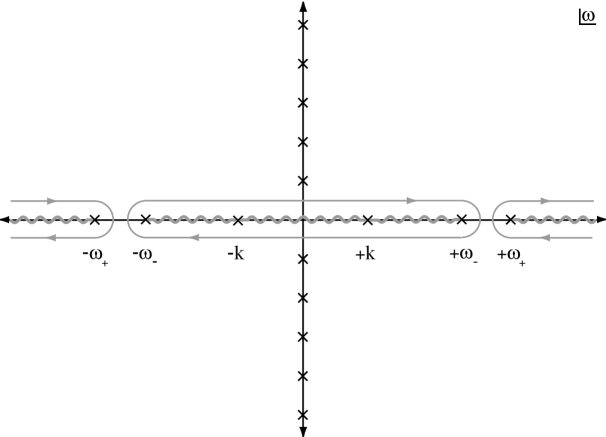
FIG. 1.: The quark contribution to the HTL free energy can be expressed as an integral over a contour $C$ that wraps around the branch cuts of $\log[(A_{0}^{2}-A_{S}^{2})/(\omega^{2}-k^{2})]$.

The integrand in (9) has logarithmic branch cuts that run from $-\infty$ to $-\omega_{+}$, from $-\omega_{-}$ to $\omega_{-}$, from $\omega_{+}$ to $+\infty$, and from $-k$ to $k$, where $\omega_{\pm}$ are the quasiparticle dispersion relations that satisfy $A_{0}\mp A_{S}=0$, or

$$0 = \omega_{\pm}\mp k-{m_{q}^{2}\over 2k}\left[\left(1\mp{\omega_{\pm}\over k}\right)\log{{{\omega_{\pm}}+{k}\over{\omega_{\pm}}-{k}}}\pm 2\right]\,.$$ (11)

$\omega_{+}$ is the dispersion relation for the standard quark mode whose helicity equals its chirality. $\omega_{-}$ is the dispersion relation for the plasmino, a collective mode whose helicity is opposite to its chirality [8]. The integrand in (9) also has branch cuts running from $-k$ to $k$ due to the logarithms in (6) and (7). The contour $C$ can be deformed to wrap around the branch cuts as shown in Fig. 1. We identify the contributions from the branch cuts that end at $\pm\omega_{+}$ as the quasiparticle contribution to ${\cal F}_{q}$ from the quark mode. We identify the contribution from $k<|\omega|<\omega_{-}$ as the quasiparticle contribution from the plasmino. The sum of these contributions is denoted by ${\cal F}_{q,\rm qp}$:

$${\cal F}_{q,\rm qp}=-4\int_{{\bf k}}\left[T\log(1+e^{-\beta\omega_{+}})+{1\over 2}\omega_{+}+T\log{1+e^{-\beta\omega_{-}}\over 1+e^{-\beta k}}+{1\over 2}(\omega_{-}-k)\right]\,.$$ (12)

We identify the remaining contribution from $|\omega|<k$ as the Landau-damping term and denote it by ${\cal F}_{q,\rm Ld}$:

$${\cal F}_{q,{\rm Ld}}={4\over\pi}\int_{\bf k}\int_{0}^{k}d\omega\;\theta_{q}\left[{1\over e^{\beta\omega}+1}-{1\over 2}\right]\,.$$ (13)

The angle $\theta_{q}$ is

$$\theta_{q}(\omega,k) = \arctan{{\pi m_{q}^{4}\over k^{2}}\left[{\omega\over k}+{K^{2}\over 2k^{2}}L\right]\over K^{2}+2m^{2}_{q}+{m_{q}^{4}\over k^{2}}\left[1-{\omega\over k}L-{K^{2}\over 4k^{2}}(L^{2}-\pi^{2})\right]}\,,$$ (14)

where $L=\log[(k+\omega)/(k-\omega)]$ and $K^{2}=k^{2}-\omega^{2}$. The complete quark contribution to the free energy is the sum of the quasiparticle term (12) and the Landau-damping term (13).

We first simplify the quasiparticle term. The integral of $\omega_{+}$ is ultraviolet divergent since the asymptotic behavior of the dispersion relation $\omega_{+}$ is [9]

$$\omega_{+}(k)\longrightarrow k+{m^{2}_{q}\over k}-{m_{q}^{4}\over 2k^{3}}\log\left({2k^{2}\over m^{2}_{q}}\right)\,.$$ (15)

The integral of $(\omega_{-}-k)$ is convergent because the dispersion relation $\omega_{-}(k)$ approaches the light-cone exponentially fast as $k\to\infty$. In order to extract the divergence analytically, we make a subtraction that renders the integral finite in $d=3$ dimensions. The subtraction is then evaluated analytically using dimensional regularization. Our choice of subtraction integral for the quasiparticle term is

$${\cal F}_{q,\rm qp}^{(\rm sub)}=-2\int_{\bf k}\left[\sqrt{k^{2}+2m_{q}^{2}}-{m^{4}_{q}\over 2(k^{2}+2m^{2}_{q})^{3/2}}\left(\log{2(k^{2}+2m^{2}_{q})\over m^{2}_{q}}-1\right)\right]\,.$$ (16)

After subtracting this term from (12), we can take the limit $d\to 3$:

$${\cal F}_{\rm qp}-{\cal F}_{\rm qp}^{(\rm sub)} = -{2T\over\pi^{2}}\int_{0}^{\infty}dk\;k^{2}\left[\log(1+e^{-\beta\omega_{+}})+\log{1+e^{-\beta\omega_{-}}\over 1+e^{-\beta k}}\right]$$ (19)

$$\hbox{}-{1\over\pi^{2}}\int_{0}^{\infty}dk\;k^{2}\left[\omega_{+}-\sqrt{k^{2}+2m_{q}^{2}}+{m^{4}_{q}\over 2(k^{2}+2m^{2}_{q})^{3/2}}\left(\log{2(k^{2}+2m^{2}_{q})\over m^{2}_{q}}-1\right)\right]$$

$$\hbox{}-{1\over\pi^{2}}\int_{0}^{\infty}dk\;k^{2}(\omega_{-}-k)\,.$$

If we impose a momentum cutoff $k<\Lambda$, our subtraction integral (16) has power divergences proportional to $\Lambda^{4}$ and $m_{q}^{2}\Lambda^{2}$ and logarithmic divergences proportional to $m_{q}^{4}\log\Lambda$ and $m_{q}^{4}\log^{2}\Lambda$. The quartic divergence is cancelled by the usual renormalization of the vacuum energy density at zero temperature. Dimensional regularization throws away the power divergences and replaces the logarithmic divergences by poles in $d-3$. In the limit $d\to 3$, the individual integrals in (16) are given by (A.1)–(A.3) in the appendix. The result is

$${\cal F}_{q,\rm qp}^{(\rm sub)}={1\over 2}m_{q}^{4}\left({2m_{q}^{2}\over\mu^{2}}\right)^{-\epsilon}{\Omega_{d}\over(2\pi)^{d}}\left[{1\over\epsilon^{2}}+{2\log 2\over\epsilon}-{5\over 2}+2\log^{2}2+{\pi^{2}\over 6}\right]\,,$$ (20)

where $d=3-2\epsilon$ and $\Omega_{d}=2\pi^{d/2}/\Gamma(d/2)$. The last two integrals in (19) are functions of $m_{q}$ only and must therefore be proportional to $m_{q}^{4}$. Calculating the integrals numerically, their contributions to (19) are $(2.166\times 10^{-2})m_{q}^{4}$ and $(-1.267\times 10^{-2})m_{q}^{4}$, respectively.

We next simplify the Landau-damping term (13). The temperature-independent integral has ultraviolet divergences from the region $k\to\infty$ with $\omega\sim k$. We must again isolate the divergences by making subtractions. Our choice for the subtraction integral is

$${\cal F}_{q,\rm Ld}^{\rm(sub)}=-2m_{q}^{4}\int_{\bf k}\int_{0}^{k}d\omega\left[{\omega\over k^{3}(K^{2}+2m_{q}^{2})}+{K^{2}L\over 2k^{4}(K^{2}+2m^{2}_{q})}\right]\,.$$ (21)

Subtracting this from (13), we can take the limit $d\to 3$:

$${\cal F}_{q,\rm Ld}-{\cal F}_{q,\rm Ld}^{\rm(sub)} = {2\over\pi^{3}}\int_{0}^{\infty}d\omega{1\over{e^{\beta\omega}+1}}\int_{\omega}^{\infty}dk\;k^{2}\theta_{q}$$ (23)

$$\hbox{}-{1\over\pi^{3}}\int_{0}^{\infty}d\omega\int_{\omega}^{\infty}dk\;k^{2}\left[\theta_{q}-{\pi m^{4}_{q}\omega\over k^{3}(K^{2}+2m_{q}^{2})}-{\pi m^{4}_{q}K^{2}L\over 2k^{4}(K^{2}+2m^{2}_{q})}\right]\,.$$

If we impose ultraviolet cutoffs $\omega<\Lambda$ and $k<\Lambda$ on the energy and momentum, the subtraction integral (21) has logarithmic divergences proportional to $m_{q}^{4}\log\Lambda$ and $m_{q}^{4}\log^{2}\Lambda$. They cancel against the corresponding divergences in the quasiparticle subtraction integral (16). The subtraction integral in (21) is evaluated in the limit $d\to 3$ using (A.4)–(A.5):

$${\cal F}_{q,\rm Ld}^{\rm(sub)}=-{1\over 2}m_{q}^{4}\left({2m_{q}^{2}\over\mu^{2}}\right)^{-\epsilon}{\Omega_{d}\over(2\pi)^{d}}\left[{1\over\epsilon^{2}}+{2\log 2\over\epsilon}-4\log 2+2\log^{2}2+{\pi^{2}\over 6}\right]\,.$$ (24)

The last integral in (23) is a function of $m_{q}$ only and is therefore proportional to $m_{q}^{4}$. Its contribution to  (23) is $(7.525\times 10^{-3})m_{q}^{4}$.

Adding (19),  (20),  (23) and  (24), our final result for the quark contribution to the HTL free energy is

$${\cal F}_{q} = -{2T\over\pi^{2}}\int_{0}^{\infty}dk\;k^{2}\left[\log(1+e^{-\beta\omega_{+}})+\log{1+e^{-\beta\omega_{-}}\over 1+e^{-\beta k}}\right]$$ (26)

$$\hbox{}+{2\over\pi^{3}}\int_{0}^{\infty}d\omega\;{1\over e^{\beta\omega}+1}\int_{\omega}^{\infty}dk\;k^{2}\theta_{q}\;+\;\left(2.342\times 10^{-2}\right)m_{q}^{4}\,.$$

Since the quark contribution has no logarithmic ultraviolet divergences, the counterterm $\Delta{\cal F}$ in (1) is the same as in the pure-glue case [6]. If we had used a momentum cutoff $\Lambda$ instead of dimensional regularization, we would need a counterterm proportional to $m_{q}^{2}\Lambda^{2}$ to cancel the quadratic divergence from the quasiparticle term (12).

III High-temperature Expansion

If the temperature is much larger than the quark mass parameter $m_{q}$, the quark contribution to the free energy can be expanded in powers of $m_{q}/T$. The integral in (9) involves two energy and momentum scales: the “hard” scale $T$ and the “soft” scale $m_{q}$. The terms in the high-temperature expansion can receive contributions from both scales. Dimensional regularization makes it easy to separate these contributions. The soft contribution is obtained by expanding the statistical factor $1/(e^{\beta\omega}+1)$ in (9) in powers of $\omega/T$. Using the methods in [6], one can show that the soft contribution to ${\cal F}_{q}$ vanishes with dimensional regularization. The hard contribution is obtained by expanding the logarithm in (9) in powers of $m_{q}^{2}$. The first term in this expansion is

$${\cal F}_{q}^{(1)}=-4m_{q}^{2}\int_{{\bf k}}\int_{C}{d\omega\over 2\pi i}{1\over\omega^{2}-k^{2}}{1\over e^{\beta\omega}+1}\,.$$ (27)

The integrand has single poles at $\omega=\pm k$ and can be evaluated using the residue theorem. The momentum integrals can be evaluated analytically and in the limit $d\to 3$ we obtain

$${\cal F}_{q}^{(1)}={1\over 6}m_{q}^{2}T^{2}\,.$$ (28)

The second term in the expansion is

$${\cal F}_{q}^{(2)} = -2m_{q}^{4}\int_{{\bf k}}\int_{C}{d\omega\over 2\pi i}\left[{2\over(\omega^{2}-k^{2})^{2}}+{1\over k^{2}(\omega^{2}-k^{2})}\right.$$ (30)

$$\left.\hbox{}-{\omega\over k^{3}(\omega^{2}-k^{2})}\log{{{\omega}+{k}\over{\omega}-{k}}}+{1\over 4k^{4}}{\rm log}^{2}{{\omega}+{k}\over{\omega}-{k}}\right]{1\over e^{\beta\omega}+1}\,.$$

Using the residue theorem and collapsing the contour onto the branch cuts from the logarithms, (30) reduces to

$${\cal F}^{(2)} = 2m_{q}^{4}\int_{\bf k}\Bigg{\{}{1\over k^{2}}{\partial\over\partial k}\left({1\over e^{\beta k}+1}\right)-{1\over k^{4}}\int_{0}^{k}d\omega\;\omega{\partial\over\partial\omega}\left({1\over e^{\beta\omega}+1}\right)\log{k+\omega\over k-\omega}\Bigg{\}}\,.$$ (31)

The double integral can be evaluated by first integrating over $k$ and then over $\omega$. Expanding around $\epsilon=0$ and keeping terms only through $\epsilon^{0}$, we obtain the finite result

$${\cal F}_{q}^{(2)} = {2\log 2-1\over 2\pi^{2}}m_{q}^{4}\,.$$ (32)

The final result for the high-temperature expansion through order $m_{q}^{4}$ is the sum of the first term in (9) and the terms (28) and (32):

$${\cal F}_{q}\rightarrow-{7\pi^{2}\over 180}T^{4}+{1\over 6}m^{2}_{q}T^{2}+{2\log 2-1\over 2\pi^{2}}m_{q}^{4}\,.$$ (33)

IV Low-temperature Limit

It is useful to understand the behavior of the HTL free energy in the low-temperature limit where $T\rightarrow 0$ with $m_{q}$ fixed. In this limit, ${\cal F}_{q}$ is proportional to $m_{q}^{4}$. The coefficient could be extracted directly from the final expression (26) for ${\cal F}_{q}$, but it is simpler to compute it from our original expression (8) for the quark contribution to the free energy. As $T\to 0$, the sum over the discrete Matsubara frequencies $\omega_{n}=(2n+1)\pi T$ becomes an integral over the continuous Euclidean energy $\omega$:

$${\cal F}_{q}\to-{1\over\pi}\int_{-\infty}^{\infty}d\omega\;\int_{\bf k}\,\log\left[{A_{S}^{2}-A_{0}^{2}\over k^{2}+\omega^{2}}\right]\,.$$ (34)

After rescaling the energy $\omega\to k\omega$, we obtain

$${\cal F}_{q}=-{2\over\pi}\int_{0}^{\infty}d\omega\;\int_{\bf k}\,k\,\log\left[\left(1+{m^{2}_{q}\over k^{2}}f(\omega)\right)\left(1+{m^{2}_{q}\over k^{2}}{\bar{f}}(\omega)\right)\right]\,,$$ (35)

where

$$f(\omega) = {1\over 1+i\omega}+i\left({\pi\over 2}-{\rm arctan}\,\omega\right)$$ (36)

and $\bar{f}$ is the complex conjugate of $f$. Integrating over ${\bf k}$, we obtain

$${\cal F}_{q}=-{2\over\pi}m_{q}^{4}\left({m^{2}_{q}\over\mu^{2}}\right)^{d-3}{\Omega_{d}\over(2\pi)^{d}}{\Gamma({{d+1\over 2}})\Gamma({1-d\over 2})\over d+1}\int_{0}^{\infty}\,d\omega\,\bigg{\{}\left[f(\omega)\right]^{{d+1\over 2}}+\left[\bar{f}(\omega)\right]^{{d+1\over 2}}\bigg{\}}\,.$$ (37)

Expanding around $d=3$, we get

$${\cal F}_{q} = {1\over 2\pi}m_{q}^{4}\left({m^{2}_{q}\over\mu^{2}}\right)^{-\epsilon}{\Omega_{d}\over(2\pi)^{d}}\Bigg{\{}\left({1\over\epsilon}+{1\over 2}\right)\int_{0}^{\infty}d\omega\;\left[f^{2}(\omega)+\bar{f}^{2}(\omega)\right]$$ (39)

$$\hskip 108.12054pt\hbox{}-\int_{0}^{\infty}d\omega\;\left[f^{2}(\omega)\log f(\omega)+\bar{f}^{2}(\omega)\log\bar{f}(\omega)\right]\Bigg{\}}\,.$$

The integral of $f^{2}$ can be evaluated analytically and is purely imaginary. It is cancelled exactly by the integral of $\bar{f}^{2}$. This cancellation is in accord with the observation that the quark contribution has no logarithmic ultraviolet divergences. The last integral in (39) must be evaluated numerically. The result is

$${\cal F}_{q}\longrightarrow\left(2.342\times 10^{-2}\right)m_{q}^{4}\,,$$ (40)

which is identical to the $m_{q}^{4}$ term in our complete expression (26) for the quark contribution to the free energy.

V Comparison with Weak-coupling Expansion

In this section we present the numerical results for the one-loop HTL free energy (1) with $N_{c}=3$ and $N_{f}=3$. The quark term is given in (26). The gluon term is given in Ref. [6]. It depends on the gluon mass parameter $m_{g}$ and on a renormalization scale $\mu_{3}$ associated with a logarithmically divergent integral over the three-momentum. We use the weak-coupling limits of the gluon and quark mass parameters [8]:

$$m_{g}^{2} = {2\pi\left(6+N_{f}\right)\over 9}\alpha_{s}(\mu_{4})T^{2}\,,$$ (41)

$$m_{q}^{2} = {2\pi\over 3}\alpha_{s}(\mu_{4})T^{2}\,,$$ (42)

where $\mu_{4}$ is the renormalization scale for the running coupling constant. We use a parameterization of $\alpha_{s}(\mu_{4})$ that includes the effects of two-loop running:

$$\alpha_{s}(\mu_{4})={4\pi\over\beta_{0}\bar{L}}\left(1-{2\beta_{1}\over\beta_{0}^{2}}{\log\bar{L}\over\bar{L}}\right)\,,$$ (43)

where $\beta_{0}=11-{2\over 3}N_{f}$, $\beta_{1}=51-{19\over 3}N_{f}$, and $\bar{L}=\log\left(\mu_{4}^{2}/\Lambda^{2}_{\overline{\mbox{MS}}}\right)$. For the relation between $\Lambda_{\overline{\mbox{MS}}}$ and the critical temperature $T_{c}$ for the deconfinement phase transition, we use the result $T_{c}=1.05\,\Lambda_{\overline{\mbox{MS}}}$ calculated for $N_{f}=4$ flavors of dynamical quarks [10].

The leading-order HTL free energy with $N_{f}=3$ is shown in Fig 2. It is scaled by the free energy of an ideal gas of quarks and gluons:

$${\cal F}_{\rm ideal}=-{8\pi^{2}\over 45}\left(1+{21\over 32}N_{f}\right)T^{4}.$$ (44)

To illustrate the sensitivity to the choices of the renormalization scales, we take their central values to be $\mu_{3}=0.717\,m_{g}$ and $\mu_{4}=2\pi T$ and we allow variations by a factor of two. The shaded band indicates the resulting range in predictions. The range of ${\cal F}_{\rm HTL}$ comes predominantly from variation in $\mu_{4}$ at the highest temperatures shown and from variations in $\mu_{3}$ at the lowest temperatures shown. With our expressions from $m_{g}$ and $\alpha_{s}$, ${\cal F}_{\rm HTL}$ diverges either to $+\infty$ or $-\infty$ at $\mu_{4}=\Lambda_{\overline{\mbox{MS}}}$, depending on whether $\mu_{3}$ is greater than or less than our central value of $0.717\,m_{g}$. The free energy of an $SU(3)$ gauge theory with $N_{f}$ massless quarks has been calculated in the weak-coupling expansion through order $\alpha_{s}^{5/2}$ [1, 2, 3]:

$${\cal F}\;=\;-{8\pi^{2}\over 45}T^{4}\;\left[{\cal F}_{0}\;+\;{\cal F}_{2}{\alpha_{s}\over\pi}\;+\;{\cal F}_{3}\left({\alpha_{s}\over\pi}\right)^{3/2}\;+\;{\cal F}_{4}\left({\alpha_{s}\over\pi}\right)^{2}\right.$$ (45)

$$\left.\;+\;{\cal F}_{5}\left({\alpha_{s}\over\pi}\right)^{5/2}\;+\;O(\alpha_{s}^{3}\log\alpha_{s})\right]\,.$$ (46)

The coefficients in this expansion with $\mu_{4}=2\pi T$ are

$${\cal F}_{0} = 1+\textstyle{21\over 32}N_{f}\,,$$ (47)

$${\cal F}_{2} = -{15\over 4}\left(1+\textstyle{5\over 12}N_{f}\right)\;,$$ (48)

$${\cal F}_{3} = 30\left(1+\textstyle{1\over 6}N_{f}\right)^{3/2}\,,$$ (49)

$${\cal F}_{4} = 237.2+15.97N_{f}-0.413N_{f}^{2}+{135\over 2}\left(1+\textstyle{1\over 6}N_{f}\right)\log\left[{\alpha_{s}\over\pi}\left(1+\textstyle{1\over 6}N_{f}\right)\right]\,,$$ (50)

$${\cal F}_{5} = -\left(1+\textstyle{1\over 6}N_{f}\right)^{1/2}\Bigg{[}799.2+21.96N_{f}+1.926N_{f}^{2}\Bigg{]}\,.$$ (51)

The predictions from the weak-coupling expansion with $\mu_{4}=2\pi T$ are compared to the HTL free energy in Fig. 2. The expansions of the pressure truncated after orders $\alpha_{s}$, $\alpha_{s}^{3/2}$, $\alpha_{s}^{2}$, and $\alpha_{s}^{5/2}$ are shown as the dashed lines labelled 2, 3, 4, and 5. As successive terms in the weak-coupling expansion are added, the predictions fluctuate wildly. In addition, the sensitivity to the renormalization scale $\mu_{4}$ increases at each successive order. Of course, because of asymptotic freedom, the first few terms in the weak-coupling expansion will appear to converge at sufficiently high temperature. However, this occurs only at enormously high temperatures, where all the corrections to the ideal gas are tiny. For example, for $N_{f}=3$, the $\alpha_{s}^{3/2}$ correction is smaller than the $\alpha_{s}$ correction only if $\alpha_{s}<3\pi/128$. If we use (43) to extrapolate to high temperature while ignoring the effects of heavier quark flavors, this corresponds to a temperature $T>500\,T_{c}$.

We now compare the high-temperature expansion of the HTL free energy in (33) with the weak-coupling expansion. Using the values (41) and (42) for the thermal mass parameters, we find that the $\alpha_{s}$ correction is overincluded by a factor of $12(3+N_{f})/(12+5N_{f})$. The $\alpha_{s}^{3/2}$ correction is included exactly in the leading HTL result. The overincluded $\alpha_{s}$ correction and the large positive $\alpha_{s}^{3/2}$ correction combine with higher order corrections in the HTL free energy to give a negative correction that rises slowly with $T$ as shown in Fig. 2.

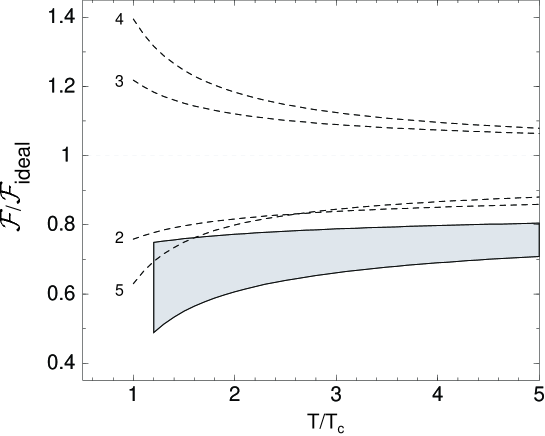
FIG. 2.: The free energy for QCD with $N_{f}=3$ quarks as a function of $T/T_{c}$. The HTL free energy is shown as a shaded band that corresponds to varying $\mu_{3}$ and $\mu_{4}$ by a factor of two around their central values. The weak-coupling expansion through orders $\alpha_{s}$, $\alpha_{s}^{3/2}$, $\alpha_{s}^{2}$, and $\alpha_{s}^{5/2}$ are shown as dashed lines labelled by 2, 3, 4 and 5.

Lattice gauge theory has been used to calculate the equation of state of a quark-gluon plasma with $N_{f}=2$ [11, 12] and $N_{f}=4$ [13] flavors of dynamical quarks. These calculations indicate that the pressure, which is the negative of the free energy, approaches that of an ideal gas from below. The approach to the ideal gas is more rapid than the leading order HTL result. For $N_{f}=4$, it reaches 80% of the value for an ideal gas already at $T=2.5\,T_{c}$. For higher values of $T$, the leading order HTL result lies significantly below the lattice results. This is not of great concern, because the difference can be accounted for by the next-to-leading order correction in HTL perturbation theory. At next-to-leading order, there are two-loop diagrams and one-loop diagrams with HTL counterterms. The contributions of order $\alpha_{s}$ coming from the hard momentum regions of the two-loop diagrams will reproduce the order-$\alpha_{s}$ term in the conventional perturbative series (46). The contribution from the HTL counterterm diagram will precisely cancel the order-$\alpha_{s}$ term in the one-loop HTL free energy. Thus the next-to-leading order correction to ${\cal F}_{\rm HTL}/{\cal F}_{\rm ideal}$ must approach $[10(24+7N_{f})/(32+21N_{f})]\alpha_{s}/\pi$ in the limit $\alpha_{s}\to 0$. This has the correct sign and roughly the right magnitude to account for the discrepancy with the lattice results.

VI Conclusions

We have completed the calculation of the free energy of a quark-gluon plasma to leading order in HTL perturbation theory by calculating the quark contribution. The quark term has a quadratic ultraviolet divergence that vanishes with dimensional regularization, but it has no logarithmic ultraviolet divergences. Comparing our result to the weak-coupling expansions for the free energy, we find that the error is of order $\alpha_{s}$ but the large correction proportional to $\alpha_{s}^{3/2}$ is included exactly. It is therefore possible that the HTL perturbative expansion for the free energy will have much better convergence properties than the conventional weak-coupling expansion. To verify this, it will be necessary to extend the calculations of the free energy to next-to-leading order in HTL perturbation theory.

A Integrals

In this appendix, we collect the results for the integrals that are required to calculate the contribution from quarks to the one-loop HTL free energy. We use dimensional regularization, so that power ultraviolet divergences are set to zero and logarithmic ultraviolet divergences appear as poles in $\epsilon$. In the HTL free energy, the ultraviolet divergences are isolated in subtraction terms that must be expanded around $\epsilon=0$ through order $\epsilon^{0}$. The integrals required to evaluate the subtractions in the quasiparticle terms are

$$\int_{0}^{\infty}dk\;k^{2-2\epsilon}\sqrt{k^{2}+m^{2}} = -{1\over 16}m^{4-2\epsilon}\left[{1\over\epsilon}+2\log 2-{1\over 2}\right]\,,$$ (A.1)

$$\int_{0}^{\infty}dk\;k^{2-2\epsilon}{1\over(k^{2}+m^{2})^{3/2}} = {1\over 2}m^{-2\epsilon}\left[{1\over\epsilon}+2\log 2-2\right]\,,$$ (A.2)

$$\int_{0}^{\infty}dk\;k^{2-2\epsilon}{1\over(k^{2}+m^{2})^{3/2}}\log{k^{2}+m^{2}\over m^{2}} = {1\over 2}m^{-2\epsilon}\left[{1\over\epsilon^{2}}-4+{\pi^{2}\over 6}-2\log^{2}2+4\log 2\right]\,.$$ (A.3)

The integrals required to evaluate the subtractions in the Landau-damping terms are

$$\int_{0}^{\infty}d\omega\;\omega\int_{\omega}^{\infty}dk\;k^{-1-2\epsilon}{1\over k^{2}-\omega^{2}+m^{2}} = {1\over 4}m^{-2\epsilon}\left[{1\over\epsilon^{2}}+{\pi^{2}\over 6}\right]\,,$$ (A.4)

$$\int_{0}^{\infty}d\omega\;\int_{\omega}^{\infty}dk\;k^{-2-2\epsilon}{k^{2}-\omega^{2}\over k^{2}-\omega^{2}+m^{2}}\log{k+\omega\over k-\omega} = m^{-2\epsilon}\left[{\log 2\over\epsilon}-2\log 2+\log^{2}2\right]\,.$$ (A.5)

REFERENCES

• [1] P. Arnold and C. Zhai, Phys. Rev. D50, 7603 (1994); Phys. Rev. D51, 1906 (1995).
• [2] B. Kastening and C. Zhai, Phys. Rev. D52, 7232 (1995).
• [3] E. Braaten and A. Nieto, Phys. Rev. Lett. 76, 1417 (1996); Phys. Rev. D53, 3421 (1996).
• [4] B. Kastening, Phys. Rev. D56, 8107 (1997); T. Hatsuda, Phys. Rev. D56, 8111 (1997).
• [5] J.P. Blaizot, E. Iancu, and A. Rebhan, Phys. Rev. Lett. 83, 2606 (1999); J.P. Blaizot, E. Iancu, and A. Rebhan, hep-ph/9910309.
• [6] J.O. Andersen, E. Braaten and M. Strickland, Phys. Rev. Lett. 83, 2139 (1999); J.O. Andersen, E. Braaten and M. Strickland, hep-ph/9905337.
• [7] E. Braaten and R.D. Pisarski, Phys. Rev. Lett. 64, 1338 (1990); Nucl. Phys. B337, 569 (1990).
• [8] V.V. Klimov, Sov. Phys. JETP 55, 199 (1982); H.A. Weldon, Phys. Rev. D26, 1394 (1982).
• [9] R.D. Pisarski, Physica A 158, 246 (1989).
• [10] J. Fingberg, U.M. Heller and F. Karsch, Nucl. Phys. B392, 493 (1993).
• [11] S. Gottlieb et al., Phys. Rev. D55, 6852 (1997).
• [12] C.W. Bernard et al., Phys. Rev. D55, 6861 (1997).
• [13] J. Engels et al., Phys. Lett. B396, 210 (1997).