Neutrino Masses and Oscillations in Models with Large Extra Dimensions

Abstract

We discuss the profile of neutrino masses and mixings in models with large extra dimensions when right handed neutrinos are present in the branes along with the usual standard model particles. In these models, string scale must be bigger than $10^{8}$ GeV to have desired properties for the neutrinos at low energies. The lightest neutrino mass is zero and there is oscillations to sterile neutrinos that are different from other models with the bulk neutrino.

I Introduction

Last year has seen an explosion of interest and activity in theories with large extra dimensions [1, 2, 3, 4, 5, 6]. It has been realized that extra dimensions almost as large as a millimeter could apparently be hidden from many extremely precise measurements that exist in particle physics. What makes such an idea exciting is the hope that the concept of hidden space dimensions can be probed by collider as well as other experiments in not too distant future. Furthermore, it brings the string scale closer to a TeV in some scenarios, making details of string physics within reach of experiments. On the theoretical side, recent developments in strongly coupled string theories have given a certain amount of credibility to such speculations in that the size of extra dimensions can be proportional to the string coupling and therefore in the context of strongly coupled strings such large dimensions are quite plausible.

This new class of theories have a sharp distinction from the conventional grand unified theories as well as old weakly coupled string models in that in the latter case, most scales other than the weak scale and the QCD scale were assumed to be in the range of $10^{13}$ to $10^{16}$ GeV. That made it easier to understand observations such as small neutrino masses and a highly stable proton etc. Now that most scales are allowed to be small in the new models, the two particularly urgent questions that need to be answered are why is the proton stable and why are neutrinos so light. It has been speculated that proton stability may be understood by conjecturing the existence of U(1) symmetries that forbid the process. On the other hand no such simple argument for understanding small neutrino masses seems to exist. The familiar seesaw mechanism[10] is not implementable in simple versions of these models where all scales are assumed to be low. So understanding lightness of neutrinos is therefore a challenge to such models.

One approach to this problem discussed in recent literature[7, 8] is to use neutrinos that live in the bulk (they are therefore necessarily singlet or sterile with respect to normal weak interactions) and to observe that their coupling to the known neutrinos in the brane is inversely proportional to the square-root of the bulk volume. The neutrino mass (which is now a Dirac mass) can be shown to be $\sim\frac{hvM^{*}}{M_{P\ell}}$, where $M^{*}$ is the string scale. If the string scale is in the TeV range, this leads to a neutrino mass of order $10^{-4}$ eV or so. This therefore explains why the neutrino masses are small. A key requirement for small neutrino masses is therefore that the string scale be in the few TeV range. Furthermore, these models also generally predict oscillations between the modes of the bulk neutrino and the known neutrinos. Thus if one wants an explanation of the solar neutrino deficit via neutrino oscillations, this implies that there must be at least one extra dimension with size in the micrometer range[8, 9]. The latter provides an interesting connection between neutrino physics, gravity experiments searching for deviations from Newton’s law at sub-millimeter distances as well as possible collider search for TeV string excitations. It then follows that larger values of the string scale would jeopardize this simple explanation of the small neutrino mass. So the extent that larger values of string scale are also equally plausible as the TeV value, one might search for alternative ways to understand the small neutrino masses.

It is the goal of this paper to outline such a scenario and study its consequences. The particular example we consider illustrates this scenario in models with large extra dimensions and generic brane-bulk picture for particles, where the string scale is necessarily bigger ($\geq 10^{8}$ GeV or so) and solar or atmospheric neutrino oscillations require at least one extra dimension be in the micrometer range. The new ingredient of the class of models we discuss here is that we include the right-handed neutrino in the brane and consider the gauge interactions to be described by a left-right symmetric model. In these models, the left-handed neutrinos are not allowed to form mass terms with the bulk neutrino due to extra gauge symmetries; instead it is only the right-handed neutrino which is allowed to form mass terms with the bulk neutrinos. This leads to a different profile for the neutrino masses and mixings. In particular, we find that in this model, the left-handed neutrino is excatly massless whereas the bulk sterile neutrinos have masses related to the size of the extra dimensions and it will be of order $\sim 10^{-3}$ eV if there is at least one large extra dimension with size in the micrometer range. A key distinguishing feature of this model from the existing ones is that the string scale is now necessarily much larger than a TeV. We also find that the pattern of the neutrino oscillations is different from the previous case.

As mentioned, the minimal gauge model where our scheme is realized is the left-right symmetric models where the right handed symmetry is broken by the doublet Higgs bosons $\chi_{R}(1,2,1)$. The notation we follow is that the three numbers inside the parenthesis correspond to the quantum numbers under $SU(2)_{L}\times SU(2)_{R}\times U(1)_{B-L}$. We do not need supersymmetry for our discussion and will therefore work within the context of nonsupersymmetric left-right models.

To set the stage for our discussion, let us start with a review of the neutrino mass mechanism in models with large extra dimensions discussed in Ref.[7]. The basic idea is to include the coupling of bulk neutrino $\nu_{B}(x^{\mu},y)$ (which is a standard model singlet) to the standard model lepton doublet $L(x^{\mu},y=0)$. The Lagrangian that is responsible for the neutrino masses in this model is:

$${\cal S}=\kappa\int d^{4}x\bar{L}H\nu_{B}(x,y=0)+\int d^{4}xdy\bar{\nu}_{B}(x,y)\Gamma^{5}\partial_{5}\nu_{B}(x,y)+h.c.$$ (1)

Writing the four component spinor $\nu_{B}\equiv\left(\begin{array}[]{c}\nu^{1}_{B}\\ i\sigma_{2}\nu^{2*}_{B}\end{array}\right)$, we get for the neutrino mass matrix:

$$(\bar{\nu}_{eL}\bar{\nu}^{\prime}_{BL})\left(\begin{array}[]{cc}\kappa v&\sqrt{2}\kappa v\\ 0&\partial_{5}\end{array}\right)\left(\begin{array}[]{c}\nu_{0B}\\ \nu^{\prime}_{BR}\end{array}\right)$$ (6)

This is a compact way of writing the KK excitations along the fifth dimension. Notice that the $\sqrt{2}$ in the off-diagonal term appears to compensate the different normalization of the zero mode in the Fourier expansion of the bulk field in terms of $\sin ny/R$ and $\cos ny/R$ ($R$ being the radius of the fifth dimension). Also, notice that only the last terms may couple to the pure four dimensional fields, and we always may choose these modes to have positive KK masses. In the above equation $\kappa$ embodies the features of the string scale and the radius of the extra dimension i.e. $\kappa\simeq\frac{M^{*}}{M_{P\ell}}$. For $\kappa v\ll\mu_{0}$ where $\mu_{0}=R^{-1}$, we get the mixing of the $\nu_{e}$ with the bulk modes to be

$$tan\theta_{eB}\approx\frac{\sqrt{2}\kappa v\partial_{5}}{\partial^{2}_{5}-\kappa^{2}v^{2}}$$ (7)

Substituting the eigenvalues of the operator $\partial_{5}=n\mu_{0}$, we get for the n-th KK excitation a mixing $tan\theta_{n}\approx\frac{\xi}{n}$ where $\xi\approx\frac{\sqrt{2}\kappa v}{\mu_{0}}$. This expression is same as in [7, 8].

Important point to note here is that since $\nu_{e}$ has a mass of $\kappa v$, present neutrino mass limits lead to an upper limit on $\kappa$ and hence on the string scale. For instance, if we choose the present tritium decay bounds[11] of $m_{\nu_{e}}\leq 2.5$ eV, we get $M^{*}\leq 10^{7}$ GeV. This bound gets considerably strengthened if we further require that the solar neutrino puzzle be solved via $\nu_{e}-\nu_{s}$ oscillation (where we have called the typical excited models of the bulk neutrino as “sterile neutrinos”). The reason is that this requires $\Delta m^{2}\simeq 10^{-5}$ eV² and in the absence of any unnatural fine tuning, we will have to assume that that $m_{\nu_{e}}\simeq m_{\nu_{s}}\simeq 10^{-3}$ eV. This implies that $M^{*}\leq 10$ TeV and the bulk radius is given by $R^{-1}\simeq 10^{-3}$ eV implying $R\simeq 0.2$ mm. Another prediction of this model is that the mixing of the $\nu_{e}$ with the bulk neutrinos goes down like $(1/n)$ where $n$ denotes the level of Kaluza-Klein excitation.

Let us now proceed to the new case we are considering. The part of the action relevant to our discussion is given by:

$${\cal S}=\int d^{4}x[\kappa\bar{L}\chi_{L}\nu_{B}(x,y=0)+\kappa\bar{R}\chi_{R}\nu_{B}(x,y=0)+h\bar{L}\phi R]+\int d^{4}xdy\bar{\nu}_{B}\Gamma^{5}\partial_{5}\nu_{B}+h.c.$$ (8)

where $L^{T}=(\nu_{eL},e_{L})$ and $R^{T}=(\nu_{eR},e_{R})$ and $\phi$ is the bidoublet Higgs field that breaks the elctroweak symmetry and gives mass to the charged fermions. We assume that the $SU(2)_{R}$ gauge group is broken by $<\chi^{0}_{R}>=v_{R}$ with $<\chi^{0}_{L}>=0$ and the $SU(2)_{L}\times U(1)_{Y}$ is broken by $Diag<\phi>=(v,v^{\prime})$. The profile of the neutrino mixing matrix in this case is given by

$$(\bar{\nu}_{eL}~{}\bar{\nu}_{0BL}~{}\bar{\nu}^{\prime}_{BL})\left(\begin{array}[]{cc}hv&0\\ \kappa v_{R}&0\\ \sqrt{2}\kappa v_{R}&\partial_{5}\end{array}\right)\left(\begin{array}[]{c}\nu_{eR}\\ \nu^{\prime}_{BR}\end{array}\right)$$ (14)

where $hv$ is the usual Dirac mass term present in the models with the seesaw mechanism and normally assumed to be of order of typical charged fermion masses (we will also make this plausible assumption that $hv$ is of the order of a few MeV’s for the first generation which will be the focus of this article).

We can now proceed to find the eigenstates and neutrino mixings. First point to note is that this matrix being $2\times 3$ has one zero eigenvalue corresponding to the state[12]

$$\nu_{0}=(\cos\zeta~{}\nu_{eL}-\sin\zeta~{}\nu_{0BL})$$ (15)

where $sin\zeta=\frac{hv}{\sqrt{(\kappa v_{R})^{2}+(hv)^{2}}}$. If we want the lightest eigenstate to be predominantly the electron neutrino so that observed universality in charged current weak interaction is maintained, we must demand that $\kappa v_{R}\gg hv$. Since $\kappa\simeq\frac{M^{*}}{M_{P\ell}}$, this constraint will imply a constraint on the string scale $M^{*}$.

Let us see under what circumstances this condition is satisfied. Since the Dirac mass $hv\simeq$ few MeV’s, we would like $\kappa v_{R}\gg$ few MeV’s. Let us assume that there is one extra dimension with large size (of order milli-meter and denoted by $R_{1}$) and all other extra dimensions have very small sizes, assumed to be equal. Then the observed strength of gravitational interaction implies the relation

$$M^{2}_{P\ell}={M^{*}}^{n+2}R^{n-1}R_{1}$$ (16)

where $R_{1}$ is the largest dimension and the rest of the R’s are small as required by neutrino physics. For simplicity let us identify the right handed symmetry breaking scale, the string scale and the inverse radii of the small dimensions $R^{-1}$. Then we have the approximate relation that

$$\kappa\simeq\frac{1}{\sqrt{M^{*n}R^{n-1}R_{1}}}\simeq\frac{M^{*}}{M_{P\ell}}$$ (17)

$\kappa v_{R}\gg$ few MeV (say 100 MeV), implies that $M^{*}\simeq v_{R}\approx R^{-1}\geq 10^{8.5}$ GeV. In fact it is not hard to see that to satisfy the relation in Eq. (16), the radii of the “small” compact dimensions must be also of order ${M^{*}}^{-1}$ and that of the large dimension is of course in the sub-millimeter range. While this is a generic possibility, one can of course make many variations on this general theme. The results of this paper are not effected by such variations. Thus it appears that our scheme prefers a high string scale in contrast with the earlier proposal[7].

We can now look at the rest of the neutrino spectrum arising from the KK excitations of the bulk mode as well as the right handed neutrino. They can be studied by looking at the “$2\times 2$” matrix after extracting the zero mode discussed above. Defining the orthogonal combination to $\nu_{0}$ as $\tilde{\nu}_{0L}$, we have:

$$(\bar{\tilde{\nu}}_{0L}~{}\bar{\nu}^{\prime}_{BL})\left(\begin{array}[]{cc}\kappa v_{R}&0\\ \sqrt{2}\kappa v_{R}&\partial_{5}\end{array}\right)\left(\begin{array}[]{c}\nu_{eR}\\ \nu^{\prime}_{BR}\end{array}\right)$$ (22)

where $\tilde{\nu}_{0L}=\cos\zeta~{}\nu_{0BL}+\sin\zeta~{}\nu_{eL}$ and we have used the approximation that $\kappa v_{R}\gg hv$. In terms of this short handed notation, the characteristic equation of the Dirac mass matrix above is easily computed to be

$$(m^{2}-\partial_{5}^{2})\left[m^{2}-\kappa^{2}v_{R}^{2}+{2m^{2}\kappa^{2}v_{R}^{2}\over\partial_{5}^{2}-m^{2}}\right]=0,$$ (23)

This, in a manner similar that noted by Dienes et al.[7] translates into the transcendental equation

$$m_{n}=\pi\kappa^{2}v_{R}^{2}R\ \cot(\pi m_{n}R)$$ (24)

where $m_{n}$ is the mass of the n-th KK state. The tower of eigenstates, symbolically denoted by $\nu_{nL}$, are exactly given by

$$\nu_{nL}={1\over\eta_{n}}\left[{\tilde{\nu}}_{0L}+{\sqrt{2}m_{n}^{2}\over m^{2}-\partial_{5}^{2}}~{}\nu^{\prime}_{BL}\right],$$ (25)

with the normalization factor, $\eta_{n}$, given as

$$\eta_{n}^{2}=1+\sum_{k=1}^{\infty}{2m_{n}^{4}R^{4}\over(k^{2}-m_{n}^{2}R^{2})^{2}}.$$ (26)

As long as $\kappa v_{R}R\gg 1$, all the mass eigenvalues, $m_{n}$ upto $m_{n}\sim\kappa v_{R}$ satisfy $cot(\pi m_{n}R)\approx 0$. Therefore, the masses for all these states are $\sim(2n-1)/2R$. Thus the effect of the mixing of the brane righthanded neutrinos is to shift the bulk neutrino levels below and near $\kappa v_{R}$ downward. This is similar to what was noted in the case without the $\nu_{R}$ in the brane[7] for all states. On the other hand, using the same equation (Eq. (11)) it is easy to see that the states much heavier than $\kappa v_{R}$ have masses $\sim n/R$, which also means that they basically decouple from the light sector. For the eigenstates in the middle, those with masses just beyond $\kappa v_{R}$, their mixing with the lightest states strongly suppress their contribution to $\tilde{\nu}_{0L}$, by an amount $\sim 1/\kappa v_{R}R$, as it could be checked from Eq. (26), by summing over those elements for which $k\ll\kappa v_{R}R$.

There are, of course, similar results for the right handed states which involve the right handed bulk neutrinos. In fact, they are identified as the negative solutions to the characteristic equation, since the same mass matrix gives the masses of both left and right handed sectors and those are degenerate.

For discussing neutrino oscillation, the left handed eigenstates are the only ones relevant. For this purpose let us write down the weak eigenstate $\nu_{e}$ in terms of the mass eigenstates through their mixing into $\tilde{\nu}_{0}$. Since $\nu_{e}=c_{\zeta}~{}\nu_{0}+s_{\zeta}~{}\tilde{\nu}_{0}$, with $c_{\zeta}$ ($s_{\zeta}$) standing for $\cos\zeta$ ($\sin\zeta$), the survival probability of $\nu_{e}$ oscillations reads

$$P(\nu_{e}\rightarrow\nu_{e}(t))=c_{\zeta}^{4}+s_{\zeta}^{4}~{}P(\tilde{\nu}_{0}\rightarrow\tilde{\nu}_{0}(t))+2~{}c_{\zeta}^{2}~{}s_{\zeta}^{2}~{}Re\langle\tilde{\nu}_{0}|\tilde{\nu}_{0}(t)\rangle,$$ (27)

where $P(\tilde{\nu}_{0}\rightarrow\tilde{\nu}_{0}(t))$ is the corresponding “survival probability” for $\tilde{\nu}_{0}$. In terms of the mass eigenstates

$$\tilde{\nu}_{0}(t)=\sum_{n=1}^{N}{e^{i(m_{n}^{2}t/2E)}\over\eta_{n}}\nu_{n},$$ (28)

where we have cut off the sum by $N\approx\kappa v_{R}R$, explicitly decoupling the heavy eigenstates. This is justified by the arguments given above. For the remaining states, one can show that $\eta_{n}^{2}\approx{\pi^{2}\over 8}(2n-1)^{2}$ which follows from the following exact expression for $\eta^{2}_{n}$:

$$\eta^{2}_{n}~{}=~{}1+{1\over 4}\csc^{2}(2\pi m_{n}R)\left[2\pi^{2}m^{2}_{n}R^{2}+\pi sin(2\pi m_{n}R)+2cos(2\pi m_{n}R)-2\right]$$ (29)

It means that the main contribution to $\tilde{\nu}_{0}$ comes from the lightest mode, which is expected since the bulk zero mode is its main original component. The final survival probability after the neutrino traverses a distance L in vacuum can be written down as

$$P_{ee}(E)=1-4\ c^{2}_{\zeta}\ s^{2}_{\zeta}\sum_{n=1}^{N}{1\over\eta_{n}^{2}}\sin^{2}\left({m_{n}^{2}L\over 4E}\right)-4\ s^{4}_{\zeta}\ \sum_{k<n}^{N}{1\over\eta_{n}^{2}\eta_{k}^{2}}\sin^{2}\left[{(m_{n}^{2}-m_{k}^{2})L\over 4E}\right].$$ (30)

Therefore, the oscillation length is given by $L_{osc}=ER^{2}_{1}\sim(E/MeV)\times 5\cdot 10^{4}$m for $R_{1}=0.1~{}mm$. This value for the oscillation length is right in the domain of accessibility of the KAMLAND experiment[13]. In Fig. 1 we present the survival probability as a function of distance for specific values of $\kappa v_{R}$ and $hv$. Also, we present the probability for the early proposal of Ref. [8] in Fig. 2 for comparision. Notice that the differences in both profiles come, basically, from two facts: first, the masses of the light bulk modes have been shifted down by ${1\over 2}\mu_{0}$ in the present case. Such an effect is absent in the approach followed in the former case[7]. This is reflected in a (four times) larger oscillation length. Secondly, the mixing of $\nu_{e}$ with bulk states is different in our case than Ref.[7, 8] though for large values of $n$ they coincide.

The averaged probability is now obtained in a stgraightforward manner to be $\overline{P_{ee}}=c_{\zeta}^{4}+{2\over 3}s_{\zeta}^{4}$, which is smaller than the two neutrino case with the same mixing angle, although, for $\zeta\ll 1$ it approaches the former result $\overline{P_{ee}}\approx 1-2\zeta^{2}$. Moreover, we may average over all the modes, but the lowest frequency one, to get

$$P_{ee}(E)=c_{\zeta}^{4}+{2\over 3}s_{\zeta}^{4}+{16\over\pi^{2}}c_{\zeta}^{2}\ s_{\zeta}^{2}\ \left[1-2\sin^{2}\left({\mu_{0}^{2}L\over 16E}\right)\right].$$ (31)

Hence, the depth of the oscillations is now of the order of ${32\over\pi^{2}}c_{\zeta}^{2}s_{\zeta}^{2}$.

In conclusion, we have presented a new way to understand small neutrino masses in models with large extra dimensions by including the righthanded neutrino among the brane particles. In addition to several quantitative differences from earlier works which have only then standard model particles in the brane, we find that the string scale in the new class of models is necessarily larger. However, we need one extra dimension to be of large size if we want to solve the solar neutrino problem as well have other meaningful oscillations between the known neutrinos with the bulk neutrinos.

We have not discussed the matter effect and the implications for solar neutrino puzzle nor have we discussed the astrophysical constraints on our scenario. We hope to return to these topics subsequently. But we have noted that multiple ripple effect induced by the KK modes in the $\nu_{e}$ survival probability that was noted for the earlier case in Ref.[8] remains in our case too.

Secondly, we have focussed only on the first generation neutrinos; but there is no obstacle in principle to extending the discussion to the other generations. Clearly, as in the case of Ref.[8], attempting to solve the atmospheric neutrino puzzle by $\nu_{\mu}$-$\nu_{bulk}$ oscillation would require that we make the bulk radius $R_{1}$ smaller.

Our overall impression is that while it is possible to understand the smallness of the neutrino mass using the bulk neutrinos without invoking the seesaw mechanism and concommitant high scale physics such as $B-L$ symmetry, a unified picture that clearly incorporates all three generations with preferred mixing and mass patterns[14] is yet to come whereas in existing “four-dimensional” models there exist perhaps a surplus of ideas that lead to desirable neutrino mass textures. ¿From this point of view, the neutrino physics study in models with extra diensions is still in its infancy and whether it grows into adulthood depends much on the direction that these extra dimensional models take in the coming years.

Acknowledgements. The work of RNM is supported by a grant from the National Science Foundation under grant number PHY-9802551. The work of SN is supported by the DOE grant DE-FG03-98ER41076. The work of APL is supported in part by CONACyT (México). RNM would like to thank the Institute for Nuclear Theory at the University of Washington for hospitality and support during the last stages of this work. SN gratefully acknowledges the warm hospitality and support during his visit to the University of Maryland particle theory group when this work was started and to the Fermilab theory group where it was completed.

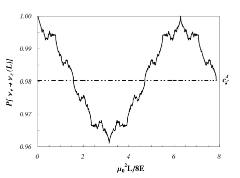
FIG. 1.: Profile of the survival probability for $\nu_{e}$ oscillations obtained for $\kappa v_{R}=100$ MeV and $hv=10$ MeV. The horizontal line corresponds to the value of $\cos^{4}\zeta$

FIG. 2.: Profile of the survival probability for $\nu_{e}$ oscillations for the model of first Ref. in [8] using $\xi=0.1$. Notice that the argument is augmented by a factor of four with respect to the case in the previous figure.

REFERENCES

- [1] I. Antoniadis, Phys. Lett. B246 (1990) 377; I. Antoniadis, K. Benakli and M. Quirós, Phys. Lett. B331 (1994) 313.
- [2] E. Witten, Nucl. Phys. B 471, 135 (1996); P. Horava and E. Witten, Nucl. Phys. B475 (1996) 94.
- [3] J. Lykken, Phys. Rev. D54 (1996) 3693.
- [4] N. Arkani-Hamed, S. Dimopoulos and G. Dvali, Phys. Lett. B429 (1998) 263; Phys. Rev. D59 (1999) 086004; I. Antoniadis, S. Dimopoulos, G. Dvali, Nucl. Phys. B516 (1998) 70.
- [5] K.R. Dienes, E. Dudas and T. Gherghetta, Phys. Lett. B436 (1998) 55; Nucl. Phys. B537 (1999) 47.
- [6] K. Benakli, hep-ph/9809582,Phys. Lett. B447 (1999) 51; P.Nath and M. Yamaguchi, hep-ph/9903298; hep-ph/9902323; M. L. Graesser, hep-ph/9902310; M. Masip and A. Pomarol, hep-ph/9902467; T. Banks, A. Nelson and M. Dine, JHEP 9906 (1999) 014; D. Ghilencea and G.G. Ross, Phys. Lett. B442 (1998) 165; Z. Kakushadze, Nucl. Phys. B548 (1999) 205; C.D. Carone, Phys. Lett. B454 (1999) 70; A. Delgado and M. Quirós, hep-ph/9903400. P. H. Frampton and A. Rǎsin, hep-ph/9903479; G. Giudice, R. Rattazzi and J. Wells, Nucl. Phys. B544 (1999) 3; E. Mirabelli, M. Perelstein and M. Peskin, Phys. Rev. Lett.82 (1999) 2236; T. Han, J. Lykken and R. J. Zhang, Phys. Rev. D59 (1999) 105006; J. L. Hewett, Phys. Rev. Lett.82 (1999) 47656; P. Mathews, S. Raychaudhuri and K. Sridhar, Phys. Lett. B450 (1999) 343; T. G. Rizzo, Phys. Rev. D59 (1999) 115010; K. Aghase and N. G. Deshpande, Phys. Lett. B456 (1999) 60; K. Cheung and W. Y. Keung, hep-ph/9903294; T. Taylor and G. Veneziano, Phys. Lett. B212 (1988) 147; C. Burgess, L. Ibañez and F. Quevedo, Phys. Lett. B447 (1999) 257; A. P. Lorenzana and R. N. Mohapatra, hep-ph/9904504; K. Huitu and T. Kobayashi, hep-ph/9906431. D. Dumitru and S. Nandi, hep-ph/9906514; C. Balazs, H. -J He, W. W. Repko, C. P. Yuan and D. A. Dicus, hep-ph/9904220; T. Han, D. Rainwater and D. Zepenfield, hep-ph/9905423; W. J. Marciano, hep-ph/9903451; A. Delgardo and M. Quiros, hep-ph/9903400; H. C. Cheng, B. Dobrescu and C. Hill, hep-ph/9906327; T. Rizzo and J. Wells, hep-ph/9906234.
- [7] K.R. Dienes, E. Dudas and T. Gherghetta, hep-ph/9811428; N. Arkani-Hamed, S. Dimopoulos, G. Dvali and J. March-Russell, hep-ph/9811448.
- [8] G. Dvali and A.Yu. Smirnov, hep-ph/9904211.
- [9] A. Faraggi and M. Pospelov, hep-ph/9901299; A. Das and O. C. W. Kong, hep-ph/9907272.
- [10] M. Gell-Mann, P. Ramond and R. Slansky, in Supergravity, eds. P. van Niewenhuizen and D.Z. Freedman (North Holland 1979); T. Yanagida, in Proceedings of Workshop on Unified Theory and Baryon number in the Universe, eds. O. Sawada and A. Sugamoto (KEK 1979); R. N. Mohapatra and G. Senjanović, Phys. Rev. Lett. 44, 912 (1980).
- [11] C. Weinheimer, Invited talk at the workshop on Lepton Moments, Heidelberg, June (1999); V. Lobashev et al. Phys. Lett B (to appear).
- [12] L. Wolfenstein and D. Wyler, Nucl. Phys. B 218, 205 (1983).
- [13] F. Suekane et al. preprint TOHOKU-HEP-97-02 (1997).
- [14] For recent reviews see, S. Bilenky, C. Giunti and W. Grimus, hep-ph/9812360, to appear in Prog. in Particle and Nucl. Phys., vol. 43; B. Kayser, P. Fisher and K. Macfarland, hep-ph/9906244 (to appear in the Ann. Rev. of Nucl. and Part. Sc., 1999).