LBNL-43048

BNL-HET-99/10

ATL-COM-PHYS-99-018

Measurements in SUGRA Models
with Large $\tan\beta$ at LHC

I. Hinchliffe^a and F.E. Paige^b

^aLawrence Berkeley National Laboratory, Berkeley, CA

^bBrookhaven National Laboratory, Upton, NY

We present an example of a scenario of particle production and decay in supersymmetry models in which the supersymmetry breaking is transmitted to the observable world via gravitational interactions. The case is chosen so that there is a large production of tau leptons in the final state. It is characteristic of large $\tan\beta$ in that decays into muons and electrons may be suppressed. It is shown that hadronic tau decays can be used to reconstruct final states.

1 Introduction

If supersymmetry (SUSY) exists at the electroweak scale, then gluinos and squarks will be copiously produced in pairs at the LHC and will decay via cascades involving other SUSY particles. The characteristics of these decays and hence of the signals that will be observed and the measurements that will be made depend upon the actual SUSY model and in particular on the pattern of supersymmetry breaking. Previous, detailed studies of signals for SUSY at the LHC [1, 2, 3, 4] have used the SUGRA model [5, 6], in which the supersymmetry breaking is transmitted to the sector of the theory containing the Standard Model particles and their superpartners via gravitational interactions. The minimal version of this model has just four parameters plus a sign. The lightest supersymmetric particle (${\tilde{\chi}_{1}^{0}}$) has a mass of order 100 GeV, is stable, is produced in the decay of every other supersymmetric particle and is neutral and therefore escapes the detector. The strong production cross sections and the characteristic signals of events with multiple jets plus missing energy $\hbox to0.0pt{\hbox to7.95831pt{\hfil/\hfil}\hss}E_{T}$ or with like-sign dileptons $\ell^{\pm}\ell^{\pm}$ plus $\hbox to0.0pt{\hbox to7.95831pt{\hfil/\hfil}\hss}E_{T}$ [7] enable SUSY to be extracted trivially from Standard Model backgrounds. Characteristic signals were identified that can be exploited to determine, with great precision, the fundamental parameters of these model over the whole of its parameter space. Variants of this model where R-Parity is broken [8] and the ${\tilde{\chi}_{1}^{0}}$ is unstable have also been discussed [9].

These models have characteristic final states depending upon their parameters. The next to lightest neutral gaugino $\tilde{\chi}_{2}^{0}$ is produced in the decays of squarks and gluinos which themselves may be produced copiously at the LHC. The decay of $\tilde{\chi}_{2}^{0}$ then provides a tag from which the detailed analysis of supersymmetric events can begin. The dominant decay is usually either $\tilde{\chi}_{2}^{0}\to h{\tilde{\chi}_{1}^{0}}$ or $\tilde{\chi}_{2}^{0}\to\ell^{+}\ell^{-}{\tilde{\chi}_{1}^{0}}$, which can proceed directly or via the two step decay $\tilde{\chi}_{2}^{0}\to\ell^{+}\tilde{\ell^{-}}\to\ell^{+}\ell^{-}{\tilde{\chi}_{1}^{0}}$. The latter leads to events with isolated leptons. Both of these characteristic features have been explored in some detail in previous studies [2, 3, 4].

In the previous cases the smuon, selectron and stau were essentially degenerate. At larger values of $\tan\beta$, this degeneracy is lifted and the ${\tilde{\tau}}_{1}$ becomes the lightest slepton. If $m_{1/2}$ is small enough, then the two-body decays $\tilde{\chi}_{2}^{0}\to{\tilde{\chi}_{1}^{0}}h$, ${\tilde{\chi}_{1}^{0}}Z$ will not be allowed, and if $m_{0}$ is large enough, then $\tilde{\chi}_{2}^{0}\to{\tilde{\ell}}_{R}\ell$ will also not be allowed. Then for large enough $\tan\beta$ the only allowed two-body decays are $\tilde{\chi}_{2}^{0}\to\tau^{\pm}\tilde{\tau}^{\mp}\to\tau^{+}\tau^{-}{\tilde{\chi}_{1}^{0}}$. In such cases, tau decays are dominant, and final states involving tau’s must be used.

The simulation in this paper is based on the implementation of the minimal SUGRA model in ISAJET [10]. We use $m_{0}=m_{1/2}=200$ GeV, $\tan\beta=45$, $A_{0}=0$ and $\mathop{\rm sgn}\mu=-1$. The mass spectrum for this case is shown in Table 1. The only allowed two-body decay of $\tilde{\chi}_{2}^{0}$ is into ${\tilde{\tau}}_{1}\tau$, so it has a branching ratio of more than 99%.

Table 1: Masses of the superpartners, in GeV, for the case being studied. Note that the first and second generation squarks and sleptons are degenerate and so are not listed separately.

Sparticle	mass	Sparticle	mass
$\widetilde{g}$	540
$\widetilde{\chi}_{1}^{\pm}$	151	$\widetilde{\chi}_{2}^{\pm}$	305
$\widetilde{\chi}_{1}^{0}$	81	$\widetilde{\chi}_{2}^{0}$	152
$\widetilde{\chi}_{3}^{0}$	285	$\widetilde{\chi}_{4}^{0}$	303
$\widetilde{u}_{L}$	511	$\widetilde{u}_{R}$	498
$\widetilde{d}_{L}$	517	$\widetilde{d}_{R}$	498
$\widetilde{t}_{1}$	366	$\widetilde{t}_{2}$	518
$\widetilde{b}_{1}$	391	$\widetilde{b}_{2}$	480
$\widetilde{e}_{L}$	250	$\widetilde{e}_{R}$	219
$\widetilde{\nu}_{e}$	237	$\widetilde{\tau}_{2}$	258
$\widetilde{\tau}_{1}$	132	$\widetilde{\nu}_{\tau}$	217
$h^{0}$	112	$H^{0}$	157
$A^{0}$	157	$H^{\pm}$	182

The total production cross-section for this model is 99 pb at the LHC. The rates are dominated by the production of $\tilde{g}\tilde{g}$ and $\tilde{g}\tilde{q}$ final states. Interesting decays include:

• $BR(\tilde{\chi}_{2}^{0}\to\tau\tilde{\tau_{1}})=99.9$%; $BR(\tilde{\chi}_{1}^{+}\to\nu_{\tau}\tilde{\tau_{1}})=99.9$%

• $BR(\tilde{\chi}_{3}\to\tilde{\chi}_{2}^{0}Z)=$13%; $BR(\tilde{\chi}_{3}\to\tau\tilde{\tau_{1}})=21$%;

• $BR(\tilde{g}\to b\tilde{b_{1}})=55$%; $BR(\tilde{g}\to b\tilde{b_{2}})=10$%;

• $BR(\tilde{g}\to q_{R}\tilde{q_{l}})=3$%; $BR(\tilde{g}\to q_{r}\tilde{q_{r}})=5.7$%;

• $BR(\tilde{q_{L}}\to\tilde{\chi}_{2}^{0}q)=30$%; $BR(\tilde{q_{R}}\to\tilde{\chi}_{1}^{0}q)=97$%;

Here $q$ refers to a light quark.

All the analyses presented here are based on ISAJET 7.37 [10] and a simple detector simulation. 600K signal events were generated which would correspond to 6 fb^-1 of integrated luminosity. The Standard Model background samples contained 250K events for each of $t\bar{t}$, $WZ$ with $W\to e\nu,\mu\nu,\tau\nu$, and $Zj$ with $Z\to\nu\bar{\nu},\tau\tau$, and 5000K QCD jets (including $g$, $u$, $d$, $s$, $c$, and $b$) divided among five bins covering $50<P_{T}<2400\,{\rm GeV}$. Fluctuations on the histograms reflect the generated statistics. On many of the plots that we show, very few Standard Model background events survive the cuts and the corresponding fluctuations are large, but in all cases we can be confident that the signal is much larger than the residual background. The cuts that we chosen have not been optimized, but rather have been chosen to get background free samples.

The detector response is parameterized by Gaussian resolutions characteristic of the ATLAS [11] detector without any tails. All energy and momenta are measured in GeV. In the central region of rapidity we take separate resolutions for the electromagnetic (EMCAL) and hadronic (HCAL) calorimeters, while the forward region uses a common resolution:

$${\rm EMCAL} \phantom{0}10\%/\sqrt{E}\oplus 1\%,\quad|\eta|\,<3\,$$

$${\rm HCAL} \phantom{0}50\%/\sqrt{E}\oplus 3\%,\quad|\eta|\,<3\,$$

$${\rm FCAL} 100\%/\sqrt{E}\oplus 7\%,\quad|\eta|\,>3\,$$

A uniform segmentation $\Delta\eta=\Delta\phi=0.1$ is used with no transverse shower spreading. Both ATLAS [11] and CMS [12] have finer segmentation over most of the rapidity range, but the neglect of shower spreading is unrealistic, especially for the forward calorimeter. Missing transverse energy is calculated by taking the magnitude of the vector sum of the transverse energy deposited in in the calorimeter cells. An oversimplified parameterization of the muon momentum resolution of the ATLAS detector — including a both the inner tracker and the muon system measurements — is used, viz

$$\delta P_{T}/P_{T}=\sqrt{0.016^{2}+(0.0011P_{T})^{2}}$$

For electrons we use a momentum resolution obtained by combining the electromagnetic calorimeter resolution above with a tracking resolution of the form

$$\delta P_{T}/P_{T}=\left(1+{0.4\over(3-\left|\eta\right|)^{3}}\right)\sqrt{(0.0004P_{T})^{2}+0.0001}$$

This provides a slight improvement over the calorimeter alone.

Jets are found using GETJET [10] with a simple fixed-cone algorithm. The jet multiplicity in SUSY events is rather large, so we will use a cone size of

$$R=\sqrt{(\Delta\eta)^{2}+(\Delta\phi)^{2}}=0.4$$

unless otherwise stated. Jets are required to have at least $P_{T}>20\,{\rm GeV}$; more stringent cuts are often used. All leptons are required to be isolated and have some minimum $P_{T}$ and $\left|\eta\right|<2.5$, consistent with the coverage of the central tracker and muon system. An isolation requirement that no more than 10 GeV of additional $E_{T}$ be present in a cone of radius $R=0.2$ around the lepton is used to reject leptons from $b$-jets and $c$-jets. In addition to these kinematic cuts a lepton ($e$ or $\mu$) efficiency of 90% and a $b$-tagging efficiency of 60% is assumed [11].

As $\tau$’s are a crucial part of this analysis, they require special treatment. We concentrate on hadronic tau decays, since for leptonic decays the origin of the lepton is not clear and the visible lepton in general carries only a small fraction of the true tau momentum. Using the fast simulation, we first identify the hadronic taus by searching the reconstructed jet list for jets with $P_{T}>20$ GeV and $\left|\eta\right|<2.5$. We then compare these jets with the generated tau momenta and assign them to a reconstructed tau if $E_{\tau}>0.8E_{jet}$ and the center of the jet and the tau are separated by $\Delta R<0.4$.

We then rely on a full simulation [13] of $Z+{\rm jet}$ events with $Z\to\tau\tau$. Events were generated with PYTHIA  [14] and passed through the ATLAS GEANT simulation (DICE) and reconstruction (ATRECON) programs  [15]. The charged particles were reconstructed with the tracking and the photons with the calorimeter. Cuts were then applied to the invariant mass and isolation of the reconstructed taus. These cuts produce a rejection factor against QCD jets of a factor of 15 and accept 41% of the hadronic tau decays. We apply these results to the hadronic tau’s identified in our fast simulation on a probabilistic basis. The accepted hadronic decays are assumed to be measured using the resolution from the full simulation, while the ones not accepted are put back into the jet list. Fake $\tau$’s are made by reassigning jets with the appropriate probability. The full simulation also indicates that the tau charge is correctly identified 92% of the time. We include this factor in our fast $\tau$ reconstruction and assign the fake tau’s to either sign with equal probability. For cases where the $\tau\tau$ invariant mass is to be measured, the generated $\tau\tau$ invariant mass is smeared with a resolution derived from the full simulation, i.e., a Gaussian with a peak at $M=0.66M_{\tau\tau}$ and $\sigma/M=0.12$. In cases where the measured momentum of the $\tau$ decay products is needed, the measured jet energy is used.

Results are presented for an integrated luminosity of $10\,{\rm fb}^{-1}$, corresponding to one year of running at $10^{33}\,{\rm cm^{-2}s^{-1}}$; pile up has not been included. We will occasionally comment on the cases where the full design luminosity of the LHC, i.e. $10^{34}\,{\rm cm^{-2}s^{-1}}$, will be needed to complete the studies. For many of the histograms shown, a single event can give rise to more than one entry due to different possible combinations. When this occurs, all combinations are included.

The rest of this paper is organized as follows. We first illustrate how measurement of the $\tau\tau$ final state can be used to infer information on the masses of the staus. We then use this final state in conjunction with $b$-jets to reconstruct gluinos and bottom squarks. Methods for extracting information on light squarks are then shown and the dilepton mass distribution is used to give information on the masses $\tilde{\chi}_{4}^{0}$. Finally we show how this information can be combined to constrain the underlying model parameters.

2 Effective mass distribution

The first step in the search for new physics is to discover a deviation from the Standard Model and to estimate the mass scale associated with it. SUSY production at the LHC is dominated by gluinos and squarks, which decay into multiple jets plus missing energy. A variable which is sensitive to inclusive gluino and squark decays is the effective mass $M_{\rm eff}$, defined as the scalar sum of the $P_{T}$’s of the four hardest jets and the missing transverse energy $\hbox to0.0pt{\hbox to7.95831pt{\hfil/\hfil}\hss}E_{T}$,

$$M_{\rm eff}=p_{T,1}+p_{T,2}+p_{T,3}+p_{T,4}+\hbox to0.0pt{\hbox to7.95831pt{\hfil/\hfil}\hss}E_{T}\,.$$

Here the jet $P_{T}$’s have been ordered such that $p_{T,1}$ is the transverse momentum of the leading jet. The Standard Model backgrounds tend to have smaller $\hbox to0.0pt{\hbox to7.95831pt{\hfil/\hfil}\hss}E_{T}$, fewer jets and a lower jet multiplicity. In addition, since a major source of $\hbox to0.0pt{\hbox to7.95831pt{\hfil/\hfil}\hss}E_{T}$ is weak decays, large $\hbox to0.0pt{\hbox to7.95831pt{\hfil/\hfil}\hss}E_{T}$ events in the Standard Model tend to have the missing energy associated with leptons. To suppress these backgrounds, the following cuts were made:

• $\hbox to0.0pt{\hbox to7.95831pt{\hfil/\hfil}\hss}E_{T}>100\,{\rm GeV}$;

• $\geq 4$ jets with $P_{T}>50\,{\rm GeV}$ and $p_{T,1}>100\,{\rm GeV}$;

• Transverse sphericity $S_{T}>0.2$;

• No $\mu$ or isolated $e$ with $P_{T}>20\,{\rm GeV}$ and $|\eta|<2.5$;

• $\hbox to0.0pt{\hbox to7.95831pt{\hfil/\hfil}\hss}E_{T}>0.2M_{\rm eff}$.

Note that some of these jets could result from hadronic tau decays. With these cuts and the idealized detector assumed here, the signal is much larger than the Standard Model backgrounds for large $M_{\rm eff}$, as is illustrated in Figure 1. Thus, the discovery strategy developed for low $\tan\beta$ [1] also works for this case. As demonstrated in more detail elsewhere [1] the shape of this effective mass distribution can be used to estimate the masses of the SUSY particles that are most copiously produced; here quarks and gluinos.

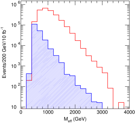
Figure 1: SUSY signal (open histogram) and Standard Model backgrounds (filled histogram).

3 Tau-Tau invariant mass

As can be seen from the decays listed above we expect significant prodution of $\tilde{\chi}_{2}^{0}$ and hence of tau pairs from the decay of $\tilde{q_{L}}$ We require that the events contain at least two jets that are indentified as hadronic tau decays using the above algorithm. In addition, the following cuts are applied:

• $\hbox to0.0pt{\hbox to7.95831pt{\hfil/\hfil}\hss}E_{T}>100\,{\rm GeV}$;

• at least four jets with $P_{T}>50\,{\rm GeV}$ and at least one jet $p_{T,1}>100\,{\rm GeV}$;

• $M_{\rm eff}>500\,{\rm GeV}$;

• $\hbox to0.0pt{\hbox to7.95831pt{\hfil/\hfil}\hss}E_{T}>0.2M_{\rm eff}$.

Again, some of these jets could result from hadronic tau decays.

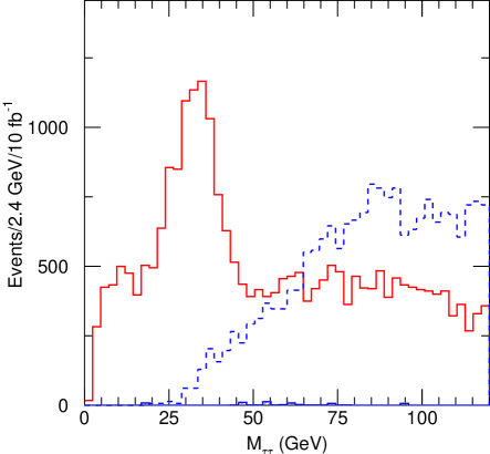
Figure 2: Reconstructed $\tau\tau$ mass distribution. All combinations of tau pairs are shown irrespective of the charge. The dashed histogram shows the comibination of one real tau and one fake tau. The actual experiement would observe the sum of the two histograms. The background from Standard Model processes is very small and is not shown.

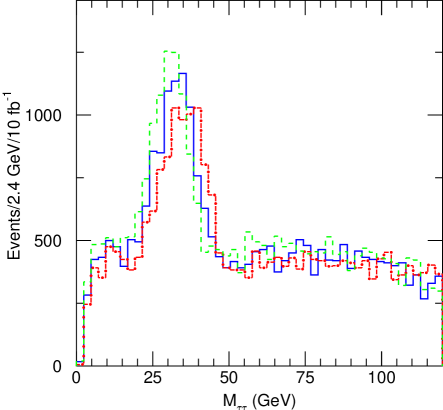
Figure 3: Reconstructed $\tau\tau$ mass distribution showing the effect of rescaling the generated tau-tau invarient mass distribution by $\pm 7.5$%.

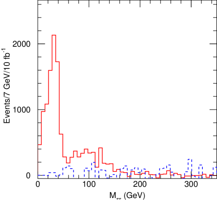
Figure 4: Reconstructed $\tau^{+}\tau^{-}-\tau^{\pm}\tau^{\pm}$ mass distribution. The dashed line shows the fake-real background. The flucuations are slightly larger than the true statistics.

We then search for taus that decay hadronically using the algrotihm discussed above. The reconstructed $\tau\tau$ invarient mass distribution is shown in Figure 2; all combinations of tau charges are shown in this Figure. It can be seen from this distribution that there is a clear structure. There is considerable background from combinations where one of the identified tau jets is from a tau and the other is from a misidentified jet. The invarient mass distribution of these pairs is also shown in Figure 2; it is rather featureless. The tau algorthm has not been optimized so this background could well have been overestimated. The background from events where both taus are misidentified jets and the Standard Model background are both negligible. The position of the peak in this mass distribution enables one to infer the position of the end point arising from the decay chain $\tilde{\chi}_{2}^{0}\to\tau\tilde{\tau}_{1}\to\tilde{\chi}_{1}^{0}\tau\tau$:

$$M_{\tau\tau}^{\rm max}=M_{\tilde{\chi}_{2}^{0}}\sqrt{1-{M_{\tilde{\ell}}^{2}\over M_{\tilde{\chi}_{2}^{0}}^{2}}}\sqrt{1-{M_{{\tilde{\chi}_{1}^{0}}}^{2}\over M_{\tilde{\ell}}^{2}}}=59.6\,{\rm GeV}.$$

In order to estimate the precision with which this endpoint can be determined, the generated tau-tau invarient mass distribution was shifted by $\pm 7.5$% from its nominal value. The effect on the reconstructed $\tau\tau$ mass distribution is shown in Figure 3. These cases can clearly be distinguished. The actual precision that can be obtained on the position of this end point requires a more detailed study. Tau decays are well understood; the problem is to determine the effects of the detector resolutions and the cuts. For the purposes of extracting parameters below, we will assume an uncertainty of 5% can be achieved.

There are some events beyond this edge as can be seen by looking at the subtracted distribution $\tau^{+}\tau^{-}-\tau^{-}\tau^{-}-\tau^{+}\tau^{+}$ shown in Figure 4. This subtraction also elliminates the background from fake taus because their charges are not correlated. Here the excess extends to $\sim 150$ GeV and is due to $\chi_{3}$ and $\chi_{4}$ decays. This can be confirmed by the large $Z$ signal (see below). The fluctuations in this histogram reflect the generated statistics, which correspond to about $6\,{\rm fb}^{-1}$; three years at low luminosity would make this high-mass signal much clearer.

4 Reconstruction of $\tilde{g}\to b\tilde{b}\to b\tilde{\chi}_{2}^{0}b\to bb\tau^{+}\tau^{-}{\tilde{\chi}_{1}^{0}}$

The event sample of the previous section is used in an attempt to reconstruct squarks and gluinos. We concentrate here on final states with $b$ quarks as these have the larger branching ratios and less combinatorial background. In addition to the previous cuts, we require a tagged $b$-jet with $P_{T}>25$ GeV; this jet could be one of the ones in the previous selection. Events are selected that have reconstructed tau pairs with invariant mass within $\pm 10$ GeV of peak in Figure 2, and the invariant mass of the tau pair and the $b$-jet is formed. This mass distribution is shown in Figure 5. The sign subtracted distribution corresponding to $\tau^{+}\tau^{-}-\tau^{-}\tau^{-}-\tau^{+}\tau^{+}$ is used to reduce combinatorial background. There should should be an edge at $\sim m_{\tilde{b}_{1}}-m_{\tilde{\chi}_{1}}=310$ GeV. The edge is not sharp — 3 particles are lost, two $\nu_{\tau}$’s and the ${\tilde{\chi}_{1}^{0}}$. In addition the distribution is contaminated by decays from $\tilde{\chi}_{3}^{0}$ and $\tilde{\chi}_{4}^{0}$. The structure is not clear, but is well distinguished from that resulting from the case where the $b$-jet is replaced by a light quark jet, shown in Figure 9.

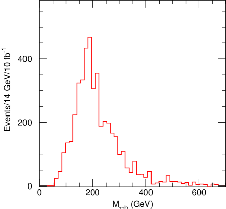
Figure 5: Reconstructed $\tau\tau+{\rm jet}$ mass distribution where the jet is tagged as a $b$-jet. The background from Standard Model processes is negligible.

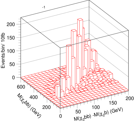
Figure 6: Lego plot showing the reconstructed masses $m(\tilde{\chi}_{2}^{0}b)$ and $m(\tilde{\chi}_{2}^{0}bb)-m(\tilde{\chi}_{2}^{0}b)$.

Further information can be obtained by applying a partial reconstruction technique. This was developed in Ref.  (so called “Point 3”) where the decay chain $\tilde{g}\to b\tilde{b}\to bb\tilde{\chi}_{2}^{0}b\to bb\ell^{+}\ell^{-}{\tilde{\chi}_{1}^{0}}$ was fully reconstructed as follows. If the mass of the lepton pair is near its maximum value, then in the rest frame of $\tilde{\chi}_{2}^{0}$ both $\tilde{\chi}_{1}$ and the $\ell^{+}\ell^{-}$ pair are forced to be at rest. The momentum of $\tilde{\chi}_{2}^{0}$ in the laboratory frame is then determined

$$\vec{P}_{\tilde{\chi}_{2}^{0}}=\left(1+M_{{\tilde{\chi}_{1}^{0}}}/M_{\ell^{+}\ell^{-}}\right)\vec{P}_{\ell^{+}\ell^{-}}\,.$$

where $P_{\ell^{+}\ell^{-}}$ is the momentum of the dilepton system. The $\tilde{\chi}_{2}^{0}$ can then be combined with b jets to reconstruct the decay chain. A clear correlation between the masses of the $b\tilde{\chi}_{2}^{0}$ and $bb\tilde{\chi}_{2}^{0}$ systems was observed allowing both the gluino and sbottom masses to be determined if the mass of ${\tilde{\chi}_{1}^{0}}$ was assumed. The inferred mass difference $m_{\tilde{g}}-m_{\tilde{b}}$ was found to be insensitive to assumed ${\tilde{\chi}_{1}^{0}}$ mass.

In the case of interest here the situation is more complicated. First, there is an extra step in the decay chain i.e.  $\tilde{g}\to b\tilde{b}\to bb\tilde{\chi}_{2}^{0}b\to bb\tau{\tilde{\tau}}\to bb\tau^{+}\tau^{-}{\tilde{\chi}_{1}^{0}}$. So that even if the events could be selected such that the $\tau\tau$ invariant mass was at the kinematic limit, ${\tilde{\chi}_{1}^{0}}$ would not be at rest in the $\tilde{\chi}_{2}^{0}$ rest frame, and the inferred $\tilde{\chi}_{2}^{0}$ momenta would not be correct. This was the case at “Point 5”  [1] where the method was applied to the decay chain $\tilde{q}\to q\tilde{\chi}_{2}^{0}\to q\mu\tilde{\mu}\to q\mu^{+}\mu^{-}{\tilde{\chi}_{1}^{0}}$ and nevertheless, a mass peak was reconstructed in that case. Second, the momentum of the $\tau\tau$ system cannot be measured owing to the lost energy from neutrinos. Despite these problems the method is still effective as is now demonstrated. We select events with reconstructed $\tau\tau$ mass in the range

$$40\,{\rm GeV}\,<m_{\tau\tau}<60\,{\rm GeV}$$

and infer the momentum of $\tilde{\chi}_{2}^{0}$ from the measured momentum $P_{\tau^{+}\tau^{-}}$ of the $\tau\tau$ system assuming the nominal value of $M_{{\tilde{\chi}_{1}^{0}}}$ .

$$\vec{P}_{\tilde{\chi}_{2}^{0}}=\left(1+M_{{\tilde{\chi}_{1}^{0}}}/M_{\tau^{+}\tau^{-}}\right)\vec{P}_{\tau^{+}\tau^{-}}\,.$$

This momentum is then combined with that of two measured b-jets each required to have $P_{T}>25$ GeV and the mass of the $\tilde{\chi}_{2}^{0}b$ and $\tilde{\chi}_{2}^{0}bb$ systems computed. Figure 6 shows the correlation $m(\tilde{\chi}_{2}^{0}b)$ vs. $(m(\tilde{\chi}_{2}^{0}bb)-m(\tilde{\chi}_{2}^{0}b))$ in a lego plot. The subtracted distribution corresponding to $\tau^{+}\tau^{-}-\tau^{-}\tau^{-}-\tau^{+}\tau^{+}$ is used to reduce the background. There is a clear peak in this plot. The projection of this plot onto the $m(\tilde{\chi}_{2}^{0}bb)-m(\tilde{\chi}_{2}^{0}b)$ axis is shown in Figure 7 which shows a peak at 120 GeV, somewhat below the true mass difference of 150 GeV. If a selection of events with 120 GeV $<m(\tilde{\chi}_{2}^{0}bb)-m(\tilde{\chi}_{2}^{0}b)<140$ GeV is made and Figure 6 projected onto the $m(\tilde{\chi}_{2}^{0}bb)$ axis the result is shown in Figure 8. A fairly sharp peak results at a value somewhat below the gluino mass of 540 GeV. This displacement to lower values is due to two effects; jet energy is lost out of the clustering cone and carried off by neutrinos is semileptonic bottom and charm decays. We have not recalibrated the $b-$jet energy scale to take account of these effects.

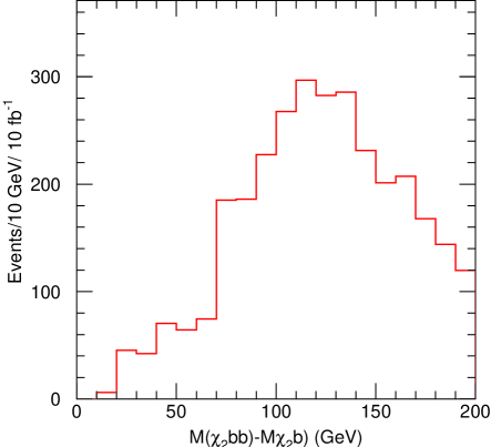
Figure 7: Projection of Figure 6 onto the $m(\tilde{\chi}_{2}^{0}bb)-m(\tilde{\chi}_{2}^{0}b)$ axis.

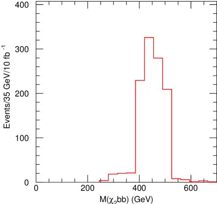
Figure 8: Projection of Figure 6 onto the $m(\tilde{\chi}_{2}^{0}bb)$ axis with the requirement that $100\,{\rm GeV}<m(\tilde{\chi}_{2}^{0}bb)-m(\tilde{\chi}_{2}^{0}b)<140\,{\rm GeV}$.

5 Light Squarks

We now attempt to find evidence for the decay chain $\tilde{q}_{L}\to q\tilde{\chi}_{2}^{0}\to q\tilde{\tau}\tau\to q\tau\tau{\tilde{\chi}_{1}^{0}}$. The rates are not large due to the small branching ratio for the first step, and we can expect considerable combinatorial background from QCD radiation of light quark and gluon jets. The event sample of section 3 is used. In addition we require the presence of a non $b$-jet with $P_{T}>25$ GeV. Events are selected that have reconstructed tau pairs with invarient mass within $\pm 10\,{\rm GeV}$ of peak in Figure 2, and the invariant mass of the tau pair and the jet is formed. This mass distribution is shown in Figure 9. The sign subtracted distribution corresponding to $\tau^{+}\tau^{-}-\tau^{-}\tau^{-}-\tau^{+}\tau^{+}$ is used as it reduces combinatorical background. There should should be an edge at $\sim m_{\tilde{q_{l}}}-m_{\tilde{\chi}_{1}}\sim 400\,{\rm GeV}$. The edge is not sharp — two $\nu_{\tau}$’s and the ${\tilde{\chi}_{1}^{0}}$ are all lost. In addtion the distribtution is contaminated by decays from $\tilde{\chi}_{3}^{0}$ and $\tilde{\chi}_{4}^{0}$. While this distribution is clealy distinct from that shown above where b-jets were used, more work is needed to establish that this could be used to infer information on the light squark mass.

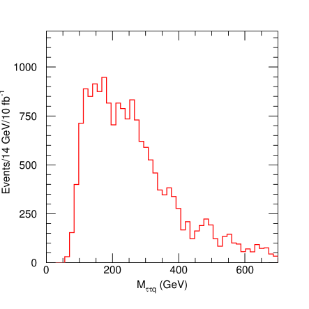
Figure 9: Reconstructed $\tau\tau+{\rm jet}$ mass distribution at for light quark jets.

6 Extraction of $\tilde{q}_{R}$

This analysis is based on the fact that $\tilde{q}_{R}\to q{\tilde{\chi}_{1}^{0}}$ is dominant, so $\tilde{q}_{R}\tilde{q}_{R}$ pair production gives a pair of hard jets and large missing energy. There is no kinematic endpoint, but the $P_{T}$ of the jets provides a measure of the squark mass  [2]. The following cuts were made:

• $\hbox to0.0pt{\hbox to7.95831pt{\hfil/\hfil}\hss}E_{T}>200\,{\rm GeV}$

• 2 jets with $P_{T}>150\,{\rm GeV}$

• No other jet with $p_{T}>25\,{\rm GeV}$

• Transverse sphericity $S_{T}>0.2$

• $\hbox to0.0pt{\hbox to7.95831pt{\hfil/\hfil}\hss}E_{T}>0.2M_{\rm eff}$

• No leptons, No b-jets, No tau jets

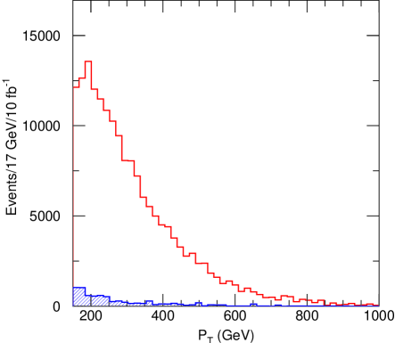
Figure 10: Transverse momentum distribution for jets passing the selection described in section 6. The Standard Model background is shown as the filled histogram.

The transverse momentum distribution of the leading jets is shown in Figure 10. The error on the mass is limited by the systematics of understanding the production dynamics and the SUSY backgrounds. Studies of other cases  [2] have shown that this distribution should enable a precision of $\pm 50\,{\rm GeV}$ to be reached; it might be possible to achieve $\pm 25\,{\rm GeV}$ in a high statistics study.

7 Dilepton Final states

While the light gauginos decay almost entirely into $\tau$’s, the heavy ones can decay via $\tilde{\chi}_{3,4}^{0}\to{\tilde{\ell}}_{l,r}^{\pm}\ell^{\mp}\to\tilde{\chi}_{1,2}^{0}\ell^{+}\ell^{-}$, giving opposite-sign, same-flavor leptons. The largest combined branching is for $\tilde{\chi}_{4}^{0}\to{\tilde{\ell}}_{l}^{\pm}\ell^{\mp}\to{\tilde{\chi}_{1}^{0}}\ell^{+}\ell^{-}$, which gives a dilepton endpoint at

$$M_{\ell\ell}^{\rm max}=\sqrt{(M_{\tilde{\chi}_{4}^{0}}^{2}-M_{{\tilde{\ell}}_{L}}^{2})(M_{{\tilde{\ell}}_{L}}^{2}-M_{{\tilde{\chi}_{1}^{0}}}^{2})\over M_{{\tilde{\ell}}_{L}}^{2}}=163.2\,{\rm GeV}$$

There is of course a large background from leptonic $\tau$ decays, but this can be cancelled statistically by measuring the flavor-subtracted combination $e^{+}e^{-}+\mu^{+}\mu^{-}-e^{\pm}\mu^{\mp}$ as we now demonstrate.

Events were selected to have two leptons with $P_{T}>10\,{\rm GeV}$ and $|\eta|<2.5$ in addition to the jet and $\hbox to0.0pt{\hbox to7.95831pt{\hfil/\hfil}\hss}E_{T}$ cuts described earlier (see Section 3: no tau requirement is applied here). Figure 11 shows the distribution in the $\mu^{+}\mu^{-}$ final state. A clear peak from $Z$ decay is visible that results from $\chi_{3}$ and $\chi_{4}$ decays. The flavor-subtracted combination $e^{+}e^{-}+\mu^{+}\mu^{-}-e^{\pm}\mu^{\mp}$ is shown in Figure 12 and shows an excess extending to $\sim 160$ GeV. Unlike the distributions involvin tau final states, this one can be extrapolated to high luminosity operation which will surely be needed to extract a quantitative result from it.

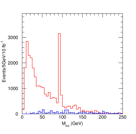
Figure 11: Reconstructed $\mu^{+}\mu^{-}$ mass distribution.. The filled histogram shows the Standard Model background.

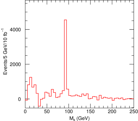
Figure 12: Reconstructed $\mu^{+}\mu^{-}+e^{+}e^{-}-\mu^{+}e^{-}-\mu^{-}e^{+}$ mass distribution.

8 Determining SUSY parameters and Conclusion

The presence of the dijet signal of Section 6 implies that that $m_{\tilde{g}}>m_{\tilde{q}_{R}}$. Likewise the failure to observe a dilepton peak implies that $m_{\tilde{e}_{R}}>m_{\tilde{\chi}_{2}^{0}}$. These results are used together with the assumed errors on the measured quantities to fit the model parameters. The values of the errors on $m_{\tilde{g}}-m_{\tilde{b}}$, $m_{\tilde{g}}$, $m_{\tilde{q_{r}}}$ and the $\tau\tau$ edge are shown in Table 2. We do not use the information from Figures 9 and 12 as we have not estimated the quantitative information that they could give. Two fits are shown since the sign of $\mu$ cannot be determined. This is expected: a change of conventions can replace $\mathop{\rm sgn}\mu$ with $\mathop{\rm sgn}(\tan\beta)$, and $\tan\beta=\pm\infty$ are equivalent.

We assume that the Higgs mass is measured via its decay to two photons. The error on the Higgs mass is likely to be dominated by the theoretical uncertainty on the higher order corrections; both the one-loop and the dominant two-loop effects have been calculated and are large. The present error is probably about $\pm 3\,{\rm GeV}$; this might be reduced to $\pm 1\,{\rm GeV}$ with much more work. The ultimate limit comes from the experimental error, about $\pm 0.2\,{\rm GeV}$. The effect of reducing this error is only apparent in the error of the fitted value of $\tan\beta$ whose error is reduced by approximately a factor of two if $\pm 1\,{\rm GeV}$ error on the Higgs mass is used. The table shows various assumptions for the errors that might be achieved. The numbers in the first column are conservative and will be achieved with the 10 fb^-1 of integrated luminosity shown on the figures. The rightmost column is an estimate of what might ultimately be achievable. We caution the reader that the measurements involving tau’s may not be possible at a luminosity of $10^{34}$ cm^-2 sec^-1 due to pileup effects.

Table 2: Results of the fit for the model parameters. The assumed errors in GeV on the measured quantities are shown for low and high luminosity with two different assumptions about how well the $\tilde{q}_{R}$ mass can be extracted from Figure 10. The fitted values of $m_{0}$ $m_{1/2}$, $\tan\beta$ and $A_{0}$ are given for each case for both signs of $\mu$. The theoretical plus experimental error on the light Higgs mass is assumed to be 3 GeV.

$\cal L$	$10\,{\rm fb}^{-1}$		$100\,{\rm fb}^{-1}$
$\tau\tau$ edge	3.0	3.0	1.2	1.2
$m_{\tilde{g}}-m_{\tilde{b}}$	20.	20.	10.	10.
$m_{\tilde{g}}$	60.	60.	30.	30.
$m_{\tilde{q_{r}}}$	50.	25.	25.	12.
$\mu>0$
$m_{0}$	$232\pm 39$	$228\pm 27$	$230\pm 30$	$227\pm 29$
$m_{1/2}$	$198\pm 14$	$195\pm 11$	$196\pm 10$	$195\pm 9$
$\tan\beta$	$42\pm 7$	$43\pm 6$	$44\pm 5.5$	$44\pm 5$
$A_{0}$	$0\pm 200$	$0\pm 180$	$161\pm 150$	$-60\pm 140$
$\mu<0$
$m_{0}$	$230\pm 37$	$232\pm 26$	$230\pm 26$	$233\pm 26$
$m_{1/2}$	$200\pm 14$	$196\pm 11$	$198\pm 7$	$201\pm 6$
$\tan\beta$	$42\pm 7.3$	$42\pm 7.1$	$45\pm 6.2$	$45\pm 6.1$
$A_{0}$	$0\pm 270$	$0\pm 270$	$-100\pm 210$	$-150\pm 200$

We can see from the table that, despite the fact that the tau momenta cannot be measured directly due to the presence of neutrinos in their decays, we can still expect to infer values of the underlying parameters with errors of better than 10%. Of course these errors are considerably poorer than those that we expect in cases where taus do not have to be used [1]. Our encouraging result arises mainly from the very large statistical sample that LHC can produce for the case considered.

References

- [1] I. Hinchliffe et al. Phys. Rev. D55, 5520 (1997).
- [2] E. Richter-Was et al., ATLAS Internal Note PHYS-No-108.
- [3] I Hinchliffe et al., ATLAS Internal Note PHYS-No-109; G. Polesello, et al., ATLAS Internal Note PHYS-No-111; S. Abdullin, et al., (CMS Collaboration) CMS-NOTE-1998-006.
- [4] F. Gianotti, ATLAS Internal Note PHYS-No-110.
- [5] L. Alvarez-Gaume, J. Polchinski and M.B. Wise, Nucl. Phys. B221, 495 (1983); L. Ibañez, Phys. Lett. 118B, 73 (1982); J.Ellis, D.V. Nanopolous and K. Tamvakis, Phys. Lett. 121B, 123 (1983); K. Inoue et al. Prog. Theor. Phys. 68, 927 (1982); A.H. Chamseddine, R. Arnowitt, and P. Nath, Phys. Rev. Lett., 49, 970 (1982).
- [6] For reviews see, H.P. Nilles, Phys. Rep. 111, 1 (1984); H.E. Haber and G.L. Kane, Phys. Rep. 117, 75 (1985).
- [7] H. Baer, C.-H. Chen, F. Paige, and X. Tata, Phys. Rev. D52, 2746 (1995); Phys. Rev. D53, 6241 (1996).
- [8] L.J. Hall and M. Suzuki, Nucl.Phys. B231, 419 (1984).
- [9] J. Soderqvist, ATL-PHYS-98-122; E. Nagy and A. Mirea, Atlas Note, ATL-PHYS-99-007 (1999),
- [10] F. Paige and S. Protopopescu in Supercollider Physics, p. 41, ed. D. Soper (World Scientific, 1986); H. Baer, F. Paige, S. Protopopescu and X. Tata, in Proceedings of the Workshop on Physics at Current Accelerators and Supercolliders, ed. J. Hewett, A. White and D. Zeppenfeld, (Argonne National Laboratory, 1993).
- [11] ATLAS Collaboration, Technical Proposal, LHCC/P2 (1994).
- [12] CMS Collaboration, Technical Proposal, LHCC/P1 (1994).
- [13] Y. Coadou et al., ATLAS Internal Note ATL-PHYS-98-126.
- [14] T. Sjostrand, Comput.Phys.Commun.82:74-90,1994
- [15] ATLAS DETECTOR AND PHYSICS PERFORMANCE TECHNICAL DESIGN REPORT, Chapter 2, CERN/LHCC 99-15.