hep-ph/9907475 Two-hadron interference fragmentation functions
Part I: general framework

Abstract

We investigate the properties of interference fragmentation functions measurable from the distribution of two hadrons produced in the same jet in the current fragmentation region of a hard process. We discuss the azimuthal angular dependences in the leading order cross section of two-hadron inclusive lepton-nucleon scattering as an example how these interference fragmentation functions can be addressed separately.

I Introduction

Although since the event of Quantum Chromodynamics we do have a renormalisable quantum field theory at hand to describe the interaction of quarks and gluons, we still have to face the fact that there is no rigorous analytical explanation for the confinement of those partons in hadrons. For the investigation of the properties of hadron structure we mainly rely on the information extracted from experimental data on hard scattering processes in form of distribution and fragmentation functions, which can be compared to the predictions of different models. A complete calculation of these objects from first principles, as for instance in lattice gauge theory, is not yet available.

There are three fundamental quark distribution functions (DF) contributing to a hard process at leading order in an expansion in powers of the hard scale $Q$: the momentum distribution $f_{1}$, the longitudinal spin distribution $g_{1}$, and the transversity distribution $h_{1}$. Whereas $f_{1}$ and $g_{1}$ are experimentally rather well measured, presently the transversity distribution $h_{1}$ is still completely unknown. The reason is that it is a chiral-odd object and needs to be combined with a chiral-odd partner to form a (chiral-even) cross section. As such, it is not measurable, for instance, in totally inclusive deep inelastic scattering (DIS) [1]. Together the three fundamental DF characterize the state of quarks in the nucleon with regard to the longitudinal momentum and to its spin to leading power in $Q$. The inclusion of effects related to the transverse momentum of quarks inside the nucleon, and/or to subleading orders in $Q$, results in a larger number of DF [2]. In particular, so called naive time-reversal odd (for sake of brevity “T-odd”) DF arise, in the sense that the constraints due to time-reversal invariance cannot be applied because of, e.g., soft initial-state interactions [3], or chiral symmetry breaking [4], or so-called gluonic poles attributed to asymptotic (large distance) gluon fields [5, 6]. These DF can describe also a polarization of quarks inside unpolarized hadrons.

Information on hadronic structure, complementary to the one given by the DF, is contained in quark fragmentation functions (FF) describing the process of hadronization. To leading order, those functions give the probabilities to find hadrons in a quark. Experimentally known for some species of hadrons is only $D_{1}$, the leading spin-independent FF, which is the direct analogue of $f_{1}$. The basic reason for such a poor knowledge is related to the difficulty of measuring more exclusive channels in hard processes (such as, e.g., semi-inclusive DIS) and/or collecting data sensitive to specific degrees of freedom of the resulting hadrons (transverse momenta, polarization, etc..). However, a new generation of experiments (including both ongoing measurements like HERMES and future projects like COMPASS or experiments at RHIC or ELFE) will have a better ability in identifying final states and will allow for the determination of more subtle effects. In fact, when partially releasing the summation over final states several FF become addressable which are often related to genuine effects due to Final State Interactions (FSI) between the produced hadron and the remnants of the fragmenting quark [2]. In this context, “T-odd” FF naturally arise because the existence of FSI prevents constraints from time-reversal invariance to be applied to the fragmentation process [7, 6]. The usefulness of such an investigation can be demonstrated by considering the so-called Collins effect [8], where a specific asymmetry measurement in the leptoproduction of an unpolarized hadron from a transversely polarized target gives access to $h_{1}$ through the chiral-odd “T-odd” fragmentation function $H_{1}^{\perp}$, which describes the probability for a transversely polarized quark to fragment into an unpolarized hadron.

The presence of FSI allows that in the fragmentation process there are at least two competing channels interfering through a nonvanishing phase. However, as it will be clear in Sec. II, this is not enough to generate “T-odd” FF. A genuine difference in the Lorentz structure of the vertices describing the fragmentation processes is needed. This poses a serious difficulty in modelling the quark fragmentation into one observed hadron because it requires the ability of modelling the FSI between the hadron itself and the rest of the jet, unless one accepts to give up the concept of factorization. Moreover, it was even argued that in this situation summing over all the possible final states could average out any effect [9].

Therefore, in this article we will discuss a specific situation in the hadronization of a current quark, namely the one where two hadrons are observed within the same jet and their momenta are determined. By interference of different production channels FF emerge which are “T-odd”, and can be both chiral even or chiral odd.

For the case of the two hadrons being a pair of pions the resulting FF have been proposed as a tool to investigate the transverse spin dependence of fragmentation. Collins and Ladinsky [10] considered the interference of a scalar resonance with the channel of independent successive two pion production. Jaffe, Jin and Tang [9] proposed the interference of $s$- and $p$-wave production channels, where the relevant phase shifts are essentially known. In the forthcoming paper [11], we will adopt an extended version of the spectator model used in Ref. [12] and will estimate the FF in the case of the pair being a proton and a pion produced either through non-resonant channels or through the Roper ($1440$ MeV) resonance.

This paper is organized as follows. In Sec. II the general conditions for generating “T-odd” FF in semi-inclusive DIS are considered which lead naturally to select the two-hadron semi-inclusive DIS as the simplest case for modelling a complete scenario for the fragmentation process. In Sec. III, FF are defined for the two-hadron semi-inclusive DIS as projections of a proper quark-quark correlation and some relevant kinematics is discussed. In Sec. IV we give a general method to determine all independent leading order two-hadron FF and discuss their symmetry properties. As an example, we demonstrate in Sec. V that asymmetry measurements in two-hadron inclusive lepton-nucleon scattering allow for the isolation of the “T-odd” FF making use of the angular dependences in the leading order cross section. A brief summary and conclusions are given in Sec. VI.

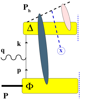
FIG. 1.: Amplitude for a one-hadron semi-inclusive DIS with possible residual interactions in the final state of the detected leading hadron.

II Why a fragmentation into two hadrons?

Let us consider the situation of a one-hadron semi-inclusive DIS, where a quark with momentum $p$ and carrying a fraction $x$ of the target momentum $P$ absorbes a hard photon with momentum $q$ and then hadronizes into a jet which contains a leading hadron with momentum $P_{h}$ eventually detected (Fig. 1). The soft parts that link the initial hard quark $p$ to the target and the final hard quark $k$ to the detected hadron $P_{h}$ indicate the distribution probability of the quark itself inside the target and the transition probability for its hadronization, respectively. They are described by the functions $\Phi(p;P,S)$ and $\Delta(k;P_{h},S_{h})$, that may depend also on the initial and final spin vectors $S,S_{h}$ and contain a sum over all possible residual hadronic states (symbolized by the vertical dashed lines in Fig. 1).

The soft leading hadron can undergo FSI with the sorroundings. In Fig. 1 three symbols represent the three possible classes of models that could describe them. The dark blob indicates mechanisms (at leading or subleading order) that break the factorization hypothesis. The light blob represents interactions with the residual fragments. It is clear that this second class requires non-trivial microscopic modifications of the hadron wave function, in other words it requires the ability of modelling the residual interaction between the outgoing hadron and the rest of the jet in a way that cannot be effectively reabsorbed in the vertex connecting the hard and the soft part. Moreover, it was also argued [9] that the required sum over all possible states of the fragments could average these FSI effects out.

The third symbol, the dashed line originating from the space-time point $X$, represents the most naive class of models, where FSI are simply described by an averaged external potential. Despite its simplicistic approach, this point of view poses serious mathematical difficulties, because the introduction of a potential in principle breaks the translational and rotational invariance of the problem. One could introduce further assumptions about the symmetry properties of the potential to keep these features, but at the price of loosing any contribution to the “T-odd” structure of the amplitude, as it will be clear in the following.

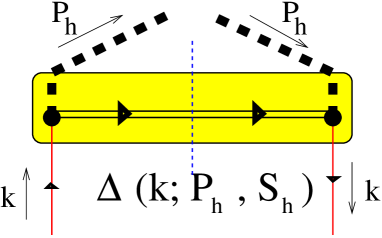
FIG. 2.: Quark-quark correlation function $\Delta$ for the fragmentation of a quark into a hadron. A simple model assumption for the hadronization process is also indicated.

As a pedagogical example, let us consider the oversimplified and unrealistic situation where the detected hadron with mass $M_{h}$ and energy $E_{h}$ is not polarized and does not interact with the rest of the jet; therefore, it is described by the free wave function

$$\psi_{P_{h}}(x)=\sqrt{\frac{M_{h}}{E_{h}}}\;e^{iP_{h}\cdot x}\;u(P_{h})\;,$$ (1)

where $u(P_{h})$ is the free Dirac spinor. In momentum space Eq. (1) reads

$$\psi_{P_{h}}(p)=\frac{1}{(2\pi)^{4}}\;\int d^{\,4\!}p\;e^{-ip\cdot x}\;\psi_{P_{h}}(x)=\sqrt{\frac{M_{h}}{E_{h}}}\;\delta\left(P_{h}-p\right)\;u(P_{h}).$$ (2)

The jet itself is replaced by a spectator system which, again for sake of simplicity, is assumed to be a structureless on-shell scalar diquark with mass $M_{D}$ and momentum $k-P_{h}$ in order to preserve momentum conservation at the vertex. All this amounts to describe the remnants of the fragmentation process with a simple propagator line $\delta((k-P_{h})^{2}-M_{D}^{2})$ for the point-like on-shell scalar diquark $k-P_{h}$. Then, ignoring the inessential $\delta$ functions, the function $\Delta(k;P_{h},S_{h}=0)$ of Fig. 2 becomes

$$\Delta(k;P_{h},S_{h}=0) \sim \frac{-i}{\kern 1.99997ptk\kern-4.49997pt/-m}\;u(P_{h})\overline{u}(P_{h})\;\frac{i}{\kern 1.99997ptk\kern-4.49997pt/-m}$$ (3)

$$= \frac{\kern 1.99997ptk\kern-4.49997pt/+m}{k^{2}-m^{2}}\;(\kern 1.99997ptP\kern-5.59998pt\raisebox{1.29167pt}{/}_{h}+M_{h})\;\frac{\kern 1.99997ptk\kern-4.49997pt/+m}{k^{2}-m^{2}}\;,$$ (4)

where in the second line the usual projector for two free fermion spinors has been used. Eq. (4) can be cast in the following linear combination of all the independent Dirac structures of the process allowed by parity invariance [13, 2],

$$\Delta(k;P_{h},S_{h}=0)=A_{1}M_{h}+A_{2}\kern 1.99997ptP\kern-5.59998pt\raisebox{1.29167pt}{/}_{h}+A_{3}\kern 1.99997ptk\kern-4.49997pt/+\displaystyle{\frac{A_{4}}{M_{h}}}\sigma_{\mu\nu}P_{h}^{\mu}k^{\nu},$$ (5)

where the amplitudes $A_{i}$ are given by

$$A_{1} = \frac{1}{(k^{2}-m^{2})^{2}}\left(k^{2}+m^{2}+2k\cdot P_{h}\frac{m}{M_{h}}\right)$$ (6)

$$A_{2} = {}-\frac{1}{k^{2}-m^{2}}$$ (7)

$$A_{3} = \frac{2\left(P_{h}\cdot k+M_{h}\,m\right)}{(k^{2}-m^{2})^{2}}$$ (8)

$$A_{4} = 0\;.$$ (9)

The function $\Delta(k;P_{h},S_{h}=0)$ must meet the applicable constraints dictated by hermiticity of fields and invariance under time-reversal operations. Hermiticity implies that all $A_{i}$ amplitudes be real. Since the outgoing hadron is described by a free Dirac spinor, time-reversal invariance also implies $A_{4}^{*}=-A_{4}$, from which the usual convention in naming this amplitude time-odd (or “T-odd”) originates. Combining the two constraints gives $A_{4}=0$ in agreement with the previous result deduced just by simple algebra arguments.

This result holds true if in Eq. (2) complex momenta are considered as a simple way to incorporate FSI, as discussed in Ref. [14]. All this amounts to describe the hadron wave function as a plane wave damped uniformly in space through the imaginary part of $P_{h}$. The related symmetric potential, or alternatively the underlying Dirac structure of free spinor assumed for the hadron wave function, do not generate “T-odd” structures in the scattering amplitude.

Let us now allow FSI to proceed through a competing channel having a different spinor structure with respect to the free channel. This example could be cast in the class represented by the light blob of Fig. 1. As a simple test case, we assume for the final hadron spinor the following replacement,

$$u(P_{h})\leftrightarrow u(P_{h})+e^{i\phi}\kern 1.99997ptk\kern-4.49997pt/u(P_{h}),$$ (10)

where $\phi$ is the relative phase between the two channels. Inserting this back into Eq. (4) modifies the $\Delta(k;P_{h},S_{h}=0)$ function according to

$$\Delta(k;P_{h},S_{h}=0)=\left[A_{1}(k^{2}+1)+B_{1}\cos\phi\right]M_{h}+A_{2}(1-k^{2})\kern 1.99997ptP\kern-5.59998pt\raisebox{1.29167pt}{/}_{h}+\left[A_{3}+B_{3}+B_{3}^{\prime}\cos\phi\right]\kern 1.99997ptk\kern-4.49997pt/+\frac{B_{4}\sin\phi}{M_{h}}\sigma_{\mu\nu}P_{h}^{\mu}k^{\nu}\;,$$ (11)

where the new amplitudes $B_{i}$ are given by

$$B_{1} = \frac{1}{(k^{2}-m^{2})^{2}}\left[4\,m\,k^{2}+\frac{2}{M_{h}}k\cdot P_{h}(k^{2}+m^{2})\right]$$ (12)

$$B_{3} = \frac{1}{(k^{2}-m^{2})^{2}}\left(2\,M_{h}\,m\,k^{2}+2\,m^{2}\,k\cdot P_{h}\right)$$ (13)

$$B_{3}^{\prime} = \frac{1}{(k^{2}-m^{2})^{2}}\left[2M_{h}(k^{2}+m^{2})+4\,m\,k\cdot P_{h}\right]$$ (14)

$$B_{4} = \displaystyle{\frac{2M_{h}}{k^{2}-m^{2}}}.$$ (15)

The coefficient of the tensor structure $\sigma_{\mu\nu}$ is now not vanishing provided that the interference between the two channels, namely the phase $\phi$, is not vanishing. In this case, a “T-odd” contribution arises and is maximal for $\phi=\pi/2$.

These simple arguments show that, in order to model “T-odd” FF in one-hadron semi-inclusive processes without giving up factorization, one needs to relate the modifications of the hadron wave function to a realistic microscopic description of the fragmenting jet. Oversimplified assumptions, as in the case of symmetric, mathematically handable, external potentials, can lead to misleading results. Such a hard task suggests that a more convenient way to model occurrence and properties of “T-odd” FF is to look at residual interactions between two hadrons in the same jet, considering the remnant of the jet as a spectator and summing over all its possible configurations. Therefore, in the following the formalism for two-hadron semi-inclusive production and FF will be addressed.

III Quark-quark correlation function for two-hadron production

In the field-theoretical description of hard processes the soft parts connecting quark and gluon lines to hadrons are defined as certain matrix elements of non-local operators involving the quark and gluon fields themselves [15, 16, 17]. In analogy with semi-inclusive hard processes involving one detected hadron in the final state [2], the simplest matrix element for the hadronisation into two hadrons is the quark-quark correlation function describing the decay of a quark with momentum $k$ into two hadrons $P_{1},P_{2}$ (see Fig. 3), namely

$$\Delta_{ij}(k;P_{1},P_{2})=\kern 1.99997pt{\textstyle\sum}\kern-11.00008pt\int_{X}\;\int\frac{d^{\,4\!}\zeta}{(2\pi)^{4}}\;e^{ik\cdot\zeta}\;\langle 0|\,\psi_{i}(\zeta)\,a_{2}^{\dagger}(P_{2})\,a_{1}^{\dagger}(P_{1})\,|X\rangle\;\langle X|\,a_{1}(P_{1})\,a_{2}(P_{2})\,\overline{\psi}_{j}(0)\,|0\rangle\;,$$ (16)

where the sum runs over all the possible intermediate states involving the two final hadrons $P_{1},P_{2}$. For the Fourier transform only the two space-time points $0$ and $\zeta$ matter, i.e. the positions of quark creation and annihilation, respectively. Their relative distance $\zeta$ is the conjugate variable to the quark momentum $k$.

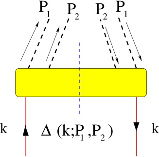
FIG. 3.: Quark-quark correlation function for the fragmentation of a quark into a pair of hadrons.

We choose for convenience the frame where the total pair momentum $P_{h}=P_{1}+P_{2}$ has no transverse component. The constraint to reproduce on-shell hadrons with fixed mass $(P_{1}^{2}=M_{1}^{2},P_{2}^{2}=M_{2}^{2})$ reduces to seven the number of independent degrees of freedom. As shown in Appendix A (where also the light-cone components of a 4-vector are defined), they can conveniently be reexpressed in terms of the light-cone component of the hadron pair momentum, $P_{h}^{-}$, of the light-cone fraction of the quark momentum carried by the hadron pair, $z_{h}=P_{h}^{-}/k^{-}=z_{1}+z_{2}$, of the fraction of hadron pair momentum carried by each individual hadron, $\xi=z_{1}/z_{h}=1-z_{2}/z_{h}$, and of the four independent invariants that can be formed by means of the momenta $k,P_{1},P_{2}$ at fixed masses $M_{1},M_{2}$, i.e.

$$\tau_{h}=k^{2}\;,\quad\sigma_{h}=2\,k\cdot(P_{1}+P_{2})\equiv 2\,k\cdot P_{h}\;,\quad\sigma_{d}=2\,k\cdot(P_{1}-P_{2})\equiv 4\,k\cdot R\;,\quad M_{h}^{2}=\left(P_{1}+P_{2}\right)^{2}\equiv P_{h}^{2}\;,$$ (17)

where we define the vector $R=(P_{1}-P_{2})/2$ for later use.

By generalizing the Collins-Soper light-cone formalism [16] for fragmentation into multiple hadrons [10, 9], the cross section for two-hadron semi-inclusive emission can be expressed in terms of specific Dirac projections of $\Delta(z_{h},\xi,P_{h}^{-},\tau_{h},\sigma_{h},M_{h}^{2},\sigma_{d})$ after integrating over the (hard-scale suppressed) light-cone component $k^{+}$ and, consequently, taking $\zeta$ as light-like [2], i.e.

$$\Delta^{[\Gamma]}=\frac{1}{4z_{h}}\left.\int dk^{+}\;\mbox{Tr}[\Delta\Gamma]\right|_{\zeta^{-}=0}=\frac{1}{4z_{h}}\int dk^{+}\;\int dk^{-}\;\delta\left(k^{-}-\frac{P_{h}^{-}}{z_{h}}\right)\;\mbox{Tr}[\Delta\Gamma]\;.$$ (18)

The function $\Delta^{[\Gamma]}$ now depends on five variables, apart from the Lorentz structure of the Dirac matrix $\Gamma$. In order to make this more explicit and to reexpress the set of variables in a more convenient way, let us rewrite the integrations in Eq. (18) in a covariant way using

$$2\,P_{h}^{-}=\frac{d\sigma_{h}}{dk^{+}},\qquad 2\,k^{+}=\frac{d\tau_{h}}{dk^{-}},$$ (19)

and the relation

$$\frac{1}{2k^{+}}\delta\left(k^{-}-\frac{P_{h}^{-}}{z_{h}}\right)=\delta\left(2k^{+}k^{-}-\frac{2k^{+}P_{h}^{-}}{z_{h}}\right)=\delta\left(\tau_{h}+{\vec{k}}_{\scriptscriptstyle T}^{\,2}-\frac{\sigma_{h}}{z_{h}}+\frac{M_{h}^{2}}{z_{h}^{2}}\right)$$ (20)

which leads to the result

$$\Delta^{[\Gamma]}(z_{h},\xi,{\vec{k}}_{\scriptscriptstyle T}^{\,2},M_{h}^{2},\sigma_{d})=\int d\sigma_{h}\,d\tau_{h}\;\delta\left(\tau_{h}+{\vec{k}}_{\scriptscriptstyle T}^{\,2}-\frac{\sigma_{h}}{z_{h}}+\frac{M_{h}^{2}}{z_{h}^{2}}\right)\;\frac{\mbox{Tr}[\Delta(z_{h},\xi,P_{h}^{-},\tau_{h},\sigma_{h},M_{h}^{2},\sigma_{d})\;\Gamma]}{8z_{h}P_{h}^{-}}\;,$$ (21)

where the dependence on the transverse quark momentum ${\vec{k}}_{\scriptscriptstyle T}^{\,2}$ through $\sigma_{h}$ is made explicit by means of Eqs. (A16) and (A19).

Using Eq. (A) makes it possible to reexpress $\Delta^{[\Gamma]}$ as a function of $z_{h}$, $\xi$, ${\vec{k}}_{\scriptscriptstyle T}^{\,2}$ and ${\vec{R}}_{\scriptscriptstyle T}^{\,2}$, ${\vec{k}}_{\scriptscriptstyle T}\cdot{\vec{R}}_{\scriptscriptstyle T}$, where ${\vec{R}}_{\scriptscriptstyle T}$ is (half of) the transverse momentum between the two hadrons in the considered frame. In this manner $\Delta^{[\Gamma]}$ depends on how much of the fragmenting quark momentum is carried by the hadron pair $(z_{h})$, on the way this momentum is shared inside the pair $(\xi)$, and on the “geometry” of the pair, namely on the relative momentum of the two hadrons $({\vec{R}}_{\scriptscriptstyle T}^{\,2})$ and on the relative orientation between the pair plane and the quark jet axis (${\vec{k}}_{\scriptscriptstyle T}^{\,2}$, ${\vec{k}}_{\scriptscriptstyle T}\cdot{\vec{R}}_{\scriptscriptstyle T}$, see also Fig. 4).

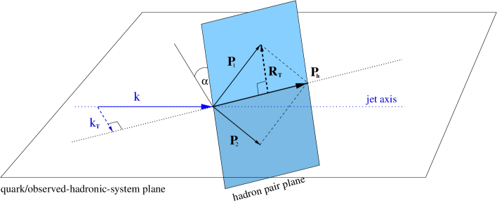
FIG. 4.: Kinematics for a fragmenting quark jet containing a pair of leading hadrons.

IV Analysis of interference fragmentation functions

If the polarizations of the two final hadrons are not observed, the quark-quark correlation $\Delta(k;P_{1},P_{2})$ of Eq. (16) can be generally expanded, according to hermiticity and parity invariance, as a linear combination of the independent Dirac structures of the process

$$\Delta(k;P_{1},P_{2}) = B_{1}\,\left(M_{1}+M_{2}\right)+B_{2}\,\kern 1.99997ptP\kern-5.59998pt\raisebox{1.29167pt}{/}_{1}+B_{3}\,\kern 1.99997ptP\kern-5.59998pt\raisebox{1.29167pt}{/}_{2}+B_{4}\,\kern 1.99997ptk\kern-4.49997pt/$$ (24)

$${}+\frac{B_{5}}{M_{1}}\,\sigma^{\mu\nu}P_{1\mu}k_{\nu}{}+\frac{B_{6}}{M_{2}}\,\sigma^{\mu\nu}P_{2\mu}k_{\nu}{}+\frac{B_{7}}{M_{1}+M_{2}}\,\sigma^{\mu\nu}P_{1\mu}P_{2\nu}$$

$${}+\frac{B_{8}}{M_{1}M_{2}}\,\gamma_{5}\,\epsilon^{\mu\nu\rho\sigma}\gamma_{\mu}P_{1\nu}P_{2\rho}k_{\sigma}\;.$$

Symmetry constraints are obtained in the form

$$\gamma_{0}\,\Delta^{\dagger}(k;P_{1},P_{2})\,\gamma_{0} = \Delta(k;P_{1},P_{2})\qquad\qquad\mbox{from hermiticity,}$$ (26)

$$\gamma_{0}\,\Delta(\tilde{k};\tilde{P}_{1},\tilde{P}_{2})\,\gamma_{0} = \Delta(k;P_{1},P_{2})\qquad\qquad\mbox{from parity invariance,}$$ (27)

$$\left(\gamma_{5}C\,\Delta(\tilde{k};\tilde{P}_{1},\tilde{P}_{2})\,C^{\dagger}\gamma_{5}\right)^{\ast} = \Delta(k;P_{1},P_{2})\quad\qquad\mbox{from time-reversal invariance}\;,$$ (28)

where $\tilde{a}=(a^{0},-\vec{a})$ and $C=i\,\gamma^{2}\,\gamma^{0}$. From the hermiticity of the fields it follows that

$$B_{i}^{*}=B_{i}\qquad\mbox{for}\quad i=1,..,12$$ (29)

and, if constraints from time-reversal invariance can be applied, that

$$B_{i}^{*}=B_{i}\qquad\mbox{for}\quad i=1,..,4\qquad\qquad B_{i}^{*}=-B_{i}\qquad\mbox{for}\quad i=5,..,8\;,$$ (30)

which means in that case $B_{5}=B_{6}=B_{7}=B_{8}=0$, i.e. terms involving $B_{5},..,B_{8}$ are naive “T-odd”.

Inserting the ansatz (24) in Eq. (21) and reparametrizing the momenta $k,P_{1},P_{2}$ with the indicated new set of variables, we get the following Dirac projections

$$\Delta^{[\gamma^{-}]}(z_{h},\xi,{\vec{k}}_{\scriptscriptstyle T}^{\,2},{\vec{R}}_{\scriptscriptstyle T}^{\,2},{\vec{k}}_{\scriptscriptstyle T}\cdot{\vec{R}}_{\scriptscriptstyle T}) \equiv D_{1}(z_{h},\xi,{\vec{k}}_{\scriptscriptstyle T}^{\,2},{\vec{R}}_{\scriptscriptstyle T}^{\,2},{\vec{k}}_{\scriptscriptstyle T}\cdot{\vec{R}}_{\scriptscriptstyle T})$$ (31)

$$= \frac{1}{2z_{h}}\int[d\sigma_{h}d\tau_{h}]\ \left[B_{2}\,\xi+B_{3}\,(1-\xi)+B_{4}\,\frac{1}{z_{h}}\right]$$ (32)

$$\Delta^{[\gamma^{-}\gamma_{5}]}(z_{h},\xi,{\vec{k}}_{\scriptscriptstyle T}^{\,2},{\vec{R}}_{\scriptscriptstyle T}^{\,2},{\vec{k}}_{\scriptscriptstyle T}\cdot{\vec{R}}_{\scriptscriptstyle T}) \equiv \frac{\epsilon_{\scriptscriptstyle T}^{ij}\,R_{{\scriptscriptstyle T}i}\,k_{{\scriptscriptstyle T}j}}{M_{1}\,M_{2}}\;G_{1}^{\perp}(z_{h},\xi,{\vec{k}}_{\scriptscriptstyle T}^{\,2},{\vec{R}}_{\scriptscriptstyle T}^{\,2},{\vec{k}}_{\scriptscriptstyle T}\cdot{\vec{R}}_{\scriptscriptstyle T})$$ (33)

$$= \frac{\epsilon_{\scriptscriptstyle T}^{ij}\,R_{{\scriptscriptstyle T}i}\,k_{{\scriptscriptstyle T}j}}{M_{1}\,M_{2}}\;\frac{1}{2z_{h}}\int[d\sigma_{h}d\tau_{h}]\ \left[-B_{8}\right]$$ (34)

$$\Delta^{[i\sigma^{i-}\gamma_{5}]}(z_{h},\xi,{\vec{k}}_{\scriptscriptstyle T}^{\,2},{\vec{R}}_{\scriptscriptstyle T}^{\,2},{\vec{k}}_{\scriptscriptstyle T}\cdot{\vec{R}}_{\scriptscriptstyle T}) \equiv {\epsilon_{\scriptscriptstyle T}^{ij}R_{{\scriptscriptstyle T}j}\over M_{1}+M_{2}}\,H_{1}^{{<\kern-2.10002pt{\scriptscriptstyle)}}}(z_{h},\xi,{\vec{k}}_{\scriptscriptstyle T}^{\,2},{\vec{R}}_{\scriptscriptstyle T}^{\,2},{\vec{k}}_{\scriptscriptstyle T}\cdot{\vec{R}}_{\scriptscriptstyle T})+{\epsilon_{\scriptscriptstyle T}^{ij}k_{{\scriptscriptstyle T}j}\over M_{1}+M_{2}}\,H_{1}^{\perp}(z_{h},\xi,{\vec{k}}_{\scriptscriptstyle T}^{\,2},{\vec{R}}_{\scriptscriptstyle T}^{\,2},{\vec{k}}_{\scriptscriptstyle T}\cdot{\vec{R}}_{\scriptscriptstyle T})$$ (35)

$$= {\epsilon_{\scriptscriptstyle T}^{ij}R_{{\scriptscriptstyle T}j}\over M_{1}+M_{2}}\,\frac{1}{2z_{h}}\int[d\sigma_{h}d\tau_{h}]\,\left[-B_{5}\left(\frac{M_{1}+M_{2}}{z_{h}M_{1}}\right)+B_{6}\left(\frac{M_{1}+M_{2}}{z_{h}M_{2}}\right)-B_{7}\right]$$ (37)

$${}+{\epsilon_{\scriptscriptstyle T}^{ij}k_{{\scriptscriptstyle T}j}\over M_{1}+M_{2}}\,\frac{1}{2z_{h}}\int[d\sigma_{h}d\tau_{h}]\,\left[B_{5}\,\xi\left(\frac{M_{1}+M_{2}}{M_{1}}\right)+B_{6}\,(1-\xi)\left(\frac{M_{1}+M_{2}}{M_{2}}\right)\right]\;,$$

where $\epsilon_{\scriptscriptstyle T}^{\mu\nu}\equiv\epsilon^{-+\mu\nu}$ (such that $i,j$ are transverse indices) and

$$\int[d\sigma_{h}d\tau_{h}]\equiv\int d\sigma_{h}\,d\tau_{h}\;\delta\left(\tau_{h}+{\vec{k}}_{\scriptscriptstyle T}^{\,2}-\frac{\sigma_{h}}{z_{h}}+\frac{M_{h}^{2}}{z_{h}^{2}}\right)\;.$$ (38)

Transverse 4-vectors are defined as $a_{\scriptscriptstyle T}^{\mu}=g_{\scriptscriptstyle T}^{\mu\nu}\,a_{\nu}=[0,0,\vec{a}_{\scriptscriptstyle T}]$ (with $g_{\scriptscriptstyle T}^{\mu\nu}=g^{\mu\nu}-n_{+}^{\mu}n_{-}^{\nu}-n_{+}^{\nu}n_{-}^{\mu}$).

The functions $D_{1}$, $G_{1}^{\perp}$, $H_{1}^{{<\kern-2.10002pt{\scriptscriptstyle)}}}$, $H_{1}^{\perp}$ are the FF that arise to leading order in $1/Q$ for the fragmentation of a current quark into two unpolarized hadrons inside the same jet. The different Dirac structures used in the projections are related to different spin states of the fragmenting quark and lead to a nice probabilistic interpretation [2]. As illustrated in Fig. 5, $D_{1}$ is the probability for an unpolarized quark to produce a pair of unpolarized hadrons; $G_{1}^{\perp}$ is the difference of probabilities for a longitudinally polarized quark with opposite chiralities to produce a pair of unpolarized hadrons; $H_{1}^{{<\kern-2.10002pt{\scriptscriptstyle)}}}$ and $H_{1}^{\perp}$ both are differences of probabilities for a transversely polarized quark with opposite spins to produce a pair of unpolarized hadrons.

The interference functions $G_{1}^{\perp}$, $H_{1}^{{<\kern-2.10002pt{\scriptscriptstyle)}}}$ and $H_{1}^{\perp}$ are (naive) “T-odd”. In fact, the probability for an anyway polarized quark with observed transverse momentum to fragment into unpolarized hadrons is nonvanishing only if there are residual interactions in the final state. In this case, constraints from time-reversal invariance cannot be applied, i.e. the condition (30) does not apply, and indeed the projections (34),(37) are nonvanishing. A measure of these functions would directly give the size and importance of such FSI inside the jet.

$G_{1}^{\perp}$ is chiral even; it has a counterpart in the FF for one-hadron semi-inclusive production. In that case, from the $\Delta^{[\gamma^{-}]}$ projection a “T-odd” FF arises, named $D_{1T}^{\perp}$, which describes the probability for an unpolarized quark with observed transverse momentum to fragment in a transversely polarized hadron [2]. It is known also in a different context [18] that the similarity is recovered by substituting an axial vector (the hadron transverse spin) with a vector (the momentum of a second detected hadron) and by balancing this change in parity with the introduction of the quark polarization.

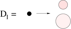
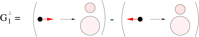
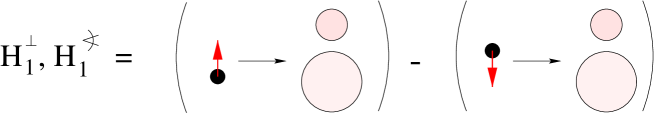
FIG. 5.: Probabilistic interpretation for the leading order FF arising in the decay of a current quark into a pair of unpolarized hadrons.

The functions $H_{1}^{{<\kern-2.10002pt{\scriptscriptstyle)}}}$ and $H_{1}^{\perp}$ are chiral odd and can, therefore, be identified as the chiral partners needed to access the transversity $h_{1}$, as it will be shown in Sec. V. Given their probabilistic interpretation, they can be considered as a sort of “double” Collins effect [8]. They differ just by geometrical weighting factors that are selectively sensitive either to the relative momentum of the final hadrons $({\vec{R}}_{\scriptscriptstyle T})$ or to the relative orientation of the total pair momentum with respect to the jet axis (${\vec{k}}_{\scriptscriptstyle T}$, see also Fig. 4).

V Azimuthal asymmetries in two-hadron inclusive DIS

We discuss the two-hadron inclusive DIS cross section for the general situation of any two unpolarized hadrons produced in the quark current jet as an example for a hard process in which interference FF can be measured. We demonstrate briefly that asymmetry measurements allow for the isolation of each individual interference FF convoluted with a specific DF. Only leading order $(1/Q)^{0}$ effects are discussed and we do not consider QCD corrections, i.e. we focus on tree-level $(\alpha_{s})^{0}$.

To leading order the hadron tensor of the process, including quarks and anti-quarks, is (see Fig. 6 for the definition of momenta)

$$2M\,{\cal W}^{\mu\nu} = \int dp^{-}\,dk^{+}\,d^{\,2}{\vec{p}}_{\scriptscriptstyle T}\,d^{\,2}{\vec{k}}_{\scriptscriptstyle T}\;\delta^{2}\!\left({\vec{p}}_{\scriptscriptstyle T}+{\vec{q}}_{\scriptscriptstyle T}-{\vec{k}}_{\scriptscriptstyle T}\right)$$ (44)

$$\hskip 73.97716pt\times\mbox{Tr}\big{[}\;\Phi(p;P,S)\;\gamma^{\mu}\;\Delta(k;P_{1},P_{2})\;\gamma^{\nu}\;\big{]}\Big{|}_{\begin{array}[]{l}p^{+}=xP^{+}\\ k^{-}=P_{h}^{-}/z_{h}\end{array}}+\left(\begin{array}[]{c}q\leftrightarrow-q\\ \mu\leftrightarrow\nu\end{array}\right)\;,$$

where $M$ is the target hadron mass.

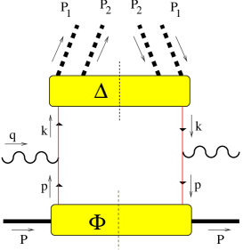
FIG. 6.: Quark diagram contributing in leading order to two-hadron inclusive DIS when both hadrons are in the same quark current jet. There is a similar diagram for anti-quarks.

The quark-quark correlation functions $\Phi$ for the (spin-1/2) target hadron is defined (in the light-cone gauge) as

$$\Phi_{mn}(p;P,S)=\int\frac{d^{\,4\!}\zeta}{(2\pi)^{4}}\;e^{ip\cdot\zeta}\;\langle{P,S|\,\overline{\psi}_{n}(0)\psi_{m}(\zeta)\,|P,S}\rangle\;.$$ (45)

Using Lorentz invariance, hermiticity, and parity invariance, the (partly integrated) correlation function $\Phi$ is parametrized in terms of DF as

$$\Phi(x,{\vec{p}}_{\scriptscriptstyle T}) \equiv \left.\int dp^{-}\ \Phi(p;P,S)\right|_{p^{+}=xP^{+}}\!\!\!\!=\frac{M}{2P^{+}}\,\Biggl{\{}f_{1}\,\frac{\kern 1.99997ptP\kern-5.59998pt\raisebox{1.29167pt}{/}}{M}+f_{1T}^{\perp}\,\epsilon_{\mu\nu\rho\sigma}\gamma^{\mu}\frac{P^{\nu}p_{\scriptscriptstyle T}^{\rho}S_{{\scriptscriptstyle T}}^{\sigma}}{M^{2}}-\left(\lambda\,g_{1L}+\frac{({\vec{p}}_{\scriptscriptstyle T}\cdot{\vec{S}}_{{\scriptscriptstyle T}})}{M}\,g_{1T}\right)\frac{\kern 1.99997ptP\kern-5.59998pt\raisebox{1.29167pt}{/}\gamma_{5}}{M}$$ (47)

$$-h_{1T}\,\frac{i\sigma_{\mu\nu}\gamma_{5}S_{{\scriptscriptstyle T}}^{\mu}P^{\nu}}{M}-\left(\lambda\,h_{1L}^{\perp}+\frac{({\vec{p}}_{\scriptscriptstyle T}\cdot{\vec{S}}_{{\scriptscriptstyle T}})}{M}\,h_{1T}^{\perp}\right)\,\frac{i\sigma_{\mu\nu}\gamma_{5}p_{\scriptscriptstyle T}^{\mu}P^{\nu}}{M^{2}}+h_{1}^{\perp}\,\frac{\sigma_{\mu\nu}p_{\scriptscriptstyle T}^{\mu}P^{\nu}}{M^{2}}\Biggl{\}},$$

where the DF depend on the usual invariant $x=Q^{2}/(2P\cdot q)$ and the quark transverse momentum ${\vec{p}}_{\scriptscriptstyle T}$ [2, 6]. The polarization state of the target is fully specified by the light-cone helicity $\lambda=M\,S^{+}/P^{+}$ and the transverse spin $\vec{S}_{\scriptscriptstyle T}$ of the target hadron. The quark-quark correlation function $\Delta$ has the structure discussed in Sec. IV.

The definitions of DF and FF are given in a reference frame where the target hadron momentum $P$ and the momentum of the produced hadron pair $P_{h}$ have no transverse components, i.e. $\vec{P}_{\scriptscriptstyle T}=\vec{P}_{h{\scriptscriptstyle T}}=0$ and $\vec{q}_{\scriptscriptstyle T}\neq 0$ (see Appendix A).

For the analysis of the cross section of the full DIS process, however, a different frame turns out to be more useful. Angular dependences are conveniently expressed in a frame where the target hadron momentum $P$ and the photon momentum $q$ are collinear: transverse components in this frame are indicated with a $\perp$ subscript, thus $\vec{P}_{\perp}=\vec{q}_{\perp}=0$ and $\vec{P}_{h\perp}\neq 0$ (see Fig. 7 and Refs. [2, 6] for more details about the kinematics). The cross sections should be kept differential in $d^{\,2\!}\vec{P}_{h\perp}$ for which the relation $\vec{q}_{\scriptscriptstyle T}=-\vec{P}_{h\perp}/z_{h}$ holds.

All azimuthal angles are defined with respect to $\hat{l}_{\perp}^{\mu}$, which is the normalized perpendicular part of the incoming lepton momentum $l$ such that, for a generic perpendicular 4-vector $a$,

$$\hat{l}_{\perp}\cdot a_{\perp} = -|{\vec{a}}_{\perp}|\cos\phi_{a},$$ (48)

$$\epsilon^{\mu\nu}_{\perp}\hat{l}_{\perp\mu}a_{\perp\nu} = |{\vec{a}}_{\perp}|\sin\phi_{a},$$ (49)

where $\epsilon^{\mu\nu}_{\perp}=\epsilon^{\mu\nu\rho\sigma}\,q_{\rho}\,P_{\sigma}/(P\cdot q)$. Frequently, we will use the normalized perpendicular vector $\hat{h}^{\mu}=P_{h\perp}^{\mu}/|{\vec{P}}_{h\perp}|=g_{\perp}^{\mu\nu}P_{h\nu}/|{\vec{P}}_{h\perp}|$ (with $g^{\mu\nu}_{\perp}=g^{\mu\nu}-(Q^{2}P^{\mu}P^{\nu})/(P\cdot q)$).

A comment has to be made about the definition of the perpendicular vectors $R_{\perp}$ and $S_{\perp}$, which are obtained from the transverse 4-vectors $R_{\scriptscriptstyle T}$ and $S_{\scriptscriptstyle T}$ by transforming with an appropriate Lorentz boost to the frame where $P$ and $q$ are collinear. Only the components which are perpendicular in the new frame are kept. Technically this procedure amounts to $R_{\perp}^{\mu}=g_{\perp}^{\mu\nu}\;R_{{\scriptscriptstyle T}\,\nu}=g_{\perp}^{\mu\nu}\;\left(g_{\nu\rho}^{\scriptscriptstyle T}\;R^{\rho}\right)$ and similar for $S_{\perp}$.

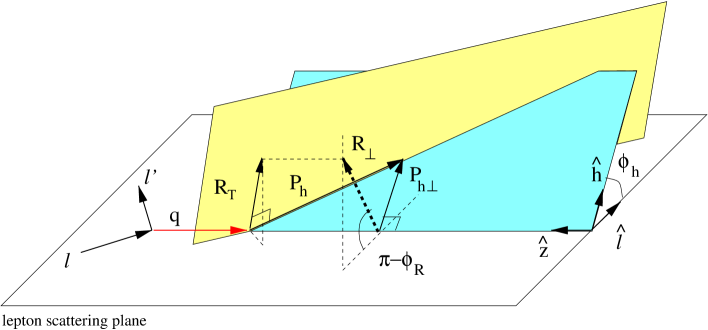
FIG. 7.: Kinematics for two-hadron inclusive leptoproduction. The lepton scattering plane is determined by the momenta $l$, $l^{\prime}$. The momentum $P_{h}=P_{1}+P_{2}$ of the hadron pair represents the intersection between the lightly shaded hadron-pair plane (containing $\vec{R}_{\scriptscriptstyle T}$) and the shaded plane that defines the azimuthal dependence of the pair emission. $\vec{R}_{\perp}$ and $\vec{P}_{h\,\perp}$ lie in a plane perpendicular to the scattering one, where $P,q$ are collinear ($\vec{P}_{\perp}=\vec{q}_{\perp}=0$).

The differential cross section for the process under consideration is obtained by contraction of the hadron tensor with the standard lepton tensor, and involves convolution integrals of DF and FF of the generic form 

$${\cal F}\left[w({\vec{p}}_{\scriptscriptstyle T},{\vec{k}}_{\scriptscriptstyle T})\;f\,D\right]\equiv\;\sum_{a}e_{a}^{2}\;\int d^{\,2}{\vec{p}}_{\scriptscriptstyle T}\;d^{\,2}{\vec{k}}_{\scriptscriptstyle T}\;\delta^{2}({\vec{p}}_{\scriptscriptstyle T}+{\vec{q}}_{\scriptscriptstyle T}-{\vec{k}}_{\scriptscriptstyle T})\;w({\vec{p}}_{\scriptscriptstyle T},{\vec{k}}_{\scriptscriptstyle T})\;f^{a}(x,{\vec{p}}_{\scriptscriptstyle T})\,D^{a}(z_{h},\xi,{\vec{k}}_{\scriptscriptstyle T}^{\,2},{\vec{R}}_{\scriptscriptstyle T}^{\,2},{\vec{k}}_{\scriptscriptstyle T}\cdot{\vec{R}}_{\scriptscriptstyle T})\;,$$ (50)

where $w({\vec{p}}_{\scriptscriptstyle T},{\vec{k}}_{\scriptscriptstyle T})$ is a weight function and the sum runs over all quark (and anti-quark) flavors, with $e_{a}$ the electric charges of the quarks. In the cross sections we will encounter the following functions of the lepton invariant $y=(P\cdot q)/(P\cdot l)\approx q^{-}/l^{-}$:

$$A(y)=\left(1-y+\frac{1}{2}y^{2}\right),\quad B(y)=(1-y),\quad C(y)=y(2-y).$$ (51)

In the following we discuss some particularly interesting terms of the cross section for special cases of beam and target polarizations. The full cross section is listed in Appendix B. However, parts that cancel in taking differences of cross sections with reversed polarizations are not shown.

With a polarized beam ($L$), with helicity $\lambda_{e}$, scattering on an unpolarized target ($O$), the cross section

$$\frac{d\sigma(\ell H\to\ell^{\prime}h_{1}h_{2}X)_{LO}}{d\Omega\,dx\,dz_{h}\,d\xi\,d^{\,2\!}{\vec{P}}_{h\perp}\,d^{\,2\!}{\vec{R}}_{\perp}}\propto\Bigg{\{}\ldots-\lambda_{e}\;|{\vec{R}}_{\perp}|\;\;C(y)\;\sin(\phi_{h}-\phi_{R})\;{\cal F}\left[\,{\vec{\hat{h}}}\!\cdot\!\vec{k}_{\scriptscriptstyle T}\,\frac{f_{1}\,G_{1}^{\perp}}{2M_{1}M_{2}}\right]\Bigg{\}}$$ (52)

is sensitive to a convolution of the unpolarized DF $f_{1}$ with $G_{1}^{\perp}$. The azimuthal angles $\phi_{h},\phi_{R}$ are shown in Fig. 7, while $\Omega$ represents the solid angle of the scattered lepton. Repeating the measurement with reversed beam helicity $\lambda_{e}$ and taking the difference of the cross sections singles out the term of interest.

A very similar term occurs in the cross section for an unpolarized beam ($O$) scattering on a longitudinally polarized target ($L$)

$$\frac{d\sigma(\ell H\to\ell^{\prime}h_{1}h_{2}X)_{OL}}{d\Omega\,dx\,dz_{h}\,d\xi\,d^{\,2\!}{\vec{P}}_{h\perp}\,d^{\,2\!}{\vec{R}}_{\perp}} \propto \Bigg{\{}\ldots{}-\lambda\;|{\vec{R}}_{\perp}|\;A(y)\;\sin(\phi_{h}-\phi_{R})\;{\cal F}\left[\,{\vec{\hat{h}}}\!\cdot\!\vec{k}_{\scriptscriptstyle T}\,\frac{g_{1}\,G_{1}^{\perp}}{M_{1}M_{2}}\right]+\ldots\Bigg{\}}\;,$$ (53)

where the FF $G_{1}^{\perp}$ is convoluted with the polarized DF $g_{1}$. The azimuthal angular dependence is the same as before. For this experiment, reversing the polarization of the target is not sufficient to single out the interesting term, since the full cross section (cf. Appendix B) contains more contributions which do not cancel in the difference. One has to analyze the azimuthal angular dependence, which is unique for each contributing term.

With a transversely polarized target ($T$) and unpolarized beam ($O$), the cross section contains the contributions

$$\frac{d\sigma(\ell H\to\ell^{\prime}h_{1}h_{2}X)_{OT}}{d\Omega\,dx\,dz_{h}\,d\xi\,d^{\,2\!}{\vec{P}}_{h\perp}\,d^{\,2\!}{\vec{R}}_{\perp}} \propto \Bigg{\{}\ldots{}+|{\vec{S}}_{\perp}|\;B(y)\;\sin(\phi_{h}+\phi_{S}){\cal F}\left[\,{\vec{\hat{h}}}\!\cdot\!\vec{k}_{\scriptscriptstyle T}\,\frac{h_{1}\,H_{1}^{\perp}}{M_{1}+M_{2}}\right]$$ (55)

$${}+|{\vec{S}}_{\perp}|\;|{\vec{R}}_{\perp}|\;B(y)\;\sin(\phi_{R}+\phi_{S})\;{\cal F}\left[\frac{h_{1}\,H_{1}^{{<\kern-2.10002pt{\scriptscriptstyle)}}}}{M_{1}+M_{2}}\right]+\ldots\Bigg{\}}\;,$$

which involve the transversity DF $h_{1}$, and the FF $H_{1}^{\perp}$ and $H_{1}^{{<\kern-2.10002pt{\scriptscriptstyle)}}}$, respectively. The experimental situation is analogous to the one proposed to access the transversity $h_{1}$ in one-hadron inclusive DIS via the so-called Collins effect [8]. In the process under consideration, two contributions of similar kind arise which can be analyzed separately using their different kinematical signatures. In fact, asymmetry measurements can firstly be done, that isolate both contributions in Eq. (55). Then, the analysis of the asymmetry produced by interchanging the relative position of the hadron pair (i.e., by flipping $\vec{R}$ by $180^{\rm o}$) isolates the convolution containing $H_{1}^{{<\kern-2.10002pt{\scriptscriptstyle)}}}$. This second term is interesting, since the absence of a $\vec{k}_{\scriptscriptstyle T}-$ (or $\vec{p}_{\scriptscriptstyle T}-$) dependent weight factor in the convolution integral allows for a nonvanishing integration of the differential cross section over $d^{\,2\!}\vec{P}_{h\perp}$, such that the the convolution turns into a product of DF and FF

$$\int d^{\,2\!}\vec{P}_{h\perp}\;{\cal F}\left[\frac{h_{1}\,H_{1}^{{<\kern-2.10002pt{\scriptscriptstyle)}}}}{M_{1}+M_{2}}\right] = \frac{z_{h}^{2}}{M_{1}+M_{2}}\;\sum_{a}e_{a}^{2}\;\int d^{\,2}{\vec{p}}_{\scriptscriptstyle T}\;h_{1}^{a}(x,{\vec{p}}_{\scriptscriptstyle T})\;\;\int d^{\,2}{\vec{k}}_{\scriptscriptstyle T}\;H_{1}^{{<\kern-2.10002pt{\scriptscriptstyle)}}\,a}(z_{h},\xi,{\vec{k}}_{\scriptscriptstyle T}^{\,2},{\vec{R}}_{\scriptscriptstyle T}^{\,2},{\vec{k}}_{\scriptscriptstyle T}\cdot{\vec{R}}_{\scriptscriptstyle T})$$ (56)

$$= \frac{z_{h}^{2}}{M_{1}+M_{2}}\;\sum_{a}e_{a}^{2}\;\;\;h_{1}^{a}(x)\;\;\;H_{1}^{{<\kern-2.10002pt{\scriptscriptstyle)}}\,a}(z_{h},\xi,{\vec{R}}_{\scriptscriptstyle T}^{\,2}).$$ (57)

The corresponding experimental situation is favorable, since less kinematical variables have to be determined and the quantity of interest depends on $z_{h}$, $\xi$ and ${\vec{R}}_{\scriptscriptstyle T}^{\,2}$ only. Note, however, that terms in $H_{1}^{{<\kern-2.10002pt{\scriptscriptstyle)}}}(z_{h},\xi,{\vec{k}}_{\scriptscriptstyle T}^{\,2},{\vec{R}}_{\scriptscriptstyle T}^{\,2},{\vec{k}}_{\scriptscriptstyle T}\cdot{\vec{R}}_{\scriptscriptstyle T})$ with odd powers of ${\vec{k}}_{\scriptscriptstyle T}$, like for instance ${\vec{k}}_{\scriptscriptstyle T}\cdot{\vec{R}}_{\scriptscriptstyle T}$, do not survive the symmetric integration over $d^{\,2}{\vec{k}}_{\scriptscriptstyle T}$.

VI Summary and Outlooks

In this paper we have investigated the general properties of interference fragmentation functions (FF) that arise from the distribution of two hadrons produced in the same jet in the current fragmentation region of a hard process, e.g., in two-hadron inclusive lepton-nucleon scattering.

Naive “T-odd” FF generally arise because the existence of Final State Interactions (FSI) prevents constraints from time-reversal invariance to be applied. This class of FF is interesting for several reasons: obviously, being FF the “decay-channel” partners of the distribution functions (DF), they can give information on the parton structure of hadrons that are not available as targets; they are directly related to FSI and, therefore, give access to exploration of mechanisms for residual interactions inside jets; finally, a subset of these FF is chiral odd and represents the needed partner to isolate the quark transversity distribution, which is required to complete the picture of the quark structure of hadrons at leading order but, at the same time, is presently completely unknown due to its chiral-odd nature.

The presence of FSI allows that in the fragmentation process there are at least two competing channels interfering through a nonvanishing phase. However, it has been shown that this is not enough to generate “T-odd” FF. A genuine difference in the Lorentz structure of the vertices describing the fragmentation is needed. This argument naturally selects the considered process, namely two-hadron emission inside the same jet in semi-inclusive DIS, as the simplest scenario for modelling the fragmentation.

To leading order, four FF arise, which have a nice probabilistic interpretation. They can be grouped in three classes according to the polarization of the fragmenting quark. We have studied, in particular, those FF for quarks polarized longitudinally $(G_{1}^{\perp})$ and transversely $(H_{1}^{\perp}$, $H_{1}^{{<\kern-2.10002pt{\scriptscriptstyle)}}})$, that evolve fragmenting into a pair of unpolarized hadrons. These FF are naive “T-odd”. The former is chiral even, while the latter are chiral odd and represent a sort of “double” Collins effect.

Asymmetry measurements in two-hadron inclusive DIS that allow isolation of each individual FF are possible and are described in Sec. V. Both $H_{1}^{{<\kern-2.10002pt{\scriptscriptstyle)}}}$, $H_{1}^{\perp}$ enter the cross section in convolutions with the transversity distribution $h_{1}$ to leading order, thus permitting its extraction from a measurement of deep-inelastic scattering on a transversely polarized nucleon target induced by an unpolarized beam. In particular, the term of the cross section involving $H_{1}^{{<\kern-2.10002pt{\scriptscriptstyle)}}}$ survives the integration over the transverse momentum of the fragmenting quark and results in a deconvolution of the FF and the transversity distribution $h_{1}$.

A

We use two dimensionless light-like vectors $n_{+}$ and $n_{-}$ (satisfying $n_{+}^{2}=n_{-}^{2}=0$ and $n_{+}\cdot n_{-}=1$) to decompose a 4-vector $a$ in its light-cone components $a^{\pm}=\left(a^{0}\pm a^{3}\right)/\sqrt{2}=a_{\cdot}n_{\mp}$ and a two-dimensional transverse vector $\vec{a}_{\scriptscriptstyle T}$. To display an explicit parametrization of 4-vectors we use the notation $a^{\mu}=\left[a^{-},a^{+},{\vec{a}}_{\scriptscriptstyle T}\right]$.

Generally, the definitions of distribution and fragmentation functions are given in a reference frame, where the hadron momentum has no transverse momentum. For the case of two-hadron production in the same jet, the corresponding frame is the one where the sum $P_{h}=P_{1}+P_{2}$ has zero transverse momentum

$$P_{h}=P_{1}+P_{2}=\left[\;P_{h}^{-}\;,\;P_{h}^{+}\;,\;{\vec{0}}_{\scriptscriptstyle T}\;\right]\;.$$ (A1)

When we discuss the two-hadron fragmentation as a part of the full two-hadron inclusive DIS process, as done in Sec. V, definitions are given in the frame where $P_{h}$ and the target hadron momentum $P$ are collinear, i.e. $\vec{P}_{h{\scriptscriptstyle T}}=\vec{P}_{\scriptscriptstyle T}=0$.

The quark-quark correlation $\Delta$ depends on the three 4-momenta $k,P_{1},P_{2}$, from which the following light-cone fractions can be defined

$$z_{h}=\frac{{P_{h}}^{-}}{k^{-}}=\frac{P_{1}^{-}+P_{2}^{-}}{k^{-}}=\frac{P_{1}^{-}}{k^{-}}+\frac{P_{2}^{-}}{k^{-}}=z_{1}+z_{2}\;.$$ (A2)

An explicit parametrization for the three momenta external to $\Delta$ is

$$k = \left[\;\frac{P_{h}^{-}}{z_{h}}\;,\;z_{h}\frac{k^{2}+{\vec{k}}_{\scriptscriptstyle T}^{\,2}}{2P_{h}^{-}}\;,\;{\vec{k}}_{\scriptscriptstyle T}\;\right]$$ (A3)

$$P_{1} = \left[\;P_{h}^{-}\frac{z_{1}}{z_{h}}\;,\;\frac{z_{h}(M_{1}^{2}+{\vec{R}}_{\scriptscriptstyle T}^{\,2})}{2\,z_{1}P_{h}^{-}}\;,\;{\vec{R}}_{\scriptscriptstyle T}\;\right]$$ (A4)

$$P_{2} = \left[\;P_{h}^{-}\frac{z_{2}}{z_{h}}\;,\;\frac{z_{h}(M_{2}^{2}+{\vec{R}}_{\scriptscriptstyle T}^{\,2})}{2\,z_{2}P_{h}^{-}}\;,\;-{\vec{R}}_{\scriptscriptstyle T}\;\right]\;,$$ (A5)

with $R\equiv(P_{1}-P_{2})/2$ being (half of) the relative momentum between the hadron pair. Then, the invariants defined in Eq. (17) become

$$\tau_{h} = k^{2}$$ (A7)

$$\sigma_{h} = 2k\cdot(P_{1}+P_{2})=2k\cdot P_{h}=\left\{\frac{M_{1}^{2}+{\vec{R}}_{\scriptscriptstyle T}^{\,2}}{z_{1}}+\frac{M_{2}^{2}+{\vec{R}}_{\scriptscriptstyle T}^{\,2}}{z_{2}}\right\}+z_{h}\,(\tau_{h}+{\vec{k}}_{\scriptscriptstyle T}^{\,2})$$ (A8)

$$\sigma_{d} = 2k\cdot(P_{1}-P_{2})=4k\cdot R=\left\{\frac{M_{1}^{2}+{\vec{R}}_{\scriptscriptstyle T}^{\,2}}{z_{1}}-\frac{M_{2}^{2}+{\vec{R}}_{\scriptscriptstyle T}^{\,2}}{z_{2}}\right\}+(z_{1}-z_{2})(\tau_{h}+{\vec{k}}_{\scriptscriptstyle T}^{\,2})-4\,{\vec{k}}_{\scriptscriptstyle T}\cdot{\vec{R}}_{\scriptscriptstyle T}$$ (A9)

$$M_{h}^{2} = P_{h}^{2}=2\,P_{h}^{+}\,P_{h}^{-}=z_{h}\left\{\frac{M_{1}^{2}+{\vec{R}}_{\scriptscriptstyle T}^{\,2}}{z_{1}}+\frac{M_{2}^{2}+{\vec{R}}_{\scriptscriptstyle T}^{\,2}}{z_{2}}\right\}\;.$$ (A10)

Alternatively, by defining $\xi=z_{1}/z_{h}$ the external 4-momenta are

$$k = \left[\;\frac{P_{h}^{-}}{z_{h}}\;,\;z_{h}\frac{k^{2}+{\vec{k}}_{\scriptscriptstyle T}^{\,2}}{2P_{h}^{-}}\;,\;{\vec{k}}_{\scriptscriptstyle T}\;\right]$$ (A11)

$$P_{1} = \left[\;\xi\,P_{h}^{-}\;,\;\frac{M_{1}^{2}+{\vec{R}}_{\scriptscriptstyle T}^{\,2}}{2\,\xi\,P_{h}^{-}}\;,\;{\vec{R}}_{\scriptscriptstyle T}\;\right]$$ (A12)

$$P_{2} = \left[\;(1-\xi)\,P_{h}^{-}\;,\;\frac{M_{2}^{2}+{\vec{R}}_{\scriptscriptstyle T}^{\,2}}{2\,(1-\xi)\,P_{h}^{-}}\;,\;-{\vec{R}}_{\scriptscriptstyle T}\;\right]$$ (A13)

and the invariants read

$$\tau_{h} = k^{2}$$ (A15)

$$\sigma_{h} = 2k\cdot P_{h}=\left\{\frac{M_{1}^{2}+{\vec{R}}_{\scriptscriptstyle T}^{\,2}}{z_{h}\,\xi}+\frac{M_{2}^{2}+{\vec{R}}_{\scriptscriptstyle T}^{\,2}}{z_{h}\,(1-\xi)}\right\}+z_{h}\,(\tau_{h}+{\vec{k}}_{\scriptscriptstyle T}^{\,2})$$ (A16)

$$\sigma_{d} = 2k\cdot(P_{1}-P_{2})=\left\{\frac{M_{1}^{2}+{\vec{R}}_{\scriptscriptstyle T}^{\,2}}{z_{h}\,\xi}-\frac{M_{2}^{2}+{\vec{R}}_{\scriptscriptstyle T}^{\,2}}{z_{h}\,(1-\xi)}\right\}+z_{h}(2\xi-1)(\tau_{h}+{\vec{k}}_{\scriptscriptstyle T}^{\,2})-4\,{\vec{k}}_{\scriptscriptstyle T}\cdot{\vec{R}}_{\scriptscriptstyle T}$$ (A17)

$$M_{h}^{2} = P_{h}^{2}=2\,P_{h}^{+}\,P_{h}^{-}=\left\{\frac{M_{1}^{2}+{\vec{R}}_{\scriptscriptstyle T}^{\,2}}{\xi}+\frac{M_{2}^{2}+{\vec{R}}_{\scriptscriptstyle T}^{\,2}}{1-\xi}\right\}\;.$$ (A18)

Eq. (A18) can also be expressed as

$${\vec{R}}_{\scriptscriptstyle T}^{\,2}=\xi\,(1-\xi)\,M_{h}^{2}-(1-\xi)\,M_{1}^{2}-\xi\,M_{2}^{2}\;.$$ (A19)

B

In this Appendix we list the full leading order cross section for two-hadron inclusive DIS. It is shown splitted in parts for unpolarized ($O$) or longitudinally polarized ($L$) lepton beam, and unpolarized ($O$), longitudinally ($L$) or transversely ($T$) polarized hadronic target. A kinematic overall factor, which cancels in any asymmetries, is omitted. Parts that cancel in taking differences of cross sections with reversed polarizations, are not shown.

$$\frac{d\sigma(\ell H\to\ell^{\prime}h_{1}h_{2}X)_{OO}}{d\Omega\,dx\,dz_{h}\,d\xi\,d^{\,2\!}{\vec{P}}_{h\perp}\,d^{\,2\!}{\vec{R}}_{\perp}} \propto \Bigg{\{}{}A(y)\;{\cal F}\left[f_{1}\,D_{1}\right]{}-|{\vec{R}}_{\perp}|\;B(y)\;\cos(\phi_{h}+\phi_{R})\;{\cal F}\left[\,{\vec{\hat{h}}}\!\cdot\!\vec{p}_{\scriptscriptstyle T}\,\frac{h_{1}^{\perp}\,H_{1}^{{<\kern-2.10002pt{\scriptscriptstyle)}}}}{M(M_{1}+M_{2})}\right]$$ (B2)

$${}-B(y)\;\cos(2\phi_{h})\;{\cal F}\left[\left(2\,{\vec{\hat{h}}}\!\cdot\!\vec{p}_{\scriptscriptstyle T}\,\,{\vec{\hat{h}}}\!\cdot\!\vec{k}_{\scriptscriptstyle T}\,-\,\vec{p}_{\scriptscriptstyle T}\!\cdot\!\vec{k}_{\scriptscriptstyle T}\,\right)\frac{h_{1}^{\perp}\,H_{1}^{\perp}}{M(M_{1}+M_{2})}\right]\Bigg{\}}$$

$$\frac{d\sigma(\ell H\to\ell^{\prime}h_{1}h_{2}X)_{LO}}{d\Omega\,dx\,dz_{h}\,d\xi\,d^{\,2\!}{\vec{P}}_{h\perp}\,d^{\,2\!}{\vec{R}}_{\perp}}\propto\Bigg{\{}\ldots{}-\lambda_{e}\;|{\vec{R}}_{\perp}|\;\;C(y)\;\sin(\phi_{h}-\phi_{R})\;{\cal F}\left[\,{\vec{\hat{h}}}\!\cdot\!\vec{k}_{\scriptscriptstyle T}\,\frac{f_{1}\,G_{1}^{\perp}}{2M_{1}M_{2}}\right]\Bigg{\}}$$ (B3)

$$\frac{d\sigma(\ell H\to\ell^{\prime}h_{1}h_{2}X)_{OL}}{d\Omega\,dx\,dz_{h}\,d\xi\,d^{\,2\!}{\vec{P}}_{h\perp}\,d^{\,2\!}{\vec{R}}_{\perp}} \propto \Bigg{\{}\ldots{}-\lambda\;|{\vec{R}}_{\perp}|\;A(y)\;\sin(\phi_{h}-\phi_{R})\;{\cal F}\left[\,{\vec{\hat{h}}}\!\cdot\!\vec{k}_{\scriptscriptstyle T}\,\frac{g_{1}\,G_{1}^{\perp}}{M_{1}M_{2}}\right]$$ (B6)

$${}+\lambda\;B(y)\;\sin(2\phi_{h})\;{\cal F}\left[\left(2\,{\vec{\hat{h}}}\!\cdot\!\vec{p}_{\scriptscriptstyle T}\,\,{\vec{\hat{h}}}\!\cdot\!\vec{k}_{\scriptscriptstyle T}\,-\,\vec{p}_{\scriptscriptstyle T}\!\cdot\!\vec{k}_{\scriptscriptstyle T}\,\right)\frac{h_{1L}^{\perp}\,H_{1}^{\perp}}{M(M_{1}+M_{2})}\right]$$

$${}+\lambda\;|{\vec{R}}_{\perp}|\;B(y)\;\sin(\phi_{h}+\phi_{R})\;{\cal F}\left[\,{\vec{\hat{h}}}\!\cdot\!\vec{p}_{\scriptscriptstyle T}\,\frac{h_{1L}^{\perp}\,H_{1}^{{<\kern-2.10002pt{\scriptscriptstyle)}}}}{M(M_{1}+M_{2})}\right]\Bigg{\}}$$

$$\frac{d\sigma(\ell H\to\ell^{\prime}h_{1}h_{2}X)_{OT}}{d\Omega\,dx\,dz_{h}\,d\xi\,d^{\,2\!}{\vec{P}}_{h\perp}\,d^{\,2\!}{\vec{R}}_{\perp}} \propto \Bigg{\{}\ldots{}+|{\vec{S}}_{\perp}|\;A(y)\;\sin(\phi_{h}-\phi_{S})\;{\cal F}\left[\,{\vec{\hat{h}}}\!\cdot\!\vec{p}_{\scriptscriptstyle T}\,\frac{f_{1T}^{\perp}\,D_{1}}{M}\right]$$ (B15)

$${}+|{\vec{S}}_{\perp}|\;B(y)\;\sin(\phi_{h}+\phi_{S}){\cal F}\left[\,{\vec{\hat{h}}}\!\cdot\!\vec{k}_{\scriptscriptstyle T}\,\frac{h_{1}\,H_{1}^{\perp}}{M_{1}+M_{2}}\right]$$

$${}+|{\vec{S}}_{\perp}|\;|{\vec{R}}_{\perp}|\;B(y)\;\sin(\phi_{R}+\phi_{S})\;{\cal F}\left[\frac{h_{1}\,H_{1}^{{<\kern-2.10002pt{\scriptscriptstyle)}}}}{M_{1}+M_{2}}\right]$$

$${}+|{\vec{S}}_{\perp}|\;|{\vec{R}}_{\perp}|\;A(y)\;\sin(\phi_{h}-\phi_{S})\;\cos(\phi_{h}-\phi_{R})\;{\cal F}\left[\,\vec{p}_{\scriptscriptstyle T}\!\cdot\!\vec{k}_{\scriptscriptstyle T}\,\frac{g_{1T}\,G_{1}^{\perp}}{MM_{1}M_{2}}\right]$$

$${}-|{\vec{S}}_{\perp}|\;|{\vec{R}}_{\perp}|\;A(y)\;\sin(2\phi_{h}-\phi_{R}-\phi_{S})\;{\cal F}\left[\,{\vec{\hat{h}}}\!\cdot\!\vec{p}_{\scriptscriptstyle T}\,\,{\vec{\hat{h}}}\!\cdot\!\vec{k}_{\scriptscriptstyle T}\,\frac{g_{1T}\,G_{1}^{\perp}}{MM_{1}M_{2}}\right]$$

$${}+|{\vec{S}}_{\perp}|\;B(y)\;\sin(3\phi_{h}-\phi_{S})$$

$$\quad\times{\cal F}\left[\left(4\,(\!\,{\vec{\hat{h}}}\!\cdot\!\vec{p}_{\scriptscriptstyle T}\,\!)^{2}\,{\vec{\hat{h}}}\!\cdot\!\vec{k}_{\scriptscriptstyle T}-2\,{\vec{\hat{h}}}\!\cdot\!\vec{p}_{\scriptscriptstyle T}\,\,\vec{p}_{\scriptscriptstyle T}\!\cdot\!\vec{k}_{\scriptscriptstyle T}\,-\,\vec{p}_{\scriptscriptstyle T}^{\,2}\,{\vec{\hat{h}}}\!\cdot\!\vec{k}_{\scriptscriptstyle T}\,\right)\frac{h_{1T}^{\perp}\,H_{1}^{\perp}}{2M^{2}(M_{1}+M_{2})}\right]$$

$${}+|{\vec{S}}_{\perp}|\;|{\vec{R}}_{\perp}|\;B(y)\;\sin(2\phi_{h}+\phi_{R}-\phi_{S})$$

$$\qquad\times{\cal F}\left[\left(2(\hat{\vec{h}}\!\cdot\!\vec{p}_{\scriptscriptstyle T})^{2}-\vec{p}_{\scriptscriptstyle T}^{\,2}\right)\frac{h_{1T}^{\perp}\,H_{1}^{{<\kern-2.10002pt{\scriptscriptstyle)}}}}{2M^{2}(M_{1}+M_{2})}\right]\Bigg{\}}$$

$$\frac{d\sigma(\ell H\to\ell^{\prime}h_{1}h_{2}X)_{LL}}{d\Omega\,dx\,dz_{h}\,d\xi\,d^{\,2\!}{\vec{P}}_{h\perp}\,d^{\,2\!}{\vec{R}}_{\perp}}\propto\Bigg{\{}\ldots{}+\lambda_{e}\;\lambda\;\frac{C(y)}{2}\;{\cal F}\left[g_{1}\,D_{1}\right]\Bigg{\}}$$ (B16)

$$\frac{d\sigma(\ell H\to\ell^{\prime}h_{1}h_{2}X)_{LT}}{d\Omega\,dx\,dz_{h}\,d\xi\,d^{\,2\!}{\vec{P}}_{h\perp}\,d^{\,2\!}{\vec{R}}_{\perp}} \propto \Bigg{\{}\ldots{}+\lambda_{e}\;|{\vec{S}}_{\perp}|\;C(y)\;\cos(\phi_{h}-\phi_{S})\;{\cal F}\left[\,{\vec{\hat{h}}}\!\cdot\!\vec{p}_{\scriptscriptstyle T}\,\frac{g_{1T}\,D_{1}}{2M}\right]$$ (B19)

$${}-\lambda_{e}\;|{\vec{S}}_{\perp}|\;|{\vec{R}}_{\perp}|\;C(y)\;\cos(\phi_{h}-\phi_{S})\;\cos(\phi_{h}-\phi_{R})\;{\cal F}\left[\,\vec{p}_{\scriptscriptstyle T}\!\cdot\!\vec{k}_{\scriptscriptstyle T}\,\frac{f_{1T}^{\perp}\,G_{1}^{\perp}}{2MM_{1}M_{2}}\right]$$

$${}+\lambda_{e}\;|{\vec{S}}_{\perp}|\;|{\vec{R}}_{\perp}|\;C(y)\;\cos(2\phi_{h}-\phi_{R}-\phi_{S})\;{\cal F}\left[\,{\vec{\hat{h}}}\!\cdot\!\vec{p}_{\scriptscriptstyle T}\,\,{\vec{\hat{h}}}\!\cdot\!\vec{k}_{\scriptscriptstyle T}\,\frac{f_{1T}^{\perp}\,G_{1}^{\perp}}{2MM_{1}M_{2}}\right]\Bigg{\}}$$

For the definition of the various ingredients entering the cross sections, we refer the reader to Sec. V.

REFERENCES

• [1] R. L. Jaffe, MIT-CTP-2685, hep-ph/9710465, Proceedings of the Workshop Deep Inelastic Scattering off Polarized Targets, Physics with polarized protons at HERA, DESY Zeuthen, Sept. 1-5, 1997, p.167-180.
• [2] P. J. Mulders and R. D. Tangerman, Nucl. Phys. B 461, 197 (1996).
• [3] M. Anselmino, M. Boglione, and F. Murgia, Phys. Lett. B 362, 164 (1995).
• [4] M. Anselmino, A. Drago, and F. Murgia, hep-ph/9703303.
• [5] J. Qiu and G. Sterman, Phys. Rev. Lett. 67, 2264 (1991), Nucl. Phys. B 378, 52 (1992);
N. Hammon, O. V. Teryaev, and A. Schaefer, Phys. Lett. B 390, 409 (1997).
D. Boer, P. J. Mulders, and O. V. Teryaev, Phys. Rev. D 57, 3057 (1998).
• [6] D. Boer and P. J. Mulders, Phys. Rev. D 57, 5780 (1998).
• [7] A. de Rújula, J. M. Kaplan, and E. de Rafael, Nucl. Phys. B35, 365 (1971);
R. L. Jaffe and X. Ji, Phys. Rev. Lett. 71, 2547 (1993).
• [8] J. C. Collins, Nucl. Phys. B 396, 161 (1993).
• [9] R. L. Jaffe, X. Jin, and J. Tang, Phys. Rev. Lett. 80, 1166 (1998); Phys. Rev. D 57, 5920 (1998).
• [10] J. C. Collins and G. A. Ladinsky, PSU-TH-114, hep-ph/9411444 .
• [11] A. Bianconi, S. Boffi, R. Jakob, and M. Radici, in preparation.
• [12] H. Meyer and P. J. Mulders, Nucl. Phys. A 528, 589 (1991).
• [13] J. P. Ralston and D. E. Soper, Nucl. Phys. B 152, 109 (1979).
• [14] A. Bianconi and M. Radici, Phys. Rev. C 56, 1002 (1997).
• [15] D. E. Soper, Phys. Rev. D 15, 1141 (1977); Phys. Rev. Lett. 43, 1847 (1979).
• [16] J. C. Collins and D. E. Soper, Nucl. Phys. B 193, 381 (1981), Erratum-ibid. B 213, 545 (1983); Nucl. Phys. B 194, 445 (1982).
• [17] R. L. Jaffe, Nucl. Phys. B 229, 205 (1983).
• [18] S. Boffi, C. Giusti, F. D. Pacati, and M. Radici, Electromagnetic Response of Atomic Nuclei, Vol. 20 of Oxford Studies in Nuclear Physics (Oxford University Press, Oxford, 1996).