CP Phases in Correlated Production and Decay of Neutralinos
in the Minimal Supersymmetric Standard Model
Abstract
We investigate the associated production of neutralinos accompanied by the neutralino leptonic decay , taking into account initial beam polarization and production-decay spin correlations in the minimal supersymmetric standard model with general CP phases but without generational mixing in the slepton sector. The stringent constraints from the electron EDM on the CP phases are also included in the discussion. Initial beam polarizations lead to three CP–even distributions and one CP–odd distribution, which can be studied independently of the details of the neutralino decays. We find that the production cross section and the branching fractions of the leptonic neutralino decays are very sensitive to the CP phases. In addition, the production–decay spin correlations lead to several CP–even observables such as lepton invariant mass distribution, and lepton angular distribution, and one interesting T–odd (CP–odd) triple product of the initial electron momentum and two final lepton momenta, the size of which might be large enough to be measured at the high–luminosity future electron–positron collider or can play a complementary role in constraining the CP phases with the EDM constraints.
pacs:
PACS number(s): 14.80.Ly, 12.60.Jv, 13.85.QkI Introduction
The minimal supersymmetric standard model (MSSM) [1] is a well–defined quantum theory of which the Lagrangian form is completely known, including the general R–parity preserving, soft supersymmetry (SUSY) breaking terms. The full MSSM Largarangian has 124 parameters – 79 real parameters and 45 CP–violating complex phases [2]. The number of parameters in the MSSM is very large compared to 19 in the standard model (SM). Therefore, many studies [3] on possible direct and indirect SUSY effects have been made by making several assumptions and investigating the variation of a few parameters. Recently, it has, however, been shown [4] that limits on sparticle masses and couplings are very sensitive to the assumptions and need to be re-evaluated without making any of the simplifying assumptions that have been standard up to now.
Despite the large number of phases in the model as a whole, only two CP-odd rephase-invariant phases, stemming from the chargino and neutralino mass matrices, take part in the chargino and neutralino production processes [5]. In light of this aspect, phenomenological analyses with the complex parameter set are not much more difficult than those with the real parameter set in the chargino or neutralino systems. Incidentally, the CP phases are constrained indirectly by the electron or neutron electric dipole moment (EDM) and may be small, but the indirect constraints [3] on its actual size depends strongly on the assumptions taken in those analyses. As a matter of fact, many recent works [6] have shown that the constraints could be evaded without suppressing the CP phases of the theory. One option [7] is to make the first two generations of scalar fermions rather heavy so that one–loop EDM constraints are automatically evaded. This case can be naturally explained by the so–called effective SUSY models [8] where de–couplings of the first and second generation sfermions are invoked to solve the SUSY FCNC and CP problems without spoiling naturalness. Another possibility is to arrange for partial cancellations among various contributions to the electron and neutron EDM’s. Following the suggestions that the phases do not have to be suppressed, many important works on the effects due to the CP phases have been already reported; the effects are very significant in extracting the parameters in the SUSY Lagrangian from experimental data [4], estimating dark matter densities and scattering cross sections [9] and Higgs boson mass limits [10], CP violation in the and systems [11], and so on.
If the scale of the SUSY breaking is around 1 TeV as preferred by fine–tuning arguments in the Higgs sector, many sparticles are expected to be produced at future colliders such as the Fermilab Tevatron upgrade, the CERN Large Hadron Collider (LHC), or future colliders proposed by DESY, KEK and SLAC. Among the sparticles, non–colored supersymmetric particles such as neutralinos, charginos and sleptons are relatively light in most superymmetry theories. With R–parity invariance, charginos and neutralinos, the mixtures of the gauginos and higgsinos, are produced pairwise in collisions, either in diagonal or in mixed pairs. At LEP2 [12], and potentially even in the first phase of linear colliders (see e.g. Ref. [13]), the chargino and the neutralinos may be, for some time, the only chargino and neutralino states that can be studied experimentally in detail. Furthermore, as they are expected to be lighter than the gluino and in most scenarios lighter than the squarks and sleptons, those lighter chargino and neutralino states could be first observed in future experiments at colliders. On the other hand, the heavier chargino and neutralino states may require the second-phase linear colliders with a c.m. energy of about 1.5 TeV.
In light of the previous generic arguments and aspects concerning the sparticle spectrum, one of the most promising SUSY processes for investigating a wide region of the SUSY parameter space is the associated production [14, 15] of neutralinos in collisions: . Although in general chargino production [16, 17] is favored by larger cross sections, sizable cross sections for the neutralino process can be expected in certain regions of the parameter space. Moreover, it might be possible to discover SUSY by neutralino production if charginos are not accessible.
If neutralinos as new particles are discovered, its clear identification can be enhanced by utilizing beam polarization and the complete investigation of the neutralino decays [18]. Polarized electron beams have been shown to play a critical role in disentangling SUSY parameters in chargino–, neutralino– and sfermion–pair productions in collisions. However, those works have mainly considered longitudinal electron polarization. Recently, an intensive study to obtain high positron polarization has been made. In this light, we study the case where the polarization of both electron and positron beams can be freely manipulated, and we investigate if the highly polarized electron/positron beams can provide a powerful diagnostic tool for determining SUSY parameters in the associated neutralino–pair production. Angular distributions and angular correlations of the decay products as well as neutralino decay widths and branching ratios can give valuable additional information on their composition from gaugino and higgsino components. Certainly, one can infer the spin of the new particles from decay angular distributions with complete spin correlations of the decaying particle. Moreover, the identification of neutralinos can be very much solidified by ascertaining the Majorana character of the neutralinos [15]. This has been demonstrated to be possible by means of the energy distributions of the decay leptons if the neutralinos are produced in collisions of polarized beams. The angular distributions of the decay products might, however, offer the possibility to prove the Majorana property although polarized beams are not available. Furthermore, the angular distributions of the final leptons are suitable observables for studying CP violation in the MSSM [19].
After the mixed pair and is produced, the second lightest neutralino decays to the LSP and two fermions. Since leptons among fermions are most cleanly identified at high–performance detectors, one of the most promising modes for the associated production and sequential decays of neutralinos will be
So, in the present note we give a comprehensive analysis through initial beam polarizations and spin correlations between production and decay to investigate the effects of the CP phases and the other SUSY parameters in the associated production and decay of the neutralinos in the MSSM with general CP phases but without generational mixing. In doing the analysis, it will be meaningful to include the stringent constraints from the electron EDM measurements on the CP phases Instead of performing full scans over the phases and real SUSY parameters, we take two typical scenarios to suppress the electron EDM constraints or to allow a large space of the CP phases while satisfying the electron EDM constraints. The choice of two scenarios will be made after a global study of the dependence of the electron EDM on the relevant parameters in the MSSM. In each scenario, the neutralino mass spectrum, three CP–even and one CP–odd observables using initial beam polarizations, the neutralino polarization vector and several distributions observable in the laboratory frame are presented and discussed.
The organization of the paper is as follows. In Section II we describe the supersymmetric flavor–preserving mixing phenomena in a general parameterization scheme without generation mixing; selectron left–right mixing, chargino mixing and neutralino mixing, and identify the relevant CP phases. Section III is devoted to the discussion of the constraints by the electron EDM on the CP phases and Section IV to the associated production of neutralinos with polarized beams and the introduction of useful CP–even and CP–odd observables, which are extracted by controlling the initial beam polarization. In Section V we describe in detail the possible decay modes and branching ratios of the second–lightest neutralino. In Section VI, we explain how to obtain the fully spin–correlated distributions of the associated production and decays of the neutralinos and study the impact of the CP phases on various angular correlations. Conclusions are given in Section VII.
II Supersymmetric Flavor Conserving Mixings
If flavor mixing among sleptons is neglected, the mass matrix of selectrons is given by
| (3) |
The first term of the diagonal elements is the soft scalar mass term evaluated at the weak scale, and the second is the mass squared of the the corresponding electron (dictated by SUSY), and the last comes from the term. The trilinear term causing left–right mixing is due to the soft–breaking Yukawa–type interaction, and is the supersymmetric higgsino mass parameter describing the mixing of two Higgs doublets. And is the ratio of the vacuum expectation values of the two neutral Higgs fields which break the electroweak gauge symmetry. The selectron mass eigenstates can be obtained by diagonalizing the above mass matrix with a unitary matrix such that . We parameterize so that
| (6) |
where and we choose the range of and so that and .
In supersymmetric theories, the spin–1/2 partners of the bosons and the charged Higgs bosons, and , mix to form chargino mass eigenstates . The chargino mass matrix is given in the basis by
| (9) |
which is built up by the fundamental SUSY parameters; the SU(2) gaugino mass as well as the higgsino mass parameter and the ratio . Since the chargino mass matrix is not symmetric, two different unitary matrices acting on the left– and right– chiral states are needed to diagonalize the matrix:
| (14) |
so that with the ordering .
On the other hand, the neutral supersymmetric fermionic partners of the and gauge bosons, and , can mix with the neutral supersymmetric fermionic partners of the Higgs bosons, and , to form the mass eigenstates. Hence the physical states, , called neutralinos, are found by diagonalizing the mass matrix
| (19) |
where , , and are the sine and cosine of the electroweak mixing angle , respectively. The neutralino mass matrix is a complex, symmetric matrix so that it can be diagonalized by just one unitary matrix such that with the ordering .
In CP–noninvariant theories, the gaugino mass and the higgsino mass parameter as well as the trilinear parameter can be complex. However, by reparametrization of the fields, can be assumed real and positive without loss of generality since all other parameter choices are related to our choice by an appropriate transformation. Taking into account our parameterization choice, the final set of phases considered in the discussion of the electron EDM and the neutralino production and decays includes two phases appearing in the chargino–neutralino sector and one phase corresponding to the trilinear soft breaking parameter relevant in the electric dipole moment calculation as will be discussed in the following section:
| (20) |
We note that even though the off-diagonal elements of the selectron mass matrix are proportional to the small electron Yukawa coupling, the CP phases, in particular, , play a crucial role in determining the size of the electron EDM because every SUSY contribution to the EDM requires a chirality flip leading to dipole moments’ proportionality to the electron mass .
III Electric dipole moment of the electron
The electric dipole interaction of a spin–1/2 electron with an electromagnetic field is described by an effective Lagrangian
| (21) |
In theories with CP–violating interactions, the electric dipole moment receives contributions from one loop diagrams. In the MSSM, two diagrams contribute to the electron EDM in the mass eigenstate basis of all particles. They are shown in Fig. 1 (summation over all charginos and neutralinos in the loops is understood).
Figure 1: Diagrams contributing to the electron EDM; (a) chargino–exchange contributions and (b) neutralino–exchange contributions.
The Lagrangian describing the –- interactions without flavor mixing is
| (22) |
where , and the interaction Lagrangian describing the most general -- interactions are given in terms of mass eigenstates by
| (23) |
where and the couplings and are given by
| (24) | |||
| (25) | |||
| (26) | |||
| (27) |
with the electron Yukawa coupling .
It is clear that the matrix elements of two unitary matrices and diagonalizing the chargino mass matrix are functions of the phase but not of the phase . Using the chargino–electron–sneutrino interaction, we find that the chargino contribution to the EDM for the electron through the diagram shown in Fig. 1(a) is
| (28) |
where . On the other hand, the neutralino diagonalization matrix is a function of both and . Using the neutralino–electron–selectron interaction, we find that the neutralino contribution to the EDM of the electron through the diagram shown in Fig. 2(b) is
| (29) |
where . Our anlaytical expression for the electron EDM is consistent with that of Pokorski, Rosiek and Savoy of Ref. [6] although there is a small difference in the neutralino contribution between our result and that of Brhlik, Good and Kane [6], of which the expression (A10) must have a negative sign in the last term instead of a positive sign. These results are completely general except for flavor mixing and lead to the MSSM contribution to the electron EDM as the sum of two contributions:
| (30) |
Of course, the Kobayashi–Maskawa CP phase in the SM can in principle contribute to the electron EDM, but it turns out to be effective only at three–loop level so that the contribution is too small to be measured.
One of the important features of the SUSY contributions to the electron EDM is the fact that the EDM requires different chirality of the initial and final electrons. In the supersymmetric diagrams this chirality flip can happen in two ways – either the exchanged selectrons change chirality via - mixing terms in the selectron mass matrix and couple to the gaugino component of the intermediate spin–1/2 particle, or the left– and right–handed selectrons/sneutrinos preserve their chirality and couple to the higgsino components of the charginos or neutralinos, respectively. As a result, all contributions are directly proportional to the mass of the external electron since both the - mixing selectron mass term and the Higgsino–electron-selectron (or sneutrino) coupling are proportional to the relevant electron Yukawa coupling . Another consequence of the chirality flip is the explicit proportionality of the contributions to the mass of the intermediate spin–1/2 particle.
Generally, the SUSY contributions to the electron EDM are determined by 7 real parameters and 3 CP phases . So, in order to understand the general features of the SUSY contribution effectively, it will be necessary to make some appropriate specifications without spoiling their qualitative aspects. We take a universal soft–breaking selectron mass for the left– and right–handed selectrons, because at any rate two states are not degenerate due to extra contributions to their masses. For six real SUSY parameters, we consider two typical scenarios where three CP phases are left as free parameters. In both scenarios, the gaugino mass unification condition is assumed only for the modulus of the gaugino mass parameters; and the size of the trilinear parameter is set to 1 TeV through the paper. It is necessary to be careful in choosing the value of , according to which various physical quantities will be very different. The recent calculation by Chang, Keung and Pilaftsis [20] for the Barr–Zee–type two–loop contributions to the EDM’s, the sbottom contributions are very much enhanced for a large [21] so that the contributions cannot be simply neglected. Therefore, for a large value of we are forced to introduce more CP phases related with sparticles of the third generation in our analysis. Furthermore, as will be discussed in more detail in the section for the neutralino decays, for a large we need to include stau left–right mixing as well as Higgs–exchange diagrams in evaluating different branching fractions of neutralino decays. On the contrary, the value of has been already ruled out by null results in the Higgs search experiments at LEP II [22]. Postponing the detailed analyses related with the dependence of the EDM’s, the associated production of neutralinos and the branching ratios of neutralino decays to our next work, we simply take in the present analysis and treat the stau contributions on the same footing as the other slepton contributions.
With these several specifications on the SUSY parameters, the electron EDM is determined by three real parameters and three remaining phases . The first scenario , which is based on the so-called effective SUSY model, decouples selectrons by rendering them extremely heavy without violating the naturalness arguments, but taking and relatively small:
| (31) |
where 10 TeV for is taken because it is large enough to suppress the selectron contributions (almost) completely. As a result, the present electron EDM measurements [23] of do not put any constraints on the CP phases. The second scenario takes a small universal soft–breaking selectron mass, but a large value of :
| (32) |
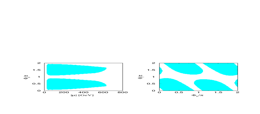
In this scenario, we expect that some cancellations among the CP phases are needed to suppress the electron EDM. Of course, the degree of the cancellations depends on the values of the real SUSY parameters, especially the higgsino mass parameter . The reason why we take a large of 700 GeV is to allow a relatively large region for the CP phases and while scanning the phase from 0 to . The fact that the allowed region of two phases increases with has been pointed out in the work by Brhlik, Good and Kane [6].
We display in Figure 2 (a) the allowed range of versus at 95% confidence level in the scenario for other phases sampled randomly within their allowed ranges. The overall trend clearly shows that for larger values of it is much easier to satisfy the electron EDM limits and any value of larger than 650 GeV allows the full range of . Figure 2(b) shows the allowed region at 95% confidence level for the phases and in the scenario with GeV. Note that near the region for the phase can take any value. In our next analysis on the correlated associated production and decay of neutralinos, which are mainly related with the CP phases and but not with the phase , Figure 2(b) will serve as the basic platform for all the contour plots for production cross sections, total cross sections of the correlated process, the branching ratios, several CP–even and CP–odd observables and an interesting CP–odd (T–odd) triple momentum product of the initial electron momentum and two lepton momenta from the leptonic decays of the neutralinos.
IV Associated Production of Neutralinos
A Production helicity amplitudes
Although we are mainly interested in one production process , we discuss in this section the associated production of every combination of neutralino–pair [–4] on a general footing. Note that the chirality mixing of scalar electrons are determined by the very small electron Yukawa coupling proportional to the electron mass much smaller than the collider c.m. energy (500 GeV) under consideration by a factor of about 106. Therefore, the selectron left–right chirality mixing can be safely neglected in the associated production of neutralinos so that the trilinear term does not play any role in the high energy process unlike the case for the electron EDM. In this approximation, the production process is generated by the five mechanisms shown in Fig. 3: -channel exchange, -channel exchanges, and -channel exchanges. The transition matrix element, after an appropriate Fierz transformation of the exchange amplitudes
| (33) |
can be expressed in terms of four generalized bilinear charges, classified according to the chiralities of the associated electron and neutralino currents
| (34) | |||||
| (35) | |||||
| (36) | |||||
| (37) |
with –, –, and –channel propagators and the couplings , and :
| (38) | |||
| (39) | |||
| (40) |
with , and . And, the combinations , and of the neutralino diagonalization matrix elements
| (41) | |||
| (42) | |||
| (43) |
satisfy the hermiticity relations reflecting the CP relations
| (44) |
so that, if the –boson width is neglected in the –boson propagator , the bilinear charges also satisfy the same relations with and interchanged in the propagators. The relation is very useful in classifying CP–even and CP–odd observables in the following.
Figure 3: Five mechanisms contributing to the production of neutralino pairs in annihilation, .
All physical observables (which can be constructed and measured through
the production process) are expressed in a simple form by 16 so–called
quartic charges [24] which contain important dynamical properties of
the process and are expressed in terms of the bilinear charges
. These quartic charges are classified according to
their transformation properties under parity as follows:
(a) Eight P–even terms:
| (45) | |||
| (46) | |||
| (47) | |||
| (48) | |||
| (49) | |||
| (50) | |||
| (51) | |||
| (52) |
(b) Eight P–odd terms:
| (53) | |||
| (54) | |||
| (55) | |||
| (56) | |||
| (57) | |||
| (58) | |||
| (59) | |||
| (60) |
We note that these 16 quartic charges comprise the most complete set for any fermion–pair production process in collisions when the electron mass is neglected. On the other hand, the quartic charges defined by an imaginary part of the bilinear–charge correlations might be nonvanishing only when there are complex CP–violating couplings or/and CP–preserving phases like recattering phases or finite widths of the intermediate particles. So, if there are no CP–preserving phases, non–vanishing values of these quartic charges signal CP violation in the given process.
Defining the production angle with respect to the electron flight direction by , the helicity amplitudes can be determined from Eq. (33). Electron and positron helicities are opposite to each other in all exchange amplitudes, but the and helicities are less correlated due to the non–zero masses of the particles; amplitudes with equal neutralino helicities must vanish only for asymptotic energies. Denoting the electron helicity by the first index, the and helicities by the remaining two indices, the helicity amplitudes are given by
| (61) | |||
| (62) | |||
| (63) | |||
| (64) |
for the right–handed electron beam, and
| (65) | |||
| (66) | |||
| (67) | |||
| (68) |
for the left–handed electron beam, where with and . The explicit form of the production helicity amplitudes have been obtained by the so–called 2–component spinor technique of Ref. [25]. If the arguments are not specified, the notation stands for in the following.
B Neutralino mass spectrum and production cross section
1 Neutralino masses
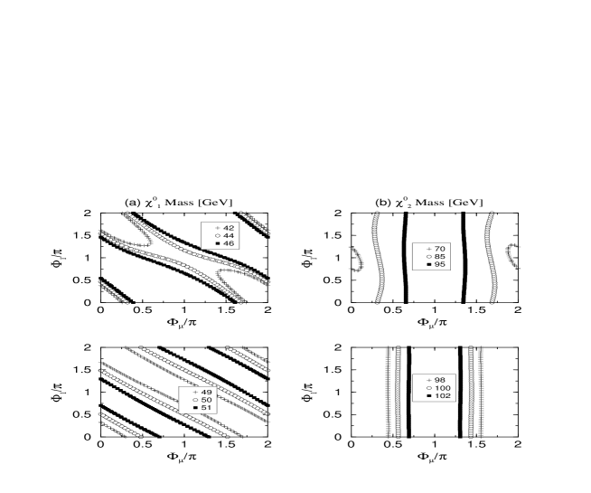
Before investigating various dynamical distributions in the neutralino processes, it will be worthwhile to see the dependence of the neutralino masses and of the gaugino composition of the two light neutralino states on the CP phases in two scenarios and . Figure 4 shows the mass spectrum of the neutralinos on the plane of the CP phases and in the two scenarios; (a) (upper figures) and (b) (lower figures). Except for the region around in , the second–lightest neutralino mass is (almost) independent of in both and , while the lightest neutralino mass exhibits a very strongly correlated dependence on the CP phases. Note that becomes maximal at non–trivial values of and in with GeV. This feature leads immediately to the conclusion that is strongly affected by a small value of , while is essentially determined by the SU(2) gaugino mass . Combined with the electron EDM constraints shown as the shadowed region in Fig. 1, the mass becomes smaller as the CP phases and approach the off–diagonal line on the plane, which implies that the mass is a function of the sum of two CP phase to a very good approximation.
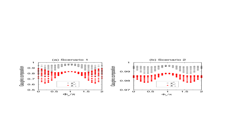
Since the phase is related with the gaugino part while the phase with the higgsino part, the size of their contributions will be strongly dependent on the size of the gaugino (or higgsino) compositions of the neutralino states. So, we present in Figure 5 the gaugino compositions and of the lightest and second–lightest neutralinos and defined by
| (69) | |||
| (70) |
with respect to the phase while the phase is scanned over its full allowed range in the scenarios (a) and (b) . As expected, has larger gaugino composition than . Certainly, the gaugino composition in the scenario is almost 100% due to the large value of GeV compared to the gaugino masses and . For around , the gaugino compositions are almost insensitive to the phase . On the contrary, in the region of , the gaugino compositions are very sensitive to the phase . This feature is partially responsible for the fact that in the scenario , the neutralino masses are strongly dependent on the phase around .
2 Production cross section
One of the important distributions in the production process is the differential cross section averaged over the initial beam polarizations. This unpolarized differential production cross section is given by taking the average/sum over the initial/final helicities:
| (71) |
Carrying out the sum, one finds the following expression for the differential cross section in terms of the scattering angle and the quartic charges:
| (73) | |||||
Figure 6 shows the dependence of the production cross section on the scattering angle and on the CP phases in the scenario (a) and (b) for a given c.m. energy of 500 GeV. Several interesting features are noted:
-
Two distributions are forward-backward symmetric, which is due to the Majorana property of the neutralinos. This symmetry property can be traced back to the fact that the quartic charge is directly proportional to and the quartic charges are forward–backward symmetric due to the Majorana relation where stands for the electron chirality.
-
The cross sections in the scenario with small selectron masses are much larger in size that those in the scenario with very large selectron masses. This reflects the fact that the – and –channel selectron exchanges become dominant for small selectron masses so that the production cross sections are very much enhanced. One additional crucial reason for the enhancement is that two neutralino states are more gaugino–dominated in the scenario than in the scenario .
-
The cross sections due to the selectron exchanges are smaller in the forward–backward directions in contradiction with a naive expectation of forward-backward peaking phenomena due to – and/or –exchanges. The reason is that while the contribution is suppressed in the scenario it is comparable in size with the other contributions with opposite sign in the scenario . Therefore, in the forward and backward directions, there exist a large cancellation among separate contributions.
-
The production cross section is more sensitive to the CP phases in the scenario than in the scenario ; the absolute production rate is much larger and the change due to different phases is larger as well in the scenario . So, we can expect in the scenario that the cross section itself can allow for a good determination of the phases.
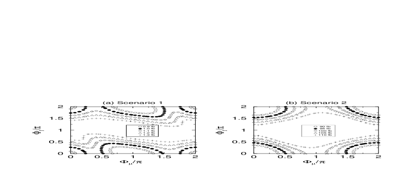
On the other hand the contours of the total production cross sections for the associated production of neutralinos are displayed in Figure 7 on the plane of the phases for a given energy of 500 GeV and for two SUSY parameter sets of the scenarios (a) and (b) . The total production cross section is of the order of 1 fb in the scenario while it is of the order of 100 fb in the scenario . In the scenario , the cross section is large when the phase is around and the phase is around and . However, the cross section in the scenario increases as the phases and approach the central point along the diagonal as well as off–diagonal lines.
C Initial beam polarizations
1 Spin–spin correlations
At future colliders, it is expected that highly longitudinally polarized electron and/or positron beams are available. On the other hand, it is uncertain if high transversely polarized beams can be easily obtained unlike conventional circular colliders. Nevertheless, it is interesting to investigate the effects of the longitudinal and transverse polarizations of the initial beams for the determinations of the fundamental SUSY parameters. So, in this section, we introduce a general formalism to describe the polarization effects of the initial beams for any production process. Here, the extremely small electron and positron masses ( ) compared to the collision energy of the order of 100 GeV allows us to have a very much simplified formalism. Neglecting the electron mass renders the positron helicity opposite to the electron helicity in any theory preserving electronic chirality as shown before. Let us consider the neutralino–pair production process , which is nothing but the process under consideration. For the sake of convenience we introduce a bracket notation for all the helicity amplitudes which is guaranteed by the electronic chirality invariance and which enables us to obtain a simple form of the polarization–weighted squared matrix element as
| (77) | |||||
where and denote the degree of longitudinal and transverse polarization of the electron (positron), and the direction of each transverse polarization with respect to a given reference plane, for which the scattering plane is chosen in most cases. The pictorial description of the azimuthal angles is given in Figure 8. We emphasize that the formalism can be applied to any collision process preserving electronic chirality with an apporiate choice of reference frame to define the azimuthal angle parameters and .
Figure 8: Configuration of transverse polarization vectors in the center–of–mass frame. The azimuthal angles and denote the orientation of the polarization vectors with respect to a reference plane, for which the scattering plane is chosen.
The longitudinal and transverse polarizations and the azimuthal angles for the transverse polarizations are related under CP transformations as follows:
| (78) | |||||
| (79) | |||||
| (80) |
while the production helicity amplitudes are related under CP transformations as:
| (81) |
where the subscript means for the production of a particle and an anti–particle according to our spinor conventions. Denoting as the CP-conjugate polarization–correlated distribution of , one can construct a CP–even distribution and a CP-odd distribution . If no CP–preserving phases are involved or any of them are negligible in a given process, one can find that the CP–odd distribution is proportional to the last term of the distribution in Eq. (77), while the CP–even distribution is composed of the other three terms.
2 Two additional CP–even observables
Neglecting the –boson width (), which is very small compared to the collision energies under consideration, the distribution (77) provides us with three CP-even observables; one of them is the unpolarized part which has been discussed before and the other two terms can be extracted by taking an appropriate polarization correlation. Longitudinal polarization yield a differential left-right (LR) asymmetry
| (82) |
with the normalization corresponding to the unpolarized part
| (83) |
The LR asymmetry can readily be expressed in terms of the quartic charges,
| (85) | |||||
with, correspondingly, the expression for the normalization
| (87) | |||||
It will be straightforward to extract the integrated left–right asymmetry experimentally with the expectation that highly longitudinally polarized beams are available at future linear colliders. Certainly, the extraction efficiency depends linearly on the degree of electron and positron polarization obtainable at the collisions.
The other transverse–polarization dependent term can be separated by allowing transverse polarization and setting longitudinal polarization to zero. Note that the transverse term is dependent on the sum of two azimuthal angles and , which must be sorted out by using a weight function . This projection requires that the scattering plane is experimentally determined event by event. First of all, the neutralino masses and are expected to be measured with good precision through identifying the minimal and maximal values for the lepton invariant mass in the leptonic decay . The determined masses and the four–momentum of two final leptons enable us to determine only the polar angle between the flight direction and the flight direction in the laboratory frame. Certainly, if the c.m. energy is so large that neutralino masses are negligible, the neutralino direction can be identified with the direction of the two–lepton momentum. However, for a moderate c.m. energy, it is not possible to completely determine the scattering angle. Nevertheless, this distribution will affect the final two–lepton distribution partially so that it is not useless to investigate the dependence of the observable on the SUSY parameters. The CP–even observable obtained through the angular projection procedure is given by
| (88) |
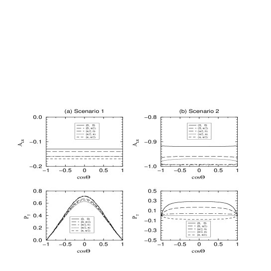
The upper figures in Figure 9 exhibit the LR asymmetries and the lower ones the CP–even observables for the production of the associated pair and as a function of the scattering angle at a c.m. energy of 500 GeV in the scenarios (a) and (b) for five combinations of the CP phases . We note that these two observables are also more sensitive to the CP phases in the scenario than in the scenario . However, the sensitivity of the LR asymmetry to the CP phases is not strong, so that the asymmetries are not very useful in determining the phases. On the other hand, as discussed before, the CP–even observable, which is more sensitive to the phases, is not easy to extract experimentally. Therefore, we may conclude that these two observables are not so powerful in determining the phases in both scenarios, while satisfying the constraints from the electron EDM measurements.
3 One CP–odd observable
CP violation arises in the existence of nontrivial complex couplings in the Lagrangian. In the associated production of the neutralinos CP violation is reflected in the complex production amplitudes. First of all, we find that in every diagonal production of neutralinos the production amplitude is purely real with the –boson width neglected, and it leads to no CP-violation.
Like the CP-even observable , the only T-odd term , which is CP-odd in the absence of any CP-even rescattering phases like the –boson width, can be separated by allowing transverse polarization and setting longitudinal polarization to zero with as a projection angular function. As a result, one can obtain a CP-odd observable as
| (89) |
One can check with the definition of the quartic charge that if the –boson width is neglected, the T-odd observable may be non-zero only for since for all the bilinear charges are real.
In CP–noninvariant theories the quartic charge , which is non–vanishing for , can be expressed in terms of two Jarlskog-type CP-odd rephasing invariants [26] of the diagonalization matrix . In order to elaborate on this point further, we present the explicit form of the quartic charge; assuming a real -boson propagator the quartic charge is given by
| (90) |
Two combinations of the couplings, and , are rephase-invariant. Using the expressions for , and , we can rewrite the two combinations as
| (91) | |||
| (92) |
where the primed matrix elements and are related with the diagonalization matrix elements and through
| (93) |
From the expressions (37) and (38), we can draw the following consequences:
-
Both and require the existence of gaugino and higgsino components and a different magnitude of two higgsino components of the and states. This latter requirement means that should be different from unity.
-
The distribution is forward–backward asymmetric, because the angular dependence is determined by the difference .
-
Due to the large suppression in the – and –channel selectron exchanges, the T–odd asymmetry is very small in the scenario . Moreover, the asymmetry is very small in the scenario as well. This suppression is because the observable requires a sizable mixing between gaugino and higgsino states, but the mixing is very small due to the large value of compared to the gaugino masses and .
As a whole, these features lead to the conclusion that the T–odd observable is not useful in measuring the CP phases directly in both scenarios and suggested by the analysis for the electron EDM constraints.
4 Neutralino polarization vector
Neutralinos are spin–1/2 particles and their polarization can be measured through their decays. Before we investigate the possible neutralino decays in detail, in this section we study chargino polarization directly in the production process with unpolarized initial beams. The polarization vector of the produced neutralino is defined in the rest frame in which the axis is in the flight direction of , rotated counter–clockwise in the production plane, and of the decaying neutralino . Accordingly, the component denotes the component parallel to the flight direction in the c.m. frame, the transverse component in the production plane, and the component normal to the production plane. These three polarization components can be expressed by helicity amplitudes in the following way:
| (94) | |||
| (95) | |||
| (96) |
The longitudinal, transverse and normal components of the polarization vector can be easily obtained from the production helicity amplitudes. Expressed in terms of the quartic charges, they read:
| (97) | |||
| (98) | |||
| (99) | |||
| (100) |
where the reduced masses . The longitudinal and transverse components are P–odd and CP–even, and the normal component is P–even and CP–odd.
The normal polarization component can only be generated by complex production amplitudes. Non–zero phases are present in the fundamental SUSY parameters if CP is broken in the supersymmetric interaction. Also the non–zero width of the boson and loop corrections generate non–trivial phases; however, the width effect is negligible for high energies as mentioned before, and the effects due to radiative corrections are small as well. So, the normal component is effectively generated by the complex SUSY couplings. As the selectron–exchange contributions can be ignored in the scenario , the CP–odd quartic charge simplifies to
| (101) |
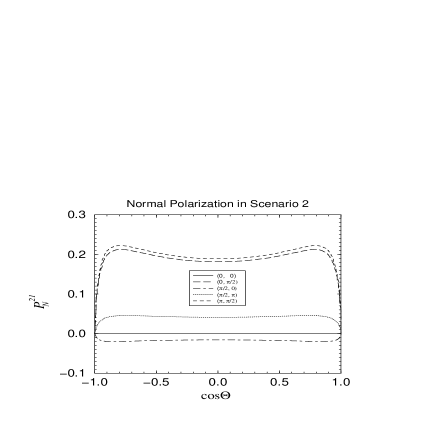
Since the presently measured value of is [27] very close to , the quartic charge is extremely suppressed in the scenario . However, in the scenario , the quartic charge can be relatively large without such a big suppression as shown in Figure 10. In this case, the normal polarization is of the order of 10 %, which is really sizable for non–trivial CP phases and very sensitive to the CP phases . So, it is expected to give stringent constraints on the phases . These strong constraints will be explicitly demonstrated in the following.
V Neutralino Decays
A Decay density matrix
Assuming the lightest neutralino to be the lightest supersymmetric particle (LSP), several mechanisms contribute to the leptonic decays of the neutralino ():
In particular, the leptonic three body decay of the second lightest neutralino, , is known to be very important because the end point of the lepton invariant mass distribution gives us direct information on the mass difference between and , which provides us with a stringent constraints on MSSM parameters.
Although we will take into account only electrons and muons for the final state leptons, let us make some comments on the other possible leptonic decay of the second lightest neutralino, [21]. Since is the heaviest lepton with a much larger mass ( GeV) than the other leptons and it couples with Higgs bosons with the strength proportional to , the branching fraction of this leptonic decay mode can be very different depending on the value of and the Higgs mass spectrum. Actually, the mode is known to be very much enhanced due to the Higgs exchanges at large [21]. Furthermore, the polarization of can be observed through the decay distributions, which strongly depend on the parent polarization [28].
Due to the missing tau neutrinos, one would not be able to measure the invariant mass of two tau leptons experimentally. Nevertheless the polarization or the invariant mass of the two jets might be seen in future collider experiments. We note that in or decays, the final vector meson carries a substantial part of the parent momentum, therefore the smearing of the distribution is less severe than for decays into , and . Let us give several comments on the tau decay mode. First of all, for , the effects of the Yukawa couplings and slepton left–right mixing could be very important for large . Their leading contribution flips the chirality of the lepton [29]. Secondly, for the three body decays, studying the correlation of two tau decay distributions would reveal the helicity flipping and conserving contributions separately. Thirdly, staus could be lighter than the other sleptons for various reseaons. The running of stau soft SUSY breaking masses from the Planck scale and stau left–right mixing could enhance decays into . Experimental consequences of such scenarios have recently been widely discussed. Also models with lighter third generation sparticles have been naturally constructed without causing the flavor changing neutral current problem. The three body decay branching ratio and the decay distribution might be different from those for leptons in the first two generations. Since the study of the decay in addition to the other leptonic modes could be an important handle to identify such models, we plan to present a detailed investigation about all these interesting features in the near future.
Figure 11: Neutralino decay mechanisms; the exchange of the neutral Higgs boson is neglected because of the tiny electron Yukawa coupling.
The diagrams contributing to the process with , are shown in Fig. 11 for the decay into lepton pairs. Here, the exchange of the neutral Higgs boson [replacing the boson] are neglected since the couplings to the light first and second generation SM leptons are very small. In this case, all the components of the decay matrix elements are of the left/right currentcurrent form which, after a simple Fierz transformation, may be written for lepton final states as
| (102) |
with the generalized bilinear charges for the decay amplitudes:
| (103) | |||||
| (104) | |||||
| (105) | |||||
| (106) |
where the chiralities stand for the chiralities and and channel propagators and the couplings and are given in the section for the production helicity amplitudes. The Mandelstam variables are defined in terms of the 4-momenta of and , respectively, as
| (107) |
The decay distribution of a neutralino with polarization vector is
| (112) | |||||
where is the spin 4–vector and . Here, the quartic charges and for the neutralino decays are defined by
| (113) | |||
| (114) | |||
| (115) | |||
| (116) | |||
| (117) | |||
| (118) | |||
| (119) |
If needed, the polarization of the final neutralino can be incorporated in a straightforward manner although the decay distribution will be more complicated in its form.
For the subsequent discussion of the angular correlations between two neutralinos, it is convenient to determine the decay spin density matrix . In general, the decay amplitude for a spin–1/2 particle and its complex conjugate can be expressed as
| (120) |
with the general spinor structure and . Then we use the general formalism to calculate the decay density matrix involving a particle with four momentum and mass by introducing three space-like four vectors () which together with form an orthonormal set:
| (121) |
where and with . A convenient choice for the explicit form of is in a coordinate system where the direction of the three–momentum of the particle is lying on the - plane:
| (122) |
Then in this reference frame, describe transverse, normal and longitudinal polarization of the particle.
With the four–dimensional basis of normal four–vectors , we can derive the so–called Bouchiat–Michel formula [30]
| (123) |
which can be used to compute the squared, normalized decay density matrix
| (124) |
where () are the Pauli matrices and the four kinematic functions and ()
| (126) | |||||
| (129) | |||||
with () three vectors forming the polarization basis for the decaying spin–1/2 particle.
B Branching ratios
Since the reconstruction of the neutralino-pair production depends on the efficient use of the neutralino decay modes, it is necessary to estimate the branching fraction of each decay mode. Since we assume that the lightest neutralino is the LSP and we are interested only in the decay of the second–lightest neutralino , we can classify the decay modes as follows:
| (130) | |||
| (131) |
Besides, if the mass is smaller than the neutralino mass , the lightest chargino can enter the neutralino decay chain via . Concerning the neutralino decays, there are several aspects worthwhile to be commented on:
-
For the first and second generation fermions, the Higgs–exchange diagrams are suppressed unless is very large.
-
The experimental bounds on the Higgs particles are very stringent so that the two–body decays and are expected to be not available or at least strongly suppressed.
-
The lightest chargino and the second–lightest neutralinos are almost degenerate in the gaugino–dominated parameter space so that the charged decays such as will be highly suppressed.
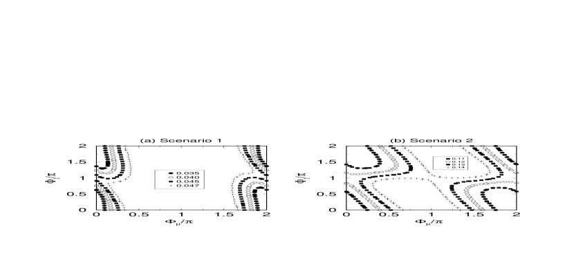
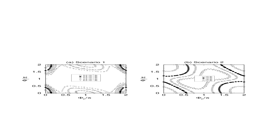
Nevertheless, we calculate the leptonic branching fractions fully incorporating all the possible decay modes of the neutralino while neglecting the Higgs-exchange contributions for a small . In our numerical analysis, we assume 200 GeV for a common soft–breaking slepton mass and 500 GeV for a common soft–breaking squrk mass in the scenario while we take 10 TeV for all the soft–breaking sfermion masses in the scenario . Figure 12 shows for or in the scenarios (a) and (b) . We find that the branching fractions are very sensitive to only around in the scenario , while it depends very strongly on and on (almost) the whole space of the phases in the scenario . Furthermore, the branching fraction is very much enhanced in the scenario because the slepton–exchange contributions due to mainly the gaugino components of the neutralinos become dominant due to the small slepton masses while the large value of suppressing the higgsino components. Consequently, the branching ratio of the leptonic decay of the second lightest neutralino is very sensitive to the values of the underlying parameters, in particular, the CP phases.
VI Spin and Angular correlations
A Correlations between production and decay
In this section, we provide a general formalism to describe the spin correlations between production and decay for the process followed by the sequential leptonic decay . For the sake of convenience, we do not consider the initial beam polarization, which can however be easily implemented. Formally, the spin–correlated distribution is obtained by taking the following sum over the helicity indices of the intermediate neutralino state by folding the decay density matrix and the production matrix formed with production helicity amplitudes:
| (132) |
where the functions of the scattering angle are given in terms of the production helcity amplitudes by
| (133) | |||||
| (134) | |||||
| (135) | |||||
| (136) |
Notice that the above combinations are directly related with the polarization vector of the neutralino as follows
| (137) |
Combining production and decay, we obtain the fully–correlated 6-fold differential cross section
| (138) |
where
| (139) |
with the phase space volume element . The angular variable is the polar angle of the in the rest frame with respect to the original flight direction in the laboratory frame, and the corresponding azimuthal angle with respect to the production plane, and is the relative azimuthal angle of along the direction with respect to the production plane. On the other hand, the opening angle between the and is fixed once the lepton energies are known. The pictorial description of the kinematical variables for the decay is presented in Fig. 13. The dimensionless parameters and denote the lepton energy fractions
| (140) |
with respect to the neutralino mass divided by a factor of two. The kinematically–allowed range for the variables is determined by the kinematic conditions
| (141) | |||
| (142) | |||
| (143) |
where , and the masses of the final–state leptons are neglected.
Figure 13: Configuration of momenta in the c.m. frame for the associated production of neutralinos and in the rest frame of the decaying neutralino .
B Total cross section of the correlated process
The total cross section for the correlated process is given by integrating the differential cross section (138) over the full range of the 6–dimensional phase space. More simply, the cross section is given as the multiplication of the integrated production cross section and the branching fraction because the correlation effects are washed out after integration over the phase space volume.
The total cross section is displayed in Figure 14 as the contour plots on the plane of two CP phases in two scenarios (a) and (b) . First of all, we note that the total cross section in the scenario is very small. By definition, the scenario has extremely large selectron masses so that only the –exchange diagram involving only the higgsino composition of the neutralinos contributes. However, the higgsino composition of the neutralinos is at most 40% and in most cases 20% for while it is at most 20% and in most cases 10% for . Therefore, it is naturally expected to have a strongly–suppressed cross section in the scenario. On the other hand, the total cross section is very much enhanced in the scenario , mainly due to large gaugino composition and small selectron masses which contribute to the cross section through the – and –channel exchanges. So, we can conclude that it is possible to have a relatively large cross section if the higgsino composition of the neutralinos is large or the slepton masses are small [5].
Quantitatively the scenario will present a few events of the neutralino process for a integrated luminosity of the order of 100 fb-1 while the scenario give a few thousand events for the same integrated luminosity. So, a good precision measurement of the relevant SUSY parameters might be performed in the scenario at future high luminosity collider experiments such as TESLA, while it might be difficult in the scenario . As can be read from the figures, the cross section increases as the phase approaches in both scenarios. However, the dependence of the cross section on the phase is very different in two scenarios. In the scenario , the cross section increases monotonically as approaches , but it becomes maximal at a non-trivial value of between () and in the scenario .
Compared with the dependence of the neutralino masses on the CP phases displayed in Figure 4, the cross section can be larger for larger neutralino masses and vice versa for quite large region of the CP phases. This implies that within the range allowed in the scenarios the signals with larger masses can have more possibility of being detected while those with smaller masses may escape detection. In this sense, future high luminosity experiments can give constraints on the CP phases simply by putting the upper limits on the event rates.
C Dilepton invariant mass distributions
The invariant mass of two final–state leptons , which is nothing but the square root of the Mandelstam variable, ,
| (144) |
is a Lorentz–invariant kinematical variable so that it is easy to reconstruct by measuring the energies of two final–state leptons [31]. Furthermore, the distribution for the invariant mass is independent of the specific production process for the decaying neutralino. This factorization is due to the fact that the invariant mass does not involve any angular variables describing the decays so that the polarization of the decaying neutralino is not effective.
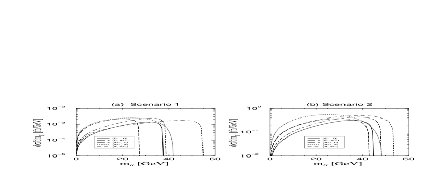
Figure 15 shows the two–lepton invariant mass distribution in the scenarios (a) and (b) . This distribution must reflect the two–lepton invariant mass distribution of the neutralino decay itself multiplied by the total production cross section . As shown before, the leptonic branching ratio is very sensitive to the values of the underlying SUSY parameters. We find that the distribution of the invariant mass of the final–state two leptons is sensitive to the the CP phases as well. First of all, the end point of the maximal invariant mass is strongly dependent on the CP phases so that after all the real parameters are determined, the measurement of the end point will provide us with a very good handle to determine the CP phases. As one can notice from Figure 15, the sensitivity is larger in the scenario with a small parameter, which is more comparable to the value of than in the scenario . It clearly implies that the effect of the CP phases is enhanced for comparable gaugino and higgsino parameters.
In passing, we note that since it is independent of the production mechanism, the lepton invariant mass distribution can be an important tool for studying supersymmetric models even at hadron colliders because of its clean signature. This point has been in detail explored by Nojiri and Yamada [31] by investigating the parameter dependence of the distribution of the three body decay at the CERN LHC.
D Lepton angular distribution in the laboratory frame
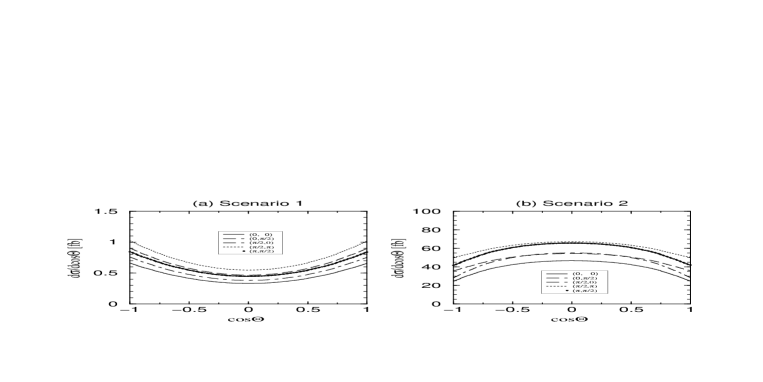
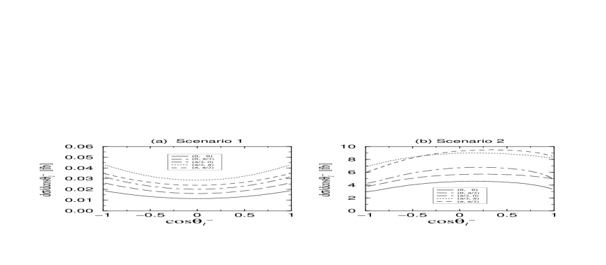
In this section, we give numerical results for the angular distributions of with respect to the electron beam axis computed with complete spin correlations between production and decay. Unlike the invariant mass distribution, this lepton angular distribution is crucially dependent on the production–decay spin correlations. Moortgat–Pick and Fraas [14] have found in their detailed study that the effect of the spin correlations for the lepton angular distribution amounts up to 20% for lower energies and the shape of the lepton angular distribution is very sensitive to the mixing in the gaugino sector and to the value of the slepton mass. These points can be confirmed by comparing two results displayed in Figure 16. In the scenario (left figure) with large selectron masses, the lepton angular distribution is forward–backward symmetric and larger in the forward–backward direction. On the other hand, in the scenario the angular distribution is forward–backward asymmetric, maximal near but suppressed in the forward–backward directions. Furthermore, the size of the lepton angular distribution and the forward–backward asymmetry depends rather strongly on the CP phases.
E Triple momentum product
So far, we concentrate mainly on the CP–even production–decay correlated observables which depend on the CP phases only indirectly. However, the initial electron momentum and two easily–reconstructible final–state leptons allows us to construct a T–odd observable
| (145) |
with . This T–observable [19] can be finite if there exist non–vanishing CP–violating or CP–preserving complex phases in the amplitude for the correlated process. If we neglect the heavy particle widths, the T–odd observable can be utilized to directly measure the CP phases or to constrain them.
Due to the general property of the T–odd observable, we know that it should be given a linear combination of the CP–odd quartic charges and . Note that in the scenario with large slepton masses, both of them are proportional to a small suppression factor as noticed in Eq. (42). Therefore, the T–odd observable as well as the electron EDM can not give any significant constraints on the CP phases in the scenario . On the other hand, since the slepton exchanges give a large contribution in the scenario , there might be a relatively large value of the T– (CP–)odd observable for no–trivial phases. Furthermore, since the fundamental structure of the electron EDM determined by the CP phases will be very different from that of the T–odd observable, two CP–odd quantities will play a complementary role in constraining the CP phases. In order to make a concrete comparison of them, we explore the exclusion region by the T–odd observable on the CP phases in the scenario . Since we cannot estimate the precise systematic uncertainties mainly related with the detection quality, we neglect the systematic uncertainties but take into account only the statistical errors. In this case, the boundaries of the excluded region of the CP phases and at the – level for a given integrated luminosity satisfy the relation
| (146) |
where over the total phase space volume . In determining the exclusion area we take into account two possible combinations of two final–state leptons; and , which is responsible for the factor 2 in the denominator.
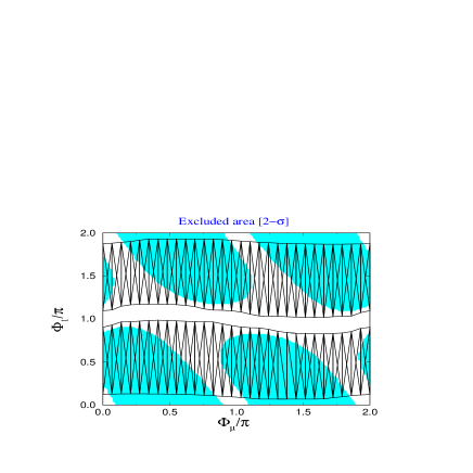
Figure 17 exhibits the excluded area of the CP phases by the electron EDM measurements at 95% confidence level (shaded region) and by the T–odd observable (hatched region) at a 2– level with an integrated luminosity of 200 fb-1. One can clearly notice their complementarity role played by two independent CP–odd quantities. The T–odd observable enables us to exclude all the range of for most values of except for . In addition, they are complementary in the sense that the electron EDM is an indirect physical quantity determined at a very low energy, which does not need to observe SUSY particles but the T–odd observable is a direct observable to measure the SUSY CP phases exclusively, which however requires producing neutralinos directly. So, we conclude that through our investigations the T–odd observable can be a very efficient and complementary quantity in constraining or determining the CP phases if the lightest and second lightest neutralinos are pair–produced and unless the sleptons are too heavy.
VII Conclusions
In this paper, we have investigated the associated production of neutralinos accompanied by the neutralino leptonic decay , taking into account initial beam polarization and production-decay spin correlations in the minimal supersymmetric standard model with general CP phases but without generational mixing in the slepton sector. The stringent constraints by the electron EDM on the CP phases have been also included in the discussion of the effects of the CP phases.
First of all, we have described possible flavor–preserving – selectron, chargino and neutralino – mixings in the MSSM with general CP phases without generational mixing and applied them to the evaluation of the electron EDM to investigate its dependence on the phases. As a result, we have identified two typical scenarios; one has large selectron masses of the order of 10 TeV and the other relatively light selectron masses of 200 GeV and a large higgisino mass parameter. The first scenario allows the full range for the CP phases and relevant to the neutralino process while the second scenario allows a finite space for the CP phases. Employing the allowed space as the platform for further investigations of the neutralino processes, we have obtained several interesting results, which can be summarized as follows:
-
The production cross section and the branching fractions of the leptonic neutralino decays are very sensitive to the CP phases. As a result, the total cross section is very sensitive to the CP phases.
-
If the electron/positron masses are neglected, the initial longitudinal and transverse polarizations of the initial electron and positron beams lead to three CP–even distributions and one CP–odd distribution, which can be studied independently of the details of the neutralino decays. While they are sensitive to the real SUSY parameters, those observables, especially, the T– (CP–)odd observable is (almost) insensitive to the CP phases in both scenarios.
-
The production–decay spin correlations lead to several CP–even observables among them we have studied the two–lepton invariant mass distribution, the lepton angular distribution, and one interesting T–odd (CP–odd) triple product of the initial electron momentum and two final lepton momenta. On the whole, we have found that the distributions are sensitive to the CP phases in the scenario with relatively light selectrons and large gaugino compositions of the neutralinos.
-
We have presented the exclusion region of the CP phases and by the T–odd (CP–odd) observable with the assumed integrated luminosity of 200 fb-1 at 2- level. In comparison with the constraints from the electron EDM measurements, the constraints from the T–odd observable is complementary in that it constrains very strongly the phase .
To conclude, the associated production of neutralinos followed by the leptonic decays is expected to be one of the cleanest SUSY processes to allow for a detailed investigation of the physics due to the CP phases in the MSSM. Therefore, if the neutralinos are produced at future colliders, the colliders will make it possible to measure or constrain the SUSY parameters and CP phases and so provide a complementary check for the existence of CP violation in the MSSM in the neutralino sector.
Acknowledgments
The authors are grateful to Monoranjan Guchait for valuable comments. S.Y.C. would like to thank Manuel Drees for useful suggestions and helpful discussions for the present work and also thank Francis Halzen and the Physics Department, University of Wisconsin–Madison where part of the work has been carried out. The work of H.S.S and W.Y.S was supported in part by the Korea Science and Engineering Foundation (KOSEF) through the KOSEF–DFG large collaboration project, Project No. 96–0702–01-01-2, and in part by the Center for Theoretical Physics. S.Y.C wishes to acknowledge the financial support of 1997-sughak program of Korean Reseach Foundation.
REFERENCES
- [1] For reviews, see H. Nilles, Phys. Rep. 110, 1 (1984); H.E. Haber and G.L. Kane, Phys. Rep. 117, 75 (1985); S. Martin, in Perspectives on Supersymmetry, edited by G.L. Kane, (World Scientific, Singapore, 1998).
- [2] S. Dimopoulos and D. Sutter, Nucl. Phys. B 452 (1995) 496; H. Haber, Proceedings of the 5th International Conference on Supersymmetries in Physics (SUSY’97), May 1997, ed. M. Cvetić and P. Langacker, hep-ph/9709450.
- [3] A. Masiero and L. Silvetrini, in Perspectives on Supersymmetry, edited by G.L. Kane, (World Scientific, Singapore, 1998); J. Ellis, S. Ferrara and D.V. Nanopoulos, Phys. Lett. B114, 231 (1982); W. Buchmüller and D. Wyler, ibid. B121, 321 (1983); J. Polchinsky and M.B. Wise, ibid. B125, 393 (1983); J.M. Gerard et al., Nucl. Phys. B253, 93 (1985); P. Nath, Phys. Rev. Lett. 66, 2565 (1991); R. Garisto, Nucl. Phys. B419, 279 (1994).
- [4] M. Brhlik and G.L. Kane, Phys. Lett. B 437, 331 (1998); S.Y. Choi, J.S. Shim, H.S. Song and W.Y. Song, ibid. B 449, 207 (1999).
- [5] J. Ellis, J. Hagelin, D. Nanopoulos and M. Srednicki, Phys. Lett. 127B (1983) 233; V. Barger, R.W. Robinett, W.Y. Keung and R.J.N. Phillips, Phys. Lett. B131 (1983) 372; D. Dicuss, S. Nandi, W. Repko and X. Tata, Phys. Rev. Lett. 51 (1983) 1030; S. Dawson, E. Eichten and C. Quigg, Phys. Rev. D31 (1985) 1581; A. Bartl and H. Fraas and W. Majerotto, Z. Phys. C30 (1986) 441.
- [6] T. Ibrahim and P. Nath, Phys. Rev. D 57, 478 (1998); M. Brhlik, G.J. Good and G.L. Kane, ibid. D 59, 115004-1 (1999); S. Pokorski, J. Rosiek and C.A. Savoy, hep–ph/9906206.
- [7] Y. Kizukuri and N. Oshimo, Phys. Rev. D D45, 1806 (1992); 46, 3025 (1992).
- [8] S. Dimopoulos and G.F. Giudice, Phy. Lett. B 357, 573 (1995); A. Cohen, D.B. Kaplan and A.E. Nelson, ibid. B 388, 599 (1996); A. Pomarol and D. Tommasini, Nucl. Phys. B488, 3 (1996).
- [9] T. Falk and K.A. Olive, hep-ph/9806236; T. Falk, A. Ferstl and K.A. Olive, hep-ph/9806413; T. Falk and K.A. Olive, Phys. Lett. B 375, 196 (1996); T. Falk, K.A. Olive and M. Srednicki, ibid. B 354, 99 (1995).
- [10] A. Pilaftsis and C.E.M. Wagner, hep-ph/9902371; D.A. Demir, hep-ph/9901389; B. Grzadkowski, J.F. Gunion and J. Kalinowski, hep-ph/9902308.
- [11] G.C. Branco, G.C. Cho, Y. Kizukuri and N. Oshimo, Phys. Lett. B 337, 316 (1994); Nucl. Phys. B 449, 483 (1995); D.A. Demir, A. Masiero and O. Vives, Phys. Rev. Lett. 82, 2447 (1999); S.W. Baek and P. Ko, hep-ph/9812229 (to appear in Phys. Rev. Lett.).
- [12] Proceedings of the Workshop on Physics at LEP II, Report No. CERN-96-01, eds. G. Altarelli, T. Sjöstrand, and F. Zwirner.
- [13] For reviews, see for example E. Accomando et al., Physics Reports 299 (1998) 1 and references therein.
- [14] G. Moortgat–Pick and H. Fraas, Phys. Rev. D 59, 015016-1 (1998).
- [15] A. Bartl, H. Fraas, W. Majerotto, and B. Mösslacher, Z. Phys. C 55, 257 (1992); S.T. Petcov, Phys. Lett. B139, 421 (1984); S.M. Bilenky, E.C. Christova, and N.P. Nedelcheva, Bulg. J. Phys. 13, 283 (1986).
- [16] A. Leike, Int. J. Mod. Phys. A3 (1988) 2895; M.A. Diaz and S.F. King, Phys. Lett. B349 (1995) 105; B373 (1996) 100; J.L. Feng and M.J. Strassler, Phys. Rev. D51 (1995) 4461 and D55 (1997) 1326; G. Moortgat-Pick and H. Fraas, Report WUE-ITP-97-026 (hep-ph/9708481).
- [17] S.Y. Choi et al., Eur. Phys. J. C 7, 123 (1999); G. Moortgat–Pick and H. Fraas, Phys. Rev. D 59, 015016-1 (1998); hep–ph/9903220.
- [18] S. Ambrosanio and B. Mele, Phys. Rev. D 52, 3900 (1995).
- [19] Y. Kizukuri and N. Oshimo, Phys. Lett. B249, 449 (1990).
- [20] D. Chang, W.-Y. Keung and A. Pilaftsis, Phys. Rev. Lett. 82, 900 (1999).
- [21] H. Baer, C. Chen, M. Drees, F. Paige, and X. Tata, Phys. Rev. Lett. 79, 986 (1997); 80, 642(E) (1998); Phys. Rev. D 58, 975008 (1998); 59, 055014 (1999).
- [22] M. Acciarri et al., L3 Collaboration, Preprint Number CERN-EP-99-080, Jun 1999; P. Abreu et al., DELPHI Collaboration, Preprint number CERN-EP-99-077, Jun 1999 and references therein.
- [23] E.D. Commins, S.B. Ross, D. DeMille, and B.S. Regan, Phys. Rev. A 50, 2960 (1994); K. Abdullah et al., Phys. Rev. Lett. 65, 2347 (1990).
- [24] L.M. Sehgal and P.M. Zerwas, Nucl. Phys. B183, 417 (1981).
- [25] K. Hagiwara and D. Zeppenfeld, Nucl. Phys. B274, 1 (1986).
- [26] C. Jarlskog, Phys. Rev. Lett. 55, 1039 (1985); Z. Phys. C 29, 491 (1985).
- [27] Particle Data Group, Eur. Phys. J. C 3, 1 (1998).
- [28] Y.S. Tsai, Phys. Rev. D 4, 2821 (1971); T. Hagiwara, S.-Y. Pi, and A.I. Sanda, Ann. Phys. (N.Y.) 106, 134 (1977); A. Rougé, Z. Phys. C 48, 75 (1990); H. Kühn and F. Wagner, Nucl. Phys. B236, 16 (1984); B.K. Bullock, K. Hagiwara, and A.D. Martin, Phys. Rev. Lett. 67, 3055 (1991); Phys. Lett. B273, 501 (1991); Nucl. Phys. B395, 499 (1993).
- [29] M.M. Nojiri, Phys. Rev. D 51, 6281 (1995); M.M. Nojiri, K. Fujii, and T. Tsukamoto, Phys. Rev. D 54, 6756 (1996).
- [30] C. Bouchiat and L. Michel, Nucl. Phys. 5, 416 (1958); L. Michel, Suppl. Nuovo Cim. 14, 95 (1959); S.Y. Choi, Taeyeon Lee, H.S. Song, Phys. Rev. D 40, 2477 (1989).
- [31] M.M. Nojiri and Y. Yamada, Phys. Rev. D 60, 015006-1 (1999).