Practical Algebraic Renormalization

Pietro Antonio Grassi^(a) , Tobias Hurth^(a) and Matthias Steinhauser^(b)
(a) Max-Planck-Institut für Physik,
Werner-Heisenberg-Institut, D-80805 Munich, Germany
(b) Institut für Theoretische Physik,
Universität Bern, CH-3012 Bern, Switzerland
Abstract A practical approach is presented which allows the use of a non-invariant regularization scheme for the computation of quantum corrections in perturbative quantum field theory. The theoretical control of algebraic renormalization over non-invariant counterterms is translated into a practical computational method. We provide a detailed introduction into the handling of the Slavnov-Taylor and Ward-Takahashi identities in the Standard Model both in the conventional and the background gauge. Explicit examples for their practical derivation are presented. After a brief introduction into the Quantum Action Principle the conventional algebraic method which allows for the restoration of the functional identities is discussed. The main point of our approach is the optimization of this procedure which results in an enormous reduction of the calculational effort. The counterterms which have to be computed are universal in the sense that they are independent of the regularization scheme. The method is explicitly illustrated for two processes of phenomenological interest: QCD corrections to the decay of the Higgs boson into two photons and two-loop electroweak corrections to the process $B\rightarrow X_{s}\gamma$.

1 Introduction

A regularization method which respects all symmetries of the Standard Model (SM) [1] does not exist. The popular and powerful method of Dimensional Regularization [2] is at least an invariant scheme for QCD. In the electroweak sector, however, the coupling to chiral fermions introduces the well-known $\gamma_{5}$ problem. One also has to face additional technicalities due to evanescent operators in the effective field theory approach. It is well-known that in the framework of Dimensional Regularization only the ’t Hooft-Veltman-Breitenlohner-Maison scheme [3, 4] for $\gamma_{5}$ is shown to be consistent to all orders. The so-called naive dimensional scheme (with an anticommuting $\gamma_{5}$) does not reproduce the chiral anomaly and is not consistent to all orders. For specific examples it leads to correct results at the lowest orders in perturbation theory. Nevertheless, it seems desirable to have a powerful practical alternative even in the SM, at least for cross-checks, as suggested controversies in the past suggest (see, e.g., [5]). Moreover, the impressive experimental precision mainly reached at the electron positron colliders LEP and SLC and the proton anti-proton collider TEVATRON has made it mandatory to evaluate specific two- or even three-loop contributions to observables where the inconsistencies of the well-known “naive dimensional” scheme are unavoidable.

Going beyond the SM, it is well-known that Dimensional Regularization breaks the Ward identities of supersymmetry. However, one very often prefers to keep the dimensional scheme for the practical calculations, also beyond the SM, in order to take advantage of already well-developed computer tools [6]. Thus, one needs a practical procedure to restore the Ward identities of supersymmetry in the final step of the renormalization procedure.

From the principal point of view, the calculation of higher-loop contributions in perturbative quantum field theories is a well-understood issue. The axioms of relativistic quantum field theory, such as causality and Poincaré invariance, fix the matrix elements completely to all orders up to a limited number of free constants. They have to be determined by renormalization conditions. These free constants correspond to a renormalization ambiguity for coinciding points in the definition of time-ordered products of operator-valued distributions [7]. The main question is whether the renormalization ambiguity can be fixed in such a way that the time-ordered products fulfill the symmetry constraints. The question behind this is the compatibility of the symmetries of the classical Lagrangian with quantization.

Here the method of algebraic renormalization offers a complete theoretical answer: In general, the subtraction of ultra-violet divergences in quantum field theories leads to non-invariant Green functions, which means that the regularization scheme and the subsequent renormalization do not respect the symmetries of the theory like supersymmetry or local gauge symmetries. As we mentioned above, Dimensional Regularization preserves gauge symmetries (up to the $\gamma_{5}$ problem) but breaks supersymmetry.

The Quantum Action Principle [8] tells us that the breaking terms are local at the lowest non-vanishing order. This fact provides a possible path for the construction of invariant Green functions, independent of the regularization scheme. One introduces, order by order, finite non-invariant local counterterms which restore the symmetry relations (provided there are no anomalies) [9]. Thus, one can in principle show that in anomaly-free theories the local renormalization ambiguity (which is not fixed by the axioms of relativistic quantum field theory) can always be used in such a way that the perturbative S-matrix enjoys all symmetry properties of the classical theory (for a review, see [10]).

Although the method of algebraic renormalization is intensively used as a tool for proving renormalizability of various models [10], its full value has not yet been widely appreciated by the practitioners. Indeed, the theoretical understanding of algebraic renormalization does not lead automatically to a practical advice for higher-loop calculations. One could even expect that such an algebraic renormalization scheme becomes very complicated at higher orders. It is one of the main purposes of this paper to provide theoretical procedures which minimize the additional efforts for the restoration of the symmetries and to demonstrate the efficiency of the combined method in some examples of phenomenological interest.

However, two obvious practical complications of algebraic renormalization have to be taken into account:

• The constraints introduced by the symmetry connect various Green functions. Thus, for the construction of the non-invariant counterterms corresponding to a specific Green function one also has to compute the various other Green functions involved in the identities.

• In the computation of higher-loop contributions one also has to analyze identities from lower orders which constrain the non-invariant counterterms.

These disadvantages can be significantly reduced:

• First, one should state that many identities are not relevant if one is interested in one specific Green function only and if the corresponding breaking terms can be compensated by the other Green functions in the given identity alone.

• In the case of local gauge symmetries, the structure of the relevant identities can be considerably simplified by using the background field gauge [11]. In a conventional gauge there is a large number of non-linear Slavnov-Taylor identities. In the background field gauge some of them get replaced by linear Ward-Takahashi identities like in QED.

• We have some well-known theoretical constraints [10]: the Quantum Action Principle tells us that the breaking terms are local at the lowest non-vanishing order and thus are removable by counterterms if there is no anomaly. Furthermore, the algebraic consistency conditions heavily constrain the structure of the breaking terms.

• Finally, the most important simplification we want to present in this paper is the following: the number of breaking terms one has to calculate in addition can essentially be reduced to the ones which correspond to finite Green functions. This can be achieved by using a specific zero-momentum subtraction procedure.

In this paper we want to discuss these different ingredients from a practical point of view and offer an algorithmic strategy for practical algebraic renormalization. As illustrating examples for our combined algebraic method we have chosen two processes of phenomenological interest, namely the two-loop contributions to $B\rightarrow X_{s}\gamma$ and to $H\rightarrow\gamma\gamma$. The important extensions of these techniques to supersymmetric examples will be presented in a forthcoming paper.

As mentioned above, the proposed procedure based on algebraic renormalization is not restricted to a specific class of regularization schemes. Once the structure of the local breaking terms are under control, one can choose the most practical regularization scheme for the specific case under consideration.

In the following we also use the method of Analytic Regularization in one of our illustrating examples. This choice is guided by the fact that this scheme enjoys the property of mass independence like the minimal subtraction (MS) [2, 3] or the modified minimal subtraction ($\overline{\rm MS}$) scheme [12] of the Dimensional Regularization.

The delicate infra-red problem is another important task. As mentioned above, the method includes zero-momentum subtractions which heavily rely on the regularity properties of the Green functions at zero momentum [13]. Here we mention the necessary modifications in massless theories.

The paper is organized as follows:

In Section 2 we recall the fundamental symmetry constraints of the SM namely the Slavnov-Taylor and the Ward-Takahashi identities. The main idea of this chapter is to collect all technical ingredients which are necessary to derive the symmetry constraints for a specific process in the SM.

In the first part of Section 3 we discuss the practical consequences of two further ingredients of the algebraic renormalization, namely the Quantum Action Principle and the Wess-Zumino consistency conditions, particularly within the background field method (BFM). Then we propose our main procedure to remove the breaking terms in the specific symmetry identities. The various practical steps are presented in an algorithmic form.

In Section 4 we illustrate our practical algebraic renormalization scheme in the two-loop calculation of the decay $H\rightarrow\gamma\gamma$, which is one of the promising channels for the discovery of the Higgs boson with a mass of around 120 GeV.

In Section 5 the analysis of the electroweak corrections to the decay $b\rightarrow s\gamma$ is presented.

In the Appendices some auxiliary technical and theoretical information used in Sections 2 and 3 are offered to the reader. In particular those parts of the SM Lagrangian in the background field gauge which are absent in the literature are given in Appendix A. In Appendix B an explicit example on how in practice the Slavnov-Taylor identities are derived is discussed. In Appendix C we analyze the triangular structure of the counterterms further. This analysis allows to restore the identities in a step-by-step procedure.

2 Slavnov-Taylor and Ward-Takahashi identities

The main tools for algebraic renormalization are the Slavnov-Taylor (STI) and Ward-Takahashi identities (WTI). In this Section it is shown how the complete set of identities corresponding to a specific process are derived from their general form and how it is possible to disentangle the contributions coming from QCD and electroweak radiative corrections.

At this point a word concerning the notation is in order. A generic field is denoted by $\phi$. $\Phi$ stands for scalar matter fields, i.e. Goldstone ($G^{\pm}$, $G^{0}$) and Higgs bosons ($H$). Fermionic fields, respectively their conjugates are represented by $\psi$ and $\bar{\psi}$. A generic gauge boson field is denoted by $V^{\mu}_{i}$ and the ghost and the anti-ghost fields by $c$ and $\bar{c}$, respectively. The symbols $G^{a}_{\mu}$ and $c^{a}$ are used to denote gluon fields and the corresponding ghosts in the adjoint representation of the Lie algebra $su(3)$. The background fields are marked with a hat in order to distinguish them from their quantum counterparts. $Q_{i}$, respectively $Q_{q_{i}}$, denotes the electric charge of a quark $q_{i}$.

Let us also introduce three different types of effective actions which will be used in the following. The Green functions $\Gamma$ are regularized and renormalized. The Green functions $\hat{\Gamma}$ are subtracted using Taylor expansion (see Section 3.3). Finally, ${\rm I}\!\Gamma$ denotes the renormalized symmetric Green functions, which satisfy the relevant WTIs and STIs.

A complete explanation of the conventions, quantum numbers and symmetry transformations of the fields is provided in Appendix A.

2.1 Conventional gauge fixing

In this Section the general form of the STI in the conventional ‘t Hooft gauge fixing is presented. Thereby we follow the so-called Zinn-Justin formalism [14].

Let us consider the Gell-Man-Low formula for one-particle irreducible (truncated) Green functions (1PI)

$${\rm I}\!\Gamma_{\phi_{1}\dots\phi_{n}}(x_{1},\dots,x_{n}) = \langle T\left(\phi_{1}(x_{1})\dots\phi_{n}(x_{n})\right)\rangle^{1PI}$$ (2.1)

$$= \langle T\left(\phi^{\circ}_{1}(x_{1})\dots\phi^{\circ}_{n}(x_{n})\right)e^{-i\int{\rm d}^{4}x{\cal L}_{int}(x)}\rangle^{1PI}\,,$$

where the superscript “$\circ$” recalls the free fields. The Fourier transformed Green functions are denoted by ${\rm I}\!\Gamma_{\phi_{1}\dots\phi_{n}}(p_{1},\dots,p_{n})$ where $p_{i},\dots,p_{n}$ are the incoming momenta. The definition of ${\rm I}\!\Gamma_{\phi_{1}\dots\phi_{n}}(p_{1},\dots,p_{n})$ in terms of time-ordered products of free fields, $\phi^{\circ}_{1}\dots\phi^{\circ}_{n}$, and vertices of the interacting Lagrangian, ${\cal L}_{int}$, requires a regularization and a subtraction prescription. In this Section we do not rely on a specific scheme, but only on general features of the renormalization theory such as the Quantum Action Principle (QAP) (see Section 3.1) and the Zimmermann identities [15].

To handle the complete set of Green functions, it is very useful to collect them into a generating functional

$${\rm I}\!\Gamma[\phi]=\sum_{n=0}^{\infty}\frac{(-i)^{n}}{n!}\int\left(\prod_{j=0}^{n}{\rm d}^{4}p_{j}\right)\delta^{4}\left(\sum_{k}p_{k}\right)\phi_{1}(p_{1})\dots\phi_{n}(p_{n}){\rm I}\!\Gamma_{\phi_{1}\dots\phi_{n}}(p_{1},\dots,p_{n})\,.$$ (2.2)

In perturbation theory ${\rm I}\!\Gamma_{\phi_{1}\dots\phi_{n}}(p_{1},\dots,p_{n})$ is a formal power series in $\hbar$. In the following, we will adopt the notation ${\rm I}\!\Gamma^{(m)}_{\phi_{1}\dots\phi_{n}}$ to indicate the $m$-loop contribution to the Green function ${\rm I}\!\Gamma_{\phi_{1}\dots\phi_{n}}$. In terms of ${\rm I}\!\Gamma$ each single Green function of the form (2.1) is obtained by means of functional derivatives

$$i^{n}\left.\frac{\delta^{n}{\rm I}\!\Gamma[\phi]}{\delta\phi_{1}(p_{1})\dots\delta\phi_{n}(p_{n})}\right|_{\phi=0}={\rm I}\!\Gamma_{\phi_{1}\dots\phi_{n}}(p_{1}\dots p_{n}),$$ (2.3)

where $\phi(p)$ denotes the Fourier transform of $\phi(x)$. In Fig. 1 our conventions concerning the external momenta can be found.

(a)	(b)

Figure 1: All momenta are considered as incoming. In the Green functions $\Gamma_{\phi_{1}\dots\phi_{n}}$ they are assigned to the corresponding fields starting from the right. The momentum of the most left field is determined via momentum conservation. Exemplary ${\rm I}\!\Gamma^{(m)}_{\phi_{1}\phi_{2}}(p)$ and ${\rm I}\!\Gamma^{(m)}_{\phi_{1}\phi_{2}\phi_{3}}(q,p)$ are pictured in (a) and (b), respectively.

The Green functions of Eq. (2.1) exhaust all the possible amplitudes involved in the S-matrix computation, but they do not cover the complete set of Green functions needed for the renormalization of the theory. Indeed, due to the non-linearity of the Becchi-Rouet-Stora-Tyutin (BRST) transformations [9], the renormalization of some composite operators (namely $s\phi_{i}$ where $\phi_{i}$ is a generic field of the SM and $s$ is the BRST generator) is necessary. This is usually done by adding the composite operators $s\phi_{i}$ coupled to BRST invariant external sources $\phi^{*}_{i}$ to the classical action

$${\cal L}^{\prime}={\cal L}_{INV}+\sum_{i}\phi^{*}_{i}\,s\phi^{i},$$ (2.4)

where ${\cal L}_{INV}$ is the gauge invariant Lagrangian of the SM (see [16, 17, 18] and remarks in Appendix A) and studying the renormalization of ${\cal L}^{\prime}$. For our purposes we only introduce the BRST sources (also called anti-fields) for non-linear transformations as proposed by Zinn-Justin [14]. As a remark we mention that in the Batalin-Vilkovisky anti-field formalism [19] the BRST sources are also introduced for linear BRST transformations. The advantage is that all the gauge fields occur on the same footing. However, they are neither necessary for our practical purposes nor for proving the renormalization of the SM.

The quantization of the theory can only be achieved by introducing a suitable gauge fixing ${\cal L}_{GF}$ and the corresponding Faddeev-Popov terms ${\cal L}_{\Phi\Pi}$

$${\rm I}\!\Gamma_{0}=\int{\rm d}^{4}x\left({\cal L}_{INV}+\sum_{i}\phi^{*}_{i}\,s\phi^{i}+{\cal L}_{GF}+{\cal L}_{\Phi\Pi}\right)\,.$$ (2.5)

Both ${\cal L}_{GF}$ and ${\cal L}_{\Phi\Pi}$ break the local gauge invariance leaving the theory invariant under the BRST [9] transformations. The BRST symmetry is crucial for proving the unitarity of the S-matrix and the gauge independence of physical observables. Therefore it must be implemented to all orders. For this purpose we establish the corresponding STI in the functional form (see [20, 17, 18])

$${\cal S}({\rm I}\!\Gamma)[\phi] = \int\,\,{\rm d}^{4}x\Bigg{[}\left(s_{W}\partial_{\mu}c_{Z}+c_{W}\partial_{\mu}c_{A}\right)\left(s_{W}\frac{\delta{\rm I}\!\Gamma}{\delta Z_{\mu}}+c_{W}\frac{\delta{\rm I}\!\Gamma}{\delta A_{\mu}}\right)$$ (2.6)

$$\mbox{}+\frac{\delta{\rm I}\!\Gamma}{\delta W^{*,3}_{\mu}}\left(c_{W}\frac{\delta{\rm I}\!\Gamma}{\delta Z_{\mu}}-s_{W}\frac{\delta{\rm I}\!\Gamma}{\delta A_{\mu}}\right)+\frac{\delta{\rm I}\!\Gamma}{\delta W^{*,\pm}_{\mu}}\frac{\delta{\rm I}\!\Gamma}{\delta W^{\mp}_{\mu}}+\frac{\delta{\rm I}\!\Gamma}{\delta G^{*,a}_{\mu}}\frac{\delta{\rm I}\!\Gamma}{\delta G^{a}_{\mu}}+\frac{\delta{\rm I}\!\Gamma}{\delta c^{*,\pm}}\frac{\delta{\rm I}\!\Gamma}{\delta c^{\mp}}$$

$$\mbox{}+\frac{\delta{\rm I}\!\Gamma}{\delta c^{*,3}}\left(c_{W}\frac{\delta{\rm I}\!\Gamma}{\delta c_{Z}}-s_{W}\frac{\delta{\rm I}\!\Gamma}{\delta c_{A}}\right)+\frac{\delta{\rm I}\!\Gamma}{\delta c^{*,a}}\frac{\delta{\rm I}\!\Gamma}{\delta c^{a}}+\frac{\delta{\rm I}\!\Gamma}{\delta G^{*,\pm}}\frac{\delta{\rm I}\!\Gamma}{\delta G^{\mp}}+\frac{\delta{\rm I}\!\Gamma}{\delta G^{*,0}}\frac{\delta{\rm I}\!\Gamma}{\delta G^{0}}$$

$$\mbox{}+\frac{\delta{\rm I}\!\Gamma}{\delta H^{*}}\frac{\delta{\rm I}\!\Gamma}{\delta H}+\sum_{I=L,Q,u,d,e}\left(\frac{\delta{\rm I}\!\Gamma}{\delta\bar{\psi}^{*I}}\frac{\delta{\rm I}\!\Gamma}{\delta\psi^{I}}+{\rm h.c.}\right)+\sum_{\alpha=A,Z,\pm,a}b_{\alpha}\frac{\delta{\rm I}\!\Gamma}{\delta\bar{c}^{\alpha}}\Bigg{]}$$

$$= 0\,,$$

where the notation $A^{\pm}B^{\mp}=A^{+}B^{-}+A^{-}B^{+}$ has been used. $s_{W}$ and $c_{W}$ denote the sine and cosine of the Weinberg angle $\theta_{W}$ and $b_{\alpha}$ are the so-called the Nakanishi-Lautrup multipliers. The sum in the last line of Eq. (2.6) includes the left-handed doublets and the right-handed singlets. For the BRST source fields no Weinberg-rotation has been introduced. We stress that this formula represents the complete nonlinear STI to all orders. The first two and the last term correspond to the linear BRST variation of the $U(1)$ abelian gauge field and the BRST transformations of the anti-ghost fields. Note that the STI of the form (2.6) contains the complete information of the BRST symmetry and the equation of motion [9, 14].

In the form of Eq. (2.6) the STIs are independent from the gauge fixing In order to specify the gauge fixing, we introduce the equation of motion for the $b$ fields corresponding to the various gauge fields in the SM

$$\frac{\delta{\rm I}\!\Gamma}{\delta b_{\alpha}} = {\cal F}_{\alpha}({\bf V},{\Phi})+\xi_{\alpha}b_{\alpha}\,,$$ (2.7)

where ${\cal F}_{\alpha}$ ($\alpha=A,Z,W,g$) are the gauge fixing functions. $\xi_{\alpha}$ ($\alpha=A,Z,W,g$) are the corresponding gauge parameters. In the case of the background gauge fixing the functions ${\cal F}_{\alpha}$ are explicitly given in the formula (A.2) of the Appendix.

Considering a specific process, one first has to single out the complete set of relevant identities by using a functional derivative (as in Eq. (2.3)). With relevant set we mean the set of identities which is closed under renormalization. This means that the finite parts of a Green function appearing in a given identity is fixed by other identities of the set or by renormalization conditions. In practical calculations usually not all identities are really necessary since they might be automatically preserved by reasonable regularization schemes at lower orders. An identity can also decouple from the others, because it only contains Green functions which do not influence the breaking terms of the other identities. The latter point will be discussed in Section 3.

The most convenient procedure to deduce the complete set is the following: $(i)$ consider the amplitudes involved in the physical process; $(ii)$ derive the identities for those amplitudes; $(iii)$ from each identity single out the new (superficial divergent) Green functions which are not involved in the physical process; $(iv)$ derive the identities for these new Green functions. The procedure stops when the new identities involve only new finite Green functions and no other divergent quantities. Finally we have to underline that supplementary constraints such as the Faddeev-Popov equations can lead to relevant identities on Green functions which avoid the use of a new STI. E.g., in the case of the two-point functions no derivative w.r.t. $b_{\alpha}$ has to be considered.

In order to obtain a meaningful expression the following two simple rules have to taken into account:

1. Green functions with a positive or negative Faddeev-Popov ghost charge vanish as it is conserved. Thus, in order to extract non-zero identities, it is necessary to differentiate the expression ${\cal S}({\rm I}\!\Gamma)=0$, which carries ghost charge $+1$, w.r.t. one ghost field also having ghost charge $+1$. It is also possible to differentiate w.r.t. two ghost fields and one anti-field (carrying ghost charge $-1$). The only exception to this rule is the case of anti-fields for the ghosts. They carry two Faddeev-Popov ghost charges and, therefore, these charges must be compensated with three ghost fields.

2. Identities for the Green functions are obtained by taking derivatives of the STI (2.6) w.r.t. fields and external sources. Clearly, they are non-vanishing only if Lorentz invariance is respected.

The derivation of the complete set of non-trivial identities is guided by the following rules:

1. If we are interested in identities involving several gauge bosons one has to differentiate ${\cal S}({\rm I}\!\Gamma)=0$ w.r.t. the set of fields where one of the gauge bosons is replaced by the corresponding ghost field $c_{i}$. The reason for this is that the linear part of the BRST transformations of a gauge field is proportional to the corresponding ghost: $sV_{\mu}=\partial_{\mu}c+\dots$.

2. For Green functions which contain ghost fields a new rule is needed. One ghost field must be replaced by two ghost fields. In fact, the BRST transformation of the ghost fields is non-linear $sc_{i}=\frac{1}{2}f_{ijk}c^{j}c^{k}$ where $f_{ijk}$ are the structure constants of the gauge group. In the case of ghost two-point functions this is not necessary because we do not acquire any new constraints on them from this rule (see also Appendix A).

3. In the identities derived with the help of rules 3 and 4 different Green functions occur. The ones which still involve gauge bosons or ghosts are constrained further by identities which one may derive as described above.

Since the STIs will be our main tools in the context of algebraic renormalization, we want to consider their derivation from Eq. (2.6) in more detail. Recall that both ${\rm I}\!\Gamma[\phi]$ and ${\cal S}({\rm I}\!\Gamma)[\phi]$ are integrated functionals of the fields $\phi$. Thus it is possible to apply the rules of functional derivatives (see, e.g., Ref. [22], Section 6-2-2). Taking the functional derivatives of ${\rm I}\!\Gamma$ and setting afterwards all fields to zero generates a single Green function $\Gamma_{\phi_{1}\dots\phi_{n}}$. On the other hand, the functional derivatives of ${\cal S}({\rm I}\!\Gamma)[\phi]$ generate a single STI (again after setting the fields to zero after differentiation). Note that in the expression for ${\cal S}({\rm I}\!\Gamma)[\phi]$ already some functional derivatives are present which must be interpreted as functionals of the form $\frac{\delta{\rm I}\!\Gamma}{\delta\phi}[\phi]$. The use of rules for taking the derivative of products enables us to distribute the functional derivatives to the individual expressions in ${\cal S}({\rm I}\!\Gamma)[\phi]$ and to set all fields to zero afterwards.

From the technical point of view the only detail to be clarified is the dependence on the space-time coordinate, respectively, the momenta of each single STI. The presence of the integral over the space-time in Eq. (2.6) and the conservation of the momentum flow of the Green functions guarantees that no momentum integration is left. Thus the STI can be expressed as a sum of products of Green functions.

An example illustrating the practical applications of the rules collected in this Section can be found in Appendix B. There we explicitly derive all relevant STIs for a process involving two gauge fields and one scalar matter field. This general analysis covers, for instance, the processes $H\rightarrow W^{+}W^{-}$, $H\rightarrow ZZ$ and $H\rightarrow Z\gamma$. Also the identities for two-point functions with gauge fields and scalars are discussed which will be used in our examples of Sections 2.2 and 2.4. The drastic simplifications of that analysis within the Background Field Method (BFM) will be discussed in Section 2.3.

2.2 Example 1: Green Functions and STIs for $H\rightarrow\gamma\gamma$

In this Section the decomposition of the S-matrix elements in terms of 1PI functions is described for the process $H\rightarrow\gamma\gamma$ in two-loop approximation. The necessary STIs which relate the finite parts of the Green functions at the one- and two-loop level are discussed.

The decomposition of the truncated, connected off-shell Green functions in terms of 1PI functions is given at the two-loop level by the following equation:

$$G^{(\leq 2)}_{HA_{\mu}A_{\nu}}(q_{1},q_{2})=$$ (2.8)

$${\rm I}\!\Gamma^{(1)}_{HA_{\mu}A_{\nu}}(q_{1},q_{2})+{\rm I}\!\Gamma^{(2)}_{HA_{\mu}A_{\nu}}(q_{1},q_{2})+{\rm I}\!\Gamma^{(1)}_{HH}(q_{1}+q_{2})G^{0}(q_{1}+q_{2}){\rm I}\!\Gamma^{(1)}_{HA_{\mu}A_{\nu}}(q_{1},q_{2})$$

$$+{\rm I}\!\Gamma^{(1)}_{HA_{\mu}A_{\rho}}(q_{1},q_{2})G^{0}_{\rho\sigma}(q_{2}){\rm I}\!\Gamma^{(1)}_{A_{\sigma}A_{\nu}}(q_{2})+{\rm I}\!\Gamma^{(1)}_{A_{\mu}A_{\rho}}(q_{1})G^{0}_{\rho\sigma}(q_{1}){\rm I}\!\Gamma^{(1)}_{HA_{\sigma}A_{\nu}}(q_{1},q_{2})\,,$$

where the tree-level propagators for the photon and the Higgs boson are given by

$$G^{0}_{\rho\sigma}(k)=-i\left(\frac{g_{\rho\sigma}+(\xi-1)\frac{k_{\rho}k_{\sigma}}{k^{2}}}{k^{2}+i\epsilon}\right)\quad\mbox{and}\quad G^{0}(k)=\frac{i}{k^{2}-m^{2}_{H}}\,,$$ (2.9)

respectively. ${\rm I}\!\Gamma^{(1)}_{A_{\sigma}A_{\rho}}(q)$ is the photon self-energy at one-loop order, ${\rm I}\!\Gamma^{(1)}_{HH}(q)$ the self-energy of the Higgs boson and ${\rm I}\!\Gamma^{(1)}_{HA_{\mu}A_{\nu}}(q_{1},q_{2})$ and ${\rm I}\!\Gamma^{(2)}_{HA_{\mu}A_{\nu}}(q_{1},q_{2})$ are the one- and two-loop corrections to the $H\gamma\gamma$ vertex. $q_{1}$ and $q_{2}$ denote the in-going momenta of the two photons.

In this calculation at two-loop order only QCD corrections are considered. Thus it is convenient to decompose the one-loop vertex corrections into a fermionic and a bosonic part

$${\rm I}\!\Gamma^{(1)}_{HA_{\mu}A_{\nu}}(q_{1},q_{2}) = {\rm I}\!\Gamma^{(1),ferm}_{HA_{\mu}A_{\nu}}(q_{1},q_{2})+{\rm I}\!\Gamma^{(1),bos}_{HA_{\mu}A_{\nu}}(q_{1},q_{2})\,.$$ (2.10)

Furthermore the two-loop terms are split into QCD and electroweak corrections:

$${\rm I}\!\Gamma^{(2)}_{HA_{\mu}A_{\nu}}(q_{1},q_{2}) = {\rm I}\!\Gamma^{(2),QCD}_{HA_{\mu}A_{\nu}}(q_{1},q_{2})+{\rm I}\!\Gamma^{(2),ew}_{HA_{\mu}A_{\nu}}(q_{1},q_{2})\,.$$ (2.11)

Actually, since at two-loop level only QCD corrections are considered, the terms involving the photon or Higgs boson self-energy in Eq. (2.8) vanish. Their contribution would be of the same order as the two-loop electroweak corrections to the genuine vertex. In Fig. 2 some sample diagrams of the remaining contributions are pictured.

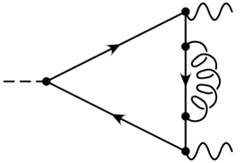
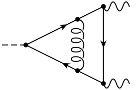
Figure 2: One- and some two-loop diagrams contribution to $H\to\gamma\gamma$. The dashed lines correspond to the Higgs boson, the wavy lines to the photons, the curly ones to the gluons and the straight ones to the quarks.

The physical amplitude is calculated via a projection on the physical states

$${\cal M}^{(\leq 2)}_{H\rightarrow\gamma\gamma}=\left.G^{(\leq 2)}_{HA_{\mu}A_{\nu}}(q_{1},q_{2})\epsilon^{\mu}(q_{1})\epsilon^{\nu}(q_{2})\right|_{q_{1}^{2}=q_{2}^{2}=0,(q_{1}+q_{2})^{2}=M^{2}_{H}}\,,$$ (2.12)

where $M_{H}$ is the Higgs boson mass and $\epsilon^{\mu}(q)$ denotes the polarization vector of the photon with momentum $q$.

The mass shell projection of the two-loop amplitude can be correctly performed only if the self-energy of the photon, ${\rm I}\!\Gamma^{(1)}_{A_{\sigma}A_{\rho}}(q)$, satisfies the well-known transversality condition $q^{\nu}{\rm I}\!\Gamma^{(1)}_{A_{\mu}A_{\nu}}(q)=0$. However, in a non-symmetric regularization scheme this property is in general not valid any longer. It has to be reestablished as will be explained in Section 3.

In order to obtain the complete set of one-loop counterterms, we observe that the regularized two-loop Green function $\Gamma^{(2)}_{HA_{\mu}A_{\nu}}(q_{1},q_{2})$ contains three different sub-divergences which require proper subtraction. Furthermore, since in general the regularization procedure breaks the symmetry, we are forced to introduce the following general counterterm Lagrangian

$${\cal L}^{CT}_{H\rightarrow\gamma\gamma} = \sum_{i}Z_{1}\,e\,Q_{i}A_{\mu}\bar{q}_{i}\gamma^{\mu}q_{i}+Z_{2}\bar{q}_{i}\not\!\partial q_{i}+Z_{m_{i}}Z_{2}m_{i}\bar{q}_{i}q_{i}+Z_{Y_{i}}Z_{2}Y_{i}H\bar{q}_{i}q_{i}\,,$$ (2.13)

where $H,A_{\mu},\bar{q}_{i}$ and $q_{i}$ are the Higgs boson, the photon and the fermion fields, respectively. The parameters $e,m_{i}$ and $Y_{i}$ are the gauge coupling, the masses and the Yukawa couplings of the fermions. In a symmetric regularization scheme the free parameters $Z_{1},Z_{2},Z_{m_{i}}$ and $Z_{Y_{i}}$ are related by means of QED-WTI. In a non-invariant regularization scheme this is not true any longer and these coefficients have to be fixed separately. For example, in Analytic Regularization [23], which we will use for the practical computation, the renormalization constants are Laurent-expanded in powers of the regulators. In our case it turns out that it is enough to introduce only one, $\lambda$ [24]. Then the renormalization constants read $Z_{\alpha}=\sum_{n\geq 0}Z^{(n)}_{\alpha}/\lambda^{n}$ ($\alpha=1,2,m_{i},Y_{i}$). The pole parts are removed by means of the minimal subtraction scheme and the finite parts, $Z^{(0)}_{\alpha}$, are fixed by the STIs.

In order to fix the one-loop counterterms explicitly, we have to consider the Green functions ${\rm I}\!\Gamma^{(1),QCD}_{A_{\mu}\bar{q}_{i}q_{i}}(\bar{p},p),{\rm I}\!\Gamma^{(1),QCD}_{H\bar{q}_{i}q_{i}}(\bar{p},p)$ and ${\rm I}\!\Gamma^{(1),QCD}_{\bar{q}_{i}q_{i}}(p)$ which arise as sub-diagrams of the two-loop graphs. The fermion self-energy ${\rm I}\!\Gamma^{(1),QCD}_{\bar{q}_{i}q_{i}}(p)$ contains the two independent parameters $Z_{2}$ and $Z_{m_{i}}$ which are not constrained by any STI. They can be fixed as usual either minimally, i.e. $Z^{(0)}_{2}=Z^{(0)}_{m_{i}}=0$, or by imposing on-shell renormalization conditions

$${\rm I}\!\Gamma^{(1),QCD}_{\bar{q}_{i}q_{i}}(\not\!p=m_{i})=0,~{}~{}~{}\left.\frac{\partial}{\partial\!\!\!\not p}{\rm I}\!\Gamma^{(1),QCD}_{\bar{q}_{i}q_{i}}(p)\right|_{\not\,p=m_{i}}=1.$$ (2.14)

The parameter $Z_{Y_{i}}$ is related to the mass renormalization constant, $Z_{m_{i}}$. In our specific example, where fermion mixing is absent, both parameters can be identified. $Z_{1}$ has to be fixed in terms of the STI which relates the vertex ${\rm I}\!\Gamma^{(1),QCD}_{A_{\mu}\bar{q}_{i}q_{i}}(\bar{p},p)$ to the fermion self-energy. By differentiating the identity w.r.t. the photon ghost field $c_{A}$ and the fermion fields $\bar{q}_{i}$ and $q_{i}$, one immediately gets

$$\frac{\delta^{3}{\cal S}({\rm I}\!\Gamma)^{(1),QCD}}{\delta c_{A}(-p-\bar{p})\delta\bar{q}_{i}(\bar{p})\delta{q}_{i}({p})}\Bigg{|}_{\phi=0}=$$ (2.15)

$$\mbox{}i(\bar{p}+p)^{\mu}{\rm I}\!\Gamma^{(1),QCD}_{A_{\mu}\bar{q}_{i}q_{i}}(\bar{p},p)+ieQ_{i}\left({\rm I}\!\Gamma^{(1),QCD}_{\bar{q}_{i}q_{i}}({p})-{\rm I}\!\Gamma^{(1),QCD}_{\bar{q}_{i}q_{i}}(-\bar{p})\right)$$

$$= 0\,,$$

which is equivalent to the simple WTI in QED. Note that this equation is only true as exclusively QCD corrections are considered at two-loop order.

After the one-loop counterterms are fixed, let us now focus on the Green function ${\rm I}\!\Gamma^{(i)}_{HA_{\mu}A_{\nu}}(q_{1},q_{2})$ ($i=1,2$) which is our prime interest. We again have to make sure that the finite parts of the counterterms are correctly fixed according to the STI. In fact, since the process $H\to\gamma\gamma$ has no tree-level contribution there is no free overall parameter which fixes the finite parts by using renormalization conditions.

According to rule 3 of the previous subsection, we consider the derivative of ${\cal S}({\rm I}\!\Gamma)=0$ w.r.t. the photon ghost field $c_{A}$, one photon $A_{\nu}$ and the Higgs boson $H$. As a result we obtain the identity which involves among others also the Green functions ${\rm I}\!\Gamma_{HA_{\mu}A_{\nu}}(q_{1},q_{2})$:

$$\frac{\delta^{3}{\cal S}({\rm I}\!\Gamma)}{\delta c_{A}(q_{1})\delta A_{\nu}(q_{2})\delta H(p)}\bigg{|}_{\phi=0}=$$ (2.16)

$$\mbox{}\left(-ic^{2}_{W}q_{1}^{\rho}-s_{W}{\rm I}\!\Gamma_{c_{A}W^{*,3}_{\rho}}(-q_{1})\right){\rm I}\!\Gamma_{A_{\rho}A_{\nu}H}(q_{2},p)$$

$$\mbox{}+\left(-ic_{W}s_{W}q_{1}^{\rho}+c_{W}{\rm I}\!\Gamma_{c_{A}W^{*,3}_{\rho}}(-q_{1})\right){\rm I}\!\Gamma_{Z_{\rho}A_{\nu}H}(q_{2},p)$$

$$\mbox{}+{\rm I}\!\Gamma_{c_{A}W^{*,3}_{\rho}H}(q_{2},p)\left(c_{W}{\rm I}\!\Gamma_{Z_{\rho}A_{\nu}}(q_{2})-s_{W}{\rm I}\!\Gamma_{A_{\rho}A_{\nu}}(q_{2})\right)$$

$$\mbox{}+{\rm I}\!\Gamma_{c_{A}W^{*,3}_{\rho}A_{\nu}}(p,q_{2})\left(c_{W}{\rm I}\!\Gamma_{Z_{\rho}H}(p)-s_{W}{\rm I}\!\Gamma_{A_{\rho}H}(p)\right)$$

$$\mbox{}+{\rm I}\!\Gamma_{c_{A}G^{*,0}}(-q_{1}){\rm I}\!\Gamma_{G^{0}A_{\nu}H}(q_{2},p)+{\rm I}\!\Gamma_{c_{A}HG^{*,0}}(p,q_{2}){\rm I}\!\Gamma_{G^{0}A_{\nu}}(q_{2})$$

$$\mbox{}+{\rm I}\!\Gamma_{c_{A}G^{*,0}A_{\nu}}(p,q_{2}){\rm I}\!\Gamma_{G^{0}H}(p)+{\rm I}\!\Gamma_{c_{A}H^{*}}(-q_{1}){\rm I}\!\Gamma_{HA_{\nu}H}(q_{2},p)$$

$$\mbox{}+{\rm I}\!\Gamma_{c_{A}HH^{*}}(p,q_{2}){\rm I}\!\Gamma_{HA_{\nu}}(q_{2})+{\rm I}\!\Gamma_{c_{A}H^{*}A_{\nu}}(p,q_{2}){\rm I}\!\Gamma_{HH}(p)$$

$$= 0\,.$$

Actually this equation constitutes a special case of the identity (B.4) derived in a more general context.

In the following we demonstrate how this equation simplifies for the special kind of corrections we are interested in. In order to disentangle consistently the QCD corrections from the Green functions appearing in the STI at a given order one can take the derivative of the latter w.r.t. the parameters of the $SU(3)$ colour group, namely $C_{A}$ and $C_{F}$. Furthermore, we can disentangle the contributions of the fermion loop from the contribution of the bosonic corrections as the coupling of ghost fields (as well as the external BRST sources $W^{*,3}_{\rho}$, $G^{*,0}$ and $H^{*}$) to the fermion lines occurs for the first time through two-loop electroweak interactions. Note that the Green functions ${\rm I}\!\Gamma_{Z_{\rho}H}$, ${\rm I}\!\Gamma_{HA_{\nu}}$, ${\rm I}\!\Gamma_{G^{0}A_{\nu}H}$ and ${\rm I}\!\Gamma_{G^{0}H}$ vanish at tree-, one- and two-loop level as they violate CP invariance. It is well-known that the CP symmetry is violated in the SM only through the Cabibbo-Kobayashi-Maskawa (CKM) matrix. Thus CP violation manifests itself in the scalar sector starting at the three-loop order. The last term in (2.16) vanishes if one restricts the analysis to fermionic contributions and their QCD corrections. Taking these simplifications into account we finally get for the first term of the r.h.s. of Eq. (2.16) expanded up to two loops

$$\left({\rm I}\!\Gamma_{c_{A}W^{*,3}_{\rho}}{\rm I}\!\Gamma_{A_{\rho}A_{\nu}H}\right)^{(\leq 2),ferm} = {\rm I}\!\Gamma^{(0)}_{c_{A}W^{*,3}_{\rho}}(-q_{1}){\rm I}\!\Gamma^{(1),ferm}_{A_{\rho}A_{\nu}H}(q_{2},p)+{\rm I}\!\Gamma^{(1)}_{c_{A}W^{*,3}_{\rho}}(-q_{1}){\rm I}\!\Gamma^{(1),ferm}_{A_{\rho}A_{\nu}H}(q_{2},p)$$ (2.17)

$$\mbox{}+{\rm I}\!\Gamma^{(0)}_{c_{A}W^{*,3}_{\rho}}(-q_{1}){\rm I}\!\Gamma^{(2),QCD}_{A_{\rho}A_{\nu}H}(q_{2},p)\,.$$

Note that the three-point function ${\rm I}\!\Gamma^{(0)}_{A_{\rho}A_{\nu}H}(q_{2},p)$ is absent at tree level. Further simplifications occur through the observation that the second term on the r.h.s. of Eq. (2.17) does not give any contribution since there is no room for QCD corrections. Please note that the one-loop Green function ${\rm I}\!\Gamma^{(1)}_{c_{A}W^{*,3}_{\rho}}$ does not contain any fermionic loop. In the same line of reasoning all terms except the ones in the first two lines of Eq. (2.16) drop out.

From the Lagrangian one obtains ${\rm I}\!\Gamma^{(0)}_{c_{A}W^{*,3}_{\rho}}(-q_{1})=is_{W}q_{1}^{\mu}$. This in combination with the accordingly simplified remaining terms of Eq. (2.16) finally lead us to the following STI

$$-iq_{1}^{\rho}{\rm I}\!\Gamma^{(i),ferm}_{A_{\rho}A_{\nu}H}(q_{2},p)=0\,,~{}~{}~{}~{}i=1,2\,.$$ (2.18)

This identity must be fulfilled at one- and two-loop order for the specific corrections we are interested in.

In Section 4 the breaking terms for these identities will be provided. Furthermore we will compute the amplitude in the analytical regularization scheme and we will show how the algebraic renormalization works for this two-loop example.

2.3 Background gauge fixing

As is well known the BFM [11] allows to derive the S-matrix elements in terms of Green functions with external background fields with the exception of fermion fields. The main simplification in the BFM results from the fact that the theory with background fields possesses two different invariances: the BRST symmetry, which involves quantum fields and ghosts, and the background gauge invariance. The latter provides several simplifications in the computation of physical amplitudes and in the renormalization procedure due to its linearity. The first systematic application of BFM in the SM for invariant regularizations at the one-loop level was presented in [25]. Our considerations regarding BFM, however, also apply in the case of noninvariant regularizations and also beyond the one-loop level. We focus on the practical aspects of the BFM which are relevant for higher-loop calculations. Further details on the theoretical advantages of the BFM can be found in [25, 26, 21].

The main difference between the STIs (2.6) and the WTIs for the background gauge invariance is due to the linearity of the latter. Linearity means that the WTIs are linear in the functional ${\rm I}\!\Gamma$ and therefore they relate Green functions of the same orders while for the STIs there is an interplay between higher and lower order radiative corrections.

To renormalize properly the SM in the background gauge, one needs to implement the equations of motion for the background fields at the quantum level. The most efficient way to this end is to extend the BRST symmetry to the background fields

$$s\hat{W}^{3}_{\mu}=\Omega^{3}_{\mu},~{}~{}~{}~{}s\Omega^{3}_{\mu}=0,~{}~{}~{}~{}s\hat{G}^{0}=\Omega^{0},~{}~{}~{}~{}s\Omega^{0}=0,$$

$$s\hat{W}^{\pm}_{\mu}=\Omega^{\pm}_{\mu},~{}~{}~{}~{}s\Omega^{\pm}_{\mu}=0,~{}~{}~{}s\hat{G}^{\pm}=\Omega^{\pm},~{}~{}~{}s\Omega^{\pm}=0,$$ (2.19)

$$s\hat{G}_{\mu}^{a}=\Omega^{a}_{\mu},~{}~{}~{}~{}~{}s\Omega^{a}_{\mu}=0,~{}~{}~{}~{}s\hat{H}=\Omega^{H},~{}~{}~{}~{}~{}s\Omega^{H}=0,$$

where $\Omega^{\pm}_{\mu},\Omega^{3}_{\mu}$ and $\Omega^{a}_{\mu}$ are (classical) vector fields with the same quantum numbers as the gauge bosons $W,Z$ and $G^{a}_{\mu}$, but ghost charge $-1$ (like an anti-ghost field). $\Omega^{\pm},\Omega^{0}$ and $\Omega^{H}$ are scalar fields with ghost number $-1$; in the following we will denote by $\Omega$ the complete set of these fields.

In the following we will denote with ${\rm I}\!\Gamma^{\prime}$ the effective action which depend on the $\Omega$ (and correspondently the ${\cal S}^{\prime}_{{\rm I}\!\Gamma}$ its Slavnov-Taylor operator) and with ${\rm I}\!\Gamma=\left.{\rm I}\!\Gamma^{\prime}\right|_{\Omega=0}$, i.e. by setting $\Omega$ to zero.

Therefore one has to modify correspondingly the STI

$${\cal S}^{\prime}({\rm I}\!\Gamma^{\prime})[\phi] = {\cal S}({\rm I}\!\Gamma^{\prime})[\phi]+\int\,\,{\rm d}^{4}x\Bigg{\{}\Omega^{3}_{\mu}\left[c_{W}\left(\frac{\delta{\rm I}\!\Gamma^{\prime}}{\delta\hat{Z}_{\mu}}-\frac{\delta{\rm I}\!\Gamma^{\prime}}{\delta Z_{\mu}}\right)-s_{W}\left(\frac{\delta{\rm I}\!\Gamma^{\prime}}{\delta\hat{A}_{\mu}}-\frac{\delta{\rm I}\!\Gamma^{\prime}}{\delta A_{\mu}}\right)\right]$$ (2.20)

$$\mbox{}+\Omega^{\pm}_{\mu}\left(\frac{\delta{\rm I}\!\Gamma^{\prime}}{\delta\hat{W}^{\mp}_{\mu}}-\frac{\delta{\rm I}\!\Gamma^{\prime}}{\delta W^{\mp}_{\mu}}\right)+\Omega^{a}_{\mu}\left(\frac{\delta{\rm I}\!\Gamma^{\prime}}{\delta\hat{G}^{a}_{\mu}}-\frac{\delta{\rm I}\!\Gamma^{\prime}}{\delta G^{a}_{\mu}}\right)$$

$$\mbox{}+\Omega^{\pm}\left(\frac{\delta{\rm I}\!\Gamma^{\prime}}{\delta\hat{G}^{\mp}}-\frac{\delta{\rm I}\!\Gamma^{\prime}}{\delta G^{\mp}}\right)+\Omega^{0}\left(\frac{\delta{\rm I}\!\Gamma^{\prime}}{\delta\hat{G}^{0}}-\frac{\delta{\rm I}\!\Gamma^{\prime}}{\delta{G}^{0}}\right)+\Omega^{H}\left(\frac{\delta{\rm I}\!\Gamma^{\prime}}{\delta\hat{H}}-\frac{\delta{\rm I}\!\Gamma^{\prime}}{\delta H}\right)\Bigg{\}}$$

$$= 0\,.$$

Here ${\cal S}({\rm I}\!\Gamma^{\prime})[\phi]$ are the STIs given in Eq. (2.6). Notice that also the scalar fields $G^{\pm}$, $G^{0}$ and $H$ are paired with their own background fields, $\hat{G}^{\pm},\hat{G}^{0}$ and $\hat{H}$ in order to extend the ‘t Hooft gauge fixing to a background gauge invariant one described in Appendix A.

To study how the effective action ${\rm I}\!\Gamma^{\prime}$ depends on $\hat{W}^{\pm}_{\mu}$, for instance, one has to derive the STI (2.20) with respect to the fields $\Omega^{\pm}_{\mu}$. After setting $\Omega^{\pm}_{\mu}=0$ one obtains

$$\left(\frac{\delta{\rm I}\!\Gamma}{\delta\hat{W}^{\mp}_{\mu}}-\frac{\delta{\rm I}\!\Gamma}{\delta W^{\mp}_{\mu}}\right)={\cal S}_{{\rm I}\!\Gamma}\left(\frac{\delta{\rm I}\!\Gamma^{\prime}}{\delta{\Omega}^{\mp}_{\mu}}\right)_{\Omega=0}\,,$$ (2.21)

where ${\cal S}_{{\rm I}\!\Gamma}$ is the linearized (conventional) Slavnov-Taylor operator of Eq. (A.8). These equations describe the relations between the quantum and the background fields and they supplement the STI and the WTI:

$${\cal S}\left({\rm I}\!\Gamma\right)=0,~{}~{}~{}~{}{\cal W}_{(\lambda)}({\rm I}\!\Gamma)=0$$ (2.22)

where ${\cal W}_{(\lambda)}$ is the WTI operator of the background gauge invariance (cf. Eq. (2.24)).

The space of counterterms and of possible breaking terms to the STI is enlarged by those monomials which contain the background fields $\hat{\phi}$ and the fields $\Omega$ in addition to the conventional fields $\phi$ and anti-fields $\phi^{*}$. This requires a new analysis.

In the calculation of the necessary counterterms, there are two main approaches. They only differ by the ordering in which the three equations in (2.21) and (2.22) are used.

1. We first use the WTI for the background gauge invariance and a subset of the conventional STIs (2.6). The only missing parts are counterterms which relate the two-point functions of the background field to the two-point functions of the quantum fields and for the two-point functions $\Gamma_{\phi^{*}\Omega}$, where $\phi^{*}$ is a generic anti-field. To fix these last counterterms one has to use the extended STI (2.20).

   Thus, to fix for example the counterterms for the two-point function for the quantum field $W^{\pm}_{\mu}$, one has to derive the STI (2.20) with respect to $\Omega^{\pm}_{\mu},\hat{W}^{\mp}_{\nu}$ and with respect to $\Omega^{\pm}_{\mu},W^{\mp}_{\nu}$:

   $${\rm I}\!\Gamma_{\hat{W}^{+}{W}^{-}}(p) = {\rm I}\!\Gamma_{W^{+}W^{-}}(p)+{\rm I}\!\Gamma_{\Omega^{+}W^{*,-}}(p){\rm I}\!\Gamma_{W^{+}W^{-}}(p)\,,$$

   $${\rm I}\!\Gamma_{\hat{W}^{+}\hat{W}^{-}}(p) = {\rm I}\!\Gamma_{W^{+}\hat{W}^{-}}(p)+{\rm I}\!\Gamma_{\Omega^{+}W^{*,-}}(p){\rm I}\!\Gamma_{W^{+}\hat{W}^{-}}(p)\,.$$ (2.23)

   These equations fix completely the two-point functions ${\rm I}\!\Gamma_{\hat{W}^{+}{W}^{-}}(p),{\rm I}\!\Gamma_{\hat{W}^{+}\hat{W}^{-}}(p)$ in terms of the quantum one ${\rm I}\!\Gamma_{W^{+}W^{-}}(p)$. Finally, in order to fix the counterterms for the two-point functions $\Gamma_{\phi^{*}\Omega}$ (a complete discussion has been given in [21]), one has to consider the derivative of (2.21) with respect to the anti-field $\phi^{*}$ and one ghost $c$. This conclude the algebraic renormalization program in the case of the BFM.

2. The second alternative approach exploits completely the use of the extended STI, namely equations of the type (2.21): Thus, one first computes all possible counterterms to restore the WTI, then one fixes the remaining counterterms by considering the functional derivative of the extended STI (2.20) with respect to $\Omega$, the background fields $\hat{\phi}$ and the quantum fields $\phi$. However, as in the former approach this cannot exhaust completely the algebraic renormalization program: One shows that one still needs a reduced set of STIs in addition which can be derived from the conventional STI (2.6). In particular, besides the Eqs. (2.21), one needs the STI to fix the anti-field part of the action. This guarantees that the BRST transformation are preserved to all orders.

In a practical analysis of a physical process where one has not to compute the same Green functions with the quantum fields replaced by the corresponding background fields nor vice versa, the first approach is favourable — as in the two phenomenological examples discussed in this paper. One can disregard all equations of the type (2.21). This simplifies the analysis significantly. A phenomenological example using the second approach will be discussed in a forthcoming publication. In Section 3.2 we discuss the analysis of the breaking terms in both methods within the BFM.

In order to single out the relevant WTI, we have to take into account the rules stated in Section 2.1. However, in the case of the background fields, the role of the ghost particles is played by the parameter of the infinitesimal background gauge transformations (see Appendix A). To each generator of the gauge group $SU_{C}(3)\times SU_{I}(2)\times U_{Y}(1)$ we consider the corresponding local infinitesimal parameters. They are denoted by $\lambda_{A}(x),\lambda_{Z}(x)$ and $\lambda_{\pm}(x)$ for the electroweak part and $\lambda_{a}(x)$ for the QCD sector. Thus, the functional WTI for the effective action ${\rm I}\!\Gamma^{\prime}$ reads:

$${\cal W}^{\prime}_{(\lambda)}({\rm I}\!\Gamma^{\prime}) = \sum_{\phi}\int{\rm d}^{4}x\left(\delta_{\lambda(x)}\phi\right)\frac{\delta{\rm I}\!\Gamma^{\prime}}{\delta\phi(x)}=\sum_{\alpha=A,Z\pm,a}\int{\rm d}^{4}x\lambda_{\alpha}(x){\cal W}^{\prime}_{\alpha}(x)({\rm I}\!\Gamma^{\prime})\,\,=\,\,0\,,$$ (2.24)

where the variations $\delta_{\lambda}\phi(x)$ are explicitly given in Appendix A (see Eqs. (• ‣ A)–(• ‣ A)). The sum runs over all possible fields and anti-fields. ${\cal W}^{\prime}_{\alpha}(\lambda)({\cal W}^{\prime}_{\alpha}(x))$ is called Ward-Takahashi operator and acts on the functional ${\rm I}\!\Gamma^{\prime}[\phi]$. An explicit expression is given in [25].

Concerning the rules of Section 2.1, only two slight modifications of the rules 3 and 4 are necessary:

• One has to differentiate the general WTI (2.24) w.r.t. the infinitesimal parameters $\lambda_{V}$ in order to get constraints on the Green functions involving the corresponding background gauge fields $\hat{V}$.

• To derive constraints on Green functions involving one ghost and one anti-field plus other quantum fields one either can derive a corresponding STI with rule 4 (i.e. differentiate Eq. (2.6) w.r.t. two ghost fields) or one can derive a linear WTI by differentiating w.r.t. one ghost field and one infinitesimal parameter $\lambda_{\alpha}$. We prefer to use the second version since linear WTIs are simpler to handle within our specific subtraction method (cf. Section 3.3). Note that this choice implies some assumptions on the wave function renormalization for multiplets of fields as will be explained in more detail in the example on $b\rightarrow s\gamma$ (cf. Section 5).

In connection to these modifications a remark is in order. If we consider a Green function with one gauge field, one ghost field and one anti-field (e.g., ${\rm I}\!\Gamma_{c_{A}W^{*,+}_{\mu}W^{-}_{\nu}}$) we have to differentiate the WTI (2.24) w.r.t. the ghost field, the anti-field and the infinitesimal parameter (which in the example is $\lambda_{-}$) associated to the gauge field. This provides an identity which fixes the considered Green function. In the case that no gauge field is involved (e.g., ${\rm I}\!\Gamma_{c_{A}\bar{q}^{*}q^{\prime}}$) one has to consider the background variation of the ghost field, of the anti-fields and of the quantum field (which in the example is $q^{\prime}$). Thus the WTI has to be differentiated w.r.t. $\delta_{\lambda}c_{A},\bar{q}^{*}$ and $q^{\prime}$, and $c_{A},\delta_{\lambda}\bar{q}^{*}$ and $q^{\prime}$, and $c_{A},\bar{q}^{*}$ and $\delta_{\lambda}q^{\prime}$. Some of the resulting WTIs coincide. One has to select the independent ones, but this can be easily done by inspection of the WTIs themselves.

At this point let us consider the example discussed in Appendix B the amplitude involving two gauge fields $V^{\mu}_{i}$ and one scalar field $\Phi$ in the context of the BFM. Thus we are able to compare the two approaches and to underline the differences.

In the framework of the BFM the two gauge fields, $V^{\mu}_{1}$ and $V^{\nu}_{2}$, and the scalar field $\Phi$ are replaced by their counterparts $\hat{V}^{\mu}_{1}$, $\hat{V}^{\nu}_{2}$ and $\hat{\Phi}$, respectively. As in the conventional gauge fixing the amplitude is built up by irreducible Green functions which in this case read ${\rm I}\!\Gamma_{\hat{V}^{\mu}_{i}\hat{V}^{\nu}_{j}}$ $(i,j=1,2)$, ${\rm I}\!\Gamma_{\hat{\Phi}\hat{\Phi}}$ and ${\rm I}\!\Gamma_{\hat{V}^{\mu}_{1}\hat{V}^{\nu}_{2}\hat{\Phi}}$. In the following we will denote irreducible Green functions where only external background fields are involved as background Green functions.

Let us in a first step consider the two-point function ${\rm I}\!\Gamma_{\hat{V}^{i}_{\mu}\hat{V}^{j}_{\nu}}(p)$. We get the following identities using (2.24) in combination with Eqs. (• ‣ A)–(• ‣ A):

$$\left.\frac{\delta^{2}{\cal W}_{(\lambda)}({\rm I}\!\Gamma)}{\delta\lambda_{V}^{i}(-p)\delta\hat{V}^{j}_{\nu}(p)}\right|_{\phi=0} = ip^{\mu}{\rm I}\!\Gamma_{\hat{V}^{i}_{\mu}\hat{V}^{j}_{\nu}}(p)+\sum_{\Phi^{\prime}}M_{i,\Phi^{\prime}}{\rm I}\!\Gamma_{\hat{\Phi}^{\prime}\hat{V}^{j}_{\nu}}(p)\,\,=\,\,0\,.$$ (2.25)

The sum runs over all Goldstone fields $G^{0}$ and $G^{\pm}$ with masses $M_{\pm,G^{\pm}}=\pm iM_{W}$, $M_{Z,G^{0}}=-M_{Z}$ and zero for all the other combinations. In the following the summation sign will be omitted. A comparison with the corresponding identity in the conventional formalism, Eq. (B.1), shows that Eq. (2.25) is linear in the Green functions. However, it requires the renormalization of the mixed two-point functions ${\rm I}\!\Gamma_{\hat{\Phi}^{\prime}\hat{V}^{j}_{\nu}}(p)$ which can be studied with the help of rule $3^{\prime}$:

$$\left.\frac{\delta^{2}{\cal W}_{(\lambda)}({\rm I}\!\Gamma)}{\delta\lambda_{V}^{i}(-p)\delta\hat{\Phi}(p)}\right|_{\phi=0} = ip^{\mu}{\rm I}\!\Gamma_{\hat{V}^{i}_{\mu}\hat{\Phi}}(p)+M_{i,\Phi^{\prime}}{\rm I}\!\Gamma_{\hat{\Phi}^{\prime}\hat{\Phi}}(p)\,\,=\,\,0\,.$$ (2.26)

Let us now come to the three-point function ${\rm I}\!\Gamma_{\hat{V}^{\mu}_{1}\hat{V}^{\nu}_{2}\hat{\Phi}}(p_{1},p_{2})$. From Eq. (2.24) we get

$$\left.\frac{\delta^{3}{\cal W}_{(\lambda)}({\rm I}\!\Gamma)}{\delta\lambda_{V}^{i}(-p_{1}-p_{2})\delta\hat{V}^{j}_{\nu}(p_{1})\delta\hat{\Phi}(p_{2})}\right|_{\phi=0}=$$ (2.27)

$$\mbox{}i\left(p_{1}+p_{2}\right)^{\mu}{\rm I}\!\Gamma_{\hat{V}^{i}_{\mu}\hat{V}^{j}_{\nu}\hat{\Phi}}(p_{1},p_{2})+M_{i,\Phi^{\prime}}{\rm I}\!\Gamma_{\hat{\Phi}^{\prime}\hat{V}^{j}_{\nu}\hat{\Phi}}(p_{1},p_{2})+f_{ijk}{\rm I}\!\Gamma_{\hat{V}^{k}_{\nu}\hat{\Phi}}(p_{2})+t_{i,\Phi\Phi^{\prime}}{\rm I}\!\Gamma_{\hat{\Phi^{\prime}}\hat{V}^{j}_{\nu}}(p_{1})$$

$$= 0\,,$$

where $f_{ijk}$ and $t_{i,\Phi\Phi^{\prime}}$ represent the structure constants, respectively, the generators of the gauge group in the representation for scalar fields. We refrain from listing them explicitly. In the above identity the two-point functions are already known and only the function ${\rm I}\!\Gamma_{\hat{\Phi}^{\prime}\hat{V}^{j}_{\nu}\hat{\Phi}}(p_{1},p_{2})$ is new. It is fixed by the WTI

$$\left.\frac{\delta^{3}{\cal W}_{(\lambda)}({\rm I}\!\Gamma)}{\delta\lambda_{V}^{i}(-p_{1}-p_{2})\delta\hat{\Phi}(p_{1})\delta\hat{\Phi}^{\prime}(p_{2})}\right|_{\phi=0}=$$ (2.28)

$$\mbox{}i\left(p_{1}+p_{2}\right)^{\mu}{\rm I}\!\Gamma_{\hat{V}^{i}_{\mu}\hat{\Phi}^{\prime}\hat{\Phi}}(p_{1},p_{2})+M_{i,\Phi^{\prime\prime}}{\rm I}\!\Gamma_{\hat{\Phi}^{\prime\prime}\hat{\Phi}\hat{\Phi}^{\prime}}(p_{1},p_{2})+t_{i,\Phi^{\prime}\Phi^{\prime\prime}}{\rm I}\!\Gamma_{\hat{\Phi}^{\prime\prime}\hat{\Phi}}(p_{1})+t_{i,\Phi\Phi^{\prime\prime}}{\rm I}\!\Gamma_{\hat{\Phi}^{\prime}\hat{\Phi}^{\prime\prime}}(-p_{2})$$

$$= 0\,,$$

where again the sum over $\Phi^{\prime\prime}$ takes the values $G^{0}$ and $G^{\pm}$.

The four equations (2.25), (2.26), (2.27) and (2.28) already form the complete set of identities needed for the computation of the amplitude. In fact, all identities are linear in ${\rm I}\!\Gamma$ and therefore they keep the same form to all orders. This also implies that the coefficients $f_{ijk},t_{i,\Phi\Phi^{\prime}}$ and $M_{i,\Phi}$ are not renormalized. Their renormalization is fixed from the renormalization conditions. Furthermore no Green function involving ghosts or anti-fields occur. Let us mention that instead of the four identities derived above roughly ten mostly non-linear STIs have to be analyzed in the conventional gauge fixing. Thus, in this case the BFM is obviously superior as compared to the conventional gauge fixing.

At this point a practical remark is in order: the obvious advantage of the BFM due the linearity of the WTIs is only valid at the highest order of the computation. In lower orders, i.e. in sub-diagrams, also quantum field Green functions are involved which makes it necessary to use all three types of identities, namely (2.20), (2.24) and (2.21), in general. Thus, in specific examples, the BFM may introduce more complications in the sub-diagrams in comparison with a conventional gauge fixing such that the advantages of the BFM at the highest loop level could get partly compensated. However, in the example of the two-loop corrections to $b\rightarrow s\gamma$, to be discussed in the next section, we will show that the analysis of the sub-diagrams within the BFM is still favourable compared with the analysis within a conventional gauge.

Let us finish this section with two practical remarks about the gauge fixing and renormalization conditions within the BFM.

In order to evaluate the S-matrix elements in the BFM a gauge fixing has to be chosen for the background gauge fields. However, this choice is completely independent from the gauge fixing used for the internal gauge fields. This allows for a more convenient choice oriented on the physical process. For instance, the BFM Green functions with external unphysical scalar bosons ($G^{0}$ and $G^{\pm}$), with external ghost fields as well as longitudinal gauge bosons can be neglected in the decomposition of S-matrix elements in terms of 1PI parts. This can be achieved via the use of the unitary gauge fixing for the BFM propagators (see [25] for explicit examples). The procedure can be implemented both for the electroweak and the QCD sector of the SM.

Besides the symmetries of the BFM one has to impose some renormalization conditions in order to unambiguously fix the finite parts of Green functions. It appears very useful to implement them in terms of background Green functions [21]. The relation between the renormalization conditions for the background Green functions and those for the quantum fields are considered in [21].

2.4 Example 2: Green Functions, STIs and WTIs for the $b\rightarrow s\gamma$

In this section, we briefly describe the decomposition of the S-matrix elements for the process $b\rightarrow s\gamma$ in terms of 1PI functions at two-loop approximation. Simplifications concerning the renormalization procedure are discussed in the context of the BFM. We explicitly derive all WTIs and STIs constraining the counterterms at the one- and two-loop level for this specific process .

The decomposition of the (truncated) connected BFM Green functions in terms of 1PI functions can be split into two contributions. The first one, $G^{(2),vertex}_{\hat{A}_{\mu}b\bar{s}}(p_{b},p_{s})$, contains the flavour changing neutral current (FCNC) vertex corrections whereas the second one, $G^{(2),s.e.}_{\hat{A}_{\mu}b\bar{s}}(p_{b},p_{s})$, the FCNC self-energies:

$$G^{(2)}_{\hat{A}_{\mu}b\bar{s}}(p_{b},p_{s}) = G^{(2),vertex}_{\hat{A}_{\mu}b\bar{s}}(p_{b},p_{s})+G^{(2),s.e.}_{\hat{A}_{\mu}b\bar{s}}(p_{b},p_{s})\,.$$ (2.29)

Remember that for the background fields we have chosen to use the unitary gauge in order to avoid external unphysical particles. Then the two contributions are given by:

$$G^{(2),vertex}_{\hat{A}_{\mu}b\bar{s}}(p_{b},p_{s}) = {\rm I}\!\Gamma^{(2)}_{\hat{A}_{\mu}b\bar{s}}+{\rm I}\!\Gamma^{(1)}_{\hat{A}_{\mu}\hat{A}_{\sigma}}G^{(0)}_{\hat{A}_{\sigma}\hat{A}_{\nu}}{\rm I}\!\Gamma^{(1)}_{\hat{A}_{\nu}b\bar{s}}+{\rm I}\!\Gamma^{(1)}_{b\bar{b}}G^{(0)}_{b\bar{b}}{\rm I}\!\Gamma^{(1)}_{\hat{A}_{\mu}b\bar{s}}+{\rm I}\!\Gamma^{(1)}_{\hat{A}_{\mu}b\bar{s}}G^{(0)}_{s\bar{s}}{\rm I}\!\Gamma^{(1)}_{s\bar{s}}$$ (2.30)

$$\mbox{}+{\rm I}\!\Gamma^{(1)}_{\hat{A}_{\mu}\hat{H}}G^{(0)}_{\hat{H}\hat{H}}{\rm I}\!\Gamma^{(1)}_{\hat{H}b\bar{s}}+{\rm I}\!\Gamma^{(1)}_{\hat{A}_{\mu}\hat{Z}_{\sigma}}G^{(0)}_{\hat{Z}_{\sigma}\hat{Z}_{\nu}}{\rm I}\!\Gamma^{(1)}_{\hat{Z}_{\nu}b\bar{s}}\,,$$

$$G^{(2),s.e.}_{\hat{A}_{\mu}b\bar{s}}(p_{b},p_{s}) = {\rm I}\!\Gamma^{(0)}_{\hat{A}_{\mu}b\bar{b}}G^{(0)}_{b\bar{b}}{\rm I}\!\Gamma^{(2)}_{b\bar{s}}+{\rm I}\!\Gamma^{(2)}_{b\bar{s}}G^{(0)}_{s\bar{s}}{\rm I}\!\Gamma^{(0)}_{\hat{A}_{\mu}s\bar{s}}+{\rm I}\!\Gamma^{(1)}_{\hat{A}_{\mu}b\bar{b}}G^{(0)}_{b\bar{b}}{\rm I}\!\Gamma^{(1)}_{b\bar{s}}+{\rm I}\!\Gamma^{(1)}_{b\bar{s}}G^{(0)}_{s\bar{s}}{\rm I}\!\Gamma^{(1)}_{\hat{A}_{\mu}s\bar{s}}$$ (2.31)

$$\mbox{}+{\rm I}\!\Gamma^{(1)}_{\hat{A}_{\mu}\hat{H}}{\rm I}\!\Gamma^{(1)}_{b\bar{s}}G^{(0)}_{s\bar{s}}{\rm I}\!\Gamma^{(0)}_{\hat{H}s\bar{s}}+{\rm I}\!\Gamma^{(1)}_{\hat{A}_{\mu}\hat{H}}{\rm I}\!\Gamma^{(0)}_{\hat{H}b\bar{b}}G^{(0)}_{b\bar{b}}{\rm I}\!\Gamma^{(1)}_{b\bar{s}}$$

$$\mbox{}+{\rm I}\!\Gamma^{(1)}_{\hat{A}_{\mu}\hat{Z}_{\nu}}G^{(0)}_{b\bar{b}}{\rm I}\!\Gamma^{(1)}_{b\bar{s}}{\rm I}\!\Gamma^{(0)}_{\hat{Z}_{\nu}s\bar{s}}+{\rm I}\!\Gamma^{(1)}_{\hat{A}_{\mu}\hat{Z}_{\nu}}{\rm I}\!\Gamma^{(0)}_{\hat{Z}_{\nu}b\bar{b}}G^{(0)}_{b\bar{b}}{\rm I}\!\Gamma^{(1)}_{b\bar{s}}\,.$$

We recall that $G^{(0)}_{ij}$ denotes the tree-level propagators and ${\rm I}\!\Gamma$ the irreducible Green functions. After projection on the physical states, the contributions from the $\gamma-Z$ and $\gamma-H$ mixings vanish because of the WTI

$$\left.\frac{\delta^{2}{\cal W}_{(\lambda)}({\rm I}\!\Gamma)}{\delta\lambda_{A}(-p)\delta\hat{H}(p)}\right|_{\phi=0} = ip_{\mu}{\rm I}\!\Gamma_{\hat{A}_{\mu}\hat{H}}(p)\,\,=\,\,0\,,$$ (2.32)

where an analogous equation holds for ${\rm I}\!\Gamma_{\hat{A}_{\mu}\hat{Z}_{\nu}}$. Thus the second line in Eq. (2.30) and the second and third lines of Eq. (2.31) drop out from the amplitudes.

Let us in a first step consider the two-loop contribution to the $b\rightarrow s\gamma$ amplitude and derive the corresponding WTI. According to our rules we have to replace the photon field, $A_{\mu}$, by the corresponding infinitesimal parameter of $U_{Q}(1)$, $\lambda_{A}$. Furthermore we have to take the derivative of Eq. (2.24) w.r.t. $\lambda_{A}$, $b$ and $s$. Using the formulae (• ‣ A)–(• ‣ A) we obtain

$$\left.\frac{\delta^{3}{\cal W}_{(\lambda)}({\rm I}\!\Gamma)^{(2)}}{\delta\lambda_{A}(-p_{s}-p_{b})\delta\bar{s}(p_{s})\delta b(p_{b})}\right|_{\phi=0}=$$ (2.33)

$$\mbox{}i(p_{s}+p_{b})^{\mu}{\rm I}\!\Gamma^{(2)}_{\hat{A}_{\mu}\bar{s}b}(p_{s},p_{b})+ieQ_{d}\left({\rm I}\!\Gamma^{(2)}_{\bar{s}b}(p_{b})-{\rm I}\!\Gamma^{(2)}_{\bar{s}b}(-p_{s})\right)$$

$$= 0\,,$$

where $Q_{d}$ is the charge of the down-type quarks and $p_{b}$ and $p_{s}$ are the in-going momenta of the quark lines. This identity (for a one-loop analysis see also [27, 28]) can be used to fix the overall counterterms defined through

$${\cal L}^{(2),CT}_{b\rightarrow s\gamma}=Z^{(2)}_{L,1}\hat{A}_{\lambda}\bar{s}\gamma^{\lambda}P_{L}b+Z^{(2)}_{L,2}\bar{s}\not\!\partial P_{L}b+Z^{(2)}_{R,1}\hat{A}_{\lambda}\bar{s}\gamma^{\lambda}P_{R}b+Z^{(2)}_{2}\bar{s}\not\!\partial P_{R}b+{\rm h.c.}\,,$$ (2.34)

where the $Z$ factors, in general, contain finite and divergent contributions. Clearly the same Lagrangian also holds at one-loop order. $P_{L/R}=(1\mp\gamma_{5})/2$ are the projectors on the left- and right-handed components. Note that for an invariant regularization scheme no counterterm at all is needed for the Green function ${\rm I}\!\Gamma^{(2)}_{\hat{A}_{\mu}b\bar{s}}(p_{b},p_{s})$. However, if the regularization scheme breaks the identity (2.33), it can be restored with the help of non-invariant counterterms in (2.34).

Figure 3: One-loop diagrams contributing to $b\to s\gamma$. In order to obtain the two-loop diagrams one-loop corrections to each vertex and internal propagator have to be considered. The two external fermion lines represent the $b$, respectively, the $s$ quark and the external wiggled line the background photon, $\hat{A}_{\mu}$.

Let us now have a closer look to the sub-divergences. From the topological structure of the two-loop diagrams with only external background gauge fields, which are contained in ${\rm I}\!\Gamma^{(2)}_{\hat{A}_{\mu}b\bar{s}}$ (cf. Fig. 3), it is evident that the 1PI three- and four-point Green functions with external quantum, respectively, ghost fields do not appear at one-loop order:

$${\rm I}\!\Gamma^{(1)}_{V^{a}_{\mu}V^{b}_{\nu}V^{c}_{\rho}}\,,\qquad{\rm I}\!\Gamma^{(1)}_{V^{a}_{\mu}V^{b}_{\nu}V^{c}_{\rho}V^{d}_{\sigma}}\,,\qquad{\rm I}\!\Gamma^{(1)}_{V^{a}_{\mu}\bar{c}^{b}c^{c}}\,.$$ (2.35)

Here $V^{a}_{\mu}$ are the vector quantum fields and $c^{a}$ are ghost fields. Also the Green functions where the vector fields are replaced by scalar fields do not contribute. Actually the renormalization of sub-divergences with more then two quantum fields enter the calculation only at three-loop order. Thus, we only have to consider Green functions which are either sub-diagrams of ${\rm I}\!\Gamma^{(2)}_{\hat{A}_{\mu}b\bar{s}}$ or diagrams occurring in (2.30) and  (2.31) respectively. Concerning the three-point diagrams the following functions have to be taken into account:

$$\begin{array}[]{llll}{\rm I}\!\Gamma^{(1)}_{\hat{A}_{\mu}\bar{s}b}(p_{s},p_{b})\,,&{\rm I}\!\Gamma^{(1)}_{\hat{A}_{\mu}\bar{q}_{2}q_{1}}(p_{2},p_{1})\,,&{\rm I}\!\Gamma^{(1)}_{\hat{A}_{\mu}W^{+}_{\nu}W^{-}_{\rho}}(p_{+},p_{-})\,,&{\rm I}\!\Gamma^{(1)}_{\hat{A}_{\mu}G^{+}G^{-}}(p_{+},p_{-})\,,\\ \\ {\rm I}\!\Gamma^{(1)}_{\hat{A}_{\mu}G^{+}W^{-}_{\nu}}(p_{+},p_{-})\,,&{\rm I}\!\Gamma^{(1)}_{\hat{A}_{\mu}W^{+}_{\nu}G^{-}}(p_{+},p_{-})\,,&{\rm I}\!\Gamma^{(1)}_{W^{+}_{\mu}\bar{q}_{2}q_{1}}(p_{2},p_{1})\,,&{\rm I}\!\Gamma^{(1)}_{G^{+}\bar{q}_{2}q_{1}}(p_{2},p_{1})\,.\end{array}$$ (2.39)

The two-point functions

$$\begin{array}[]{lll}{\rm I}\!\Gamma^{(1)}_{\bar{s}b}(p_{s},p_{b})\,,&{\rm I}\!\Gamma^{(1)}_{\bar{q}_{2}q_{1}}(p_{2},p_{1})\,,&{\rm I}\!\Gamma^{(1)}_{W^{+}_{\nu}W^{-}_{\rho}}(p_{+},p_{-})\,,\\ \\ {\rm I}\!\Gamma^{(1)}_{G^{+}G^{-}}(p_{+},p_{-})\,,&{\rm I}\!\Gamma^{(1)}_{G^{+}W^{-}_{\mu}}(p_{+},p_{-})\,,&{\rm I}\!\Gamma^{(1)}_{W^{+}_{\mu}G^{-}}(p_{+},p_{-})\,,\end{array}$$ (2.43)

appear as self-energies in the two-loop graphs. In Eqs. (2.39) and  (2.43) $q_{1}$ and $q_{2}$ are two generic quark fields. Notice that the Green functions ${\rm I}\!\Gamma_{\hat{A}_{\mu}G^{+}W^{-}_{\nu}}$ and ${\rm I}\!\Gamma_{\hat{A}_{\mu}W^{+}_{\nu}G^{-}}$ are absent at tree level. This is a consequence of the choice for the gauge fixing and the background gauge invariance. At one-loop level, however, contributions may appear as soon as a non-invariant regularization scheme is used.

By inspection of Eqs. (2.39) and (2.43), we see that the same Green functions with the quantum fields replaced by the corresponding background fields never occur. This implies that the STI identities (2.21) relating background and quantum fields are irrelevant for the practical analysis of this specific process and we can restrict ourselves to the conventional STI and the WTI. In Section 3.2 we present a general discussion on this point.

Thus, let us discuss the STIs and WTIs which constrain the relevant sub-diagrams. Using our rules for the BFM we are able to derive the complete set of identities. For the three-point functions involving background photon field WTIs are used whereas only a reduced set of STIs for three-point functions and two-point functions are indeed necessary.

We start with the WTIs. From (2.24) one gets:

$$\left.\frac{\delta^{3}{\cal W}_{(\lambda)}({\rm I}\!\Gamma)^{(1)}}{\delta\lambda_{A}(-p_{1}-p_{2})\delta\bar{q}_{2}(p_{2})\delta q_{1}(p_{1})}\right|_{\phi=0}=$$ (2.44)

$$\mbox{}i\left(p_{2}+p_{{1}}\right)^{\mu}{\rm I}\!\Gamma^{(1)}_{\hat{A}_{\mu}\bar{q}_{2}q_{1}}(p_{2},p_{{1}})+ieQ_{q}\left({\rm I}\!\Gamma^{(1)}_{\bar{q}_{2}q_{1}}(p_{1})-{\rm I}\!\Gamma^{(1)}_{\bar{q}_{2}q_{1}}(-p_{2})\right)$$

$$= 0\,,$$

which is the analogue equation to (2.33). Here, however, $q_{1}$ and $q_{2}$ refer to any type of quark fields. As already mentioned above, an advantage of the BFM is the linearity of the identities w.r.t. ${\rm I}\!\Gamma$. This allows to disentangle easily the fermionic corrections from the bosonic ones. In fact, in the same way as for the $H\rightarrow\gamma\gamma$, we can select the independent contributions and introduce the corresponding counterterms. Notice furthermore that no ghosts are involved. In the case of conventional gauge fixing the identity (2.44) would be replaced by a STI obtained by differentiating w.r.t. $c_{A},q_{1}$ and $\bar{q}_{2}$. Already at one-loop order this identity would require the computation of Green functions involving ghost particles and off-shell quark fields.

The other Green functions of Eq. (2.39) involving background fields are constrained by the following WTI

$$\left.\frac{\delta^{3}{\cal W}_{(\lambda)}({\rm I}\!\Gamma)^{(1)}}{\delta\lambda_{A}(-p_{+}-p_{-})\delta W^{+}_{\rho}(p_{+})\delta W^{-}_{\sigma}(p_{-})}\right|_{\phi=0}=$$ (2.45)

$$\mbox{}i\left(p_{+}+p_{-}\right)^{\mu}{\rm I}\!\Gamma^{(1)}_{\hat{A}_{\mu}W^{+}_{\rho}W^{-}_{\sigma}}(p_{+},p_{-})-ie\left({\rm I}\!\Gamma^{(1)}_{W^{+}_{\rho}W^{-}_{\sigma}}(p_{-})-{\rm I}\!\Gamma^{(1)}_{W^{+}_{\rho}W^{-}_{\sigma}}(-p_{+})\right)$$

$$= 0\,,$$

$$\left.\frac{\delta^{3}{\cal W}_{(\lambda)}({\rm I}\!\Gamma)^{(1)}}{\delta\lambda_{A}(-p_{+}-p_{-})\delta G^{+}(p_{+})\delta G^{-}(p_{-})}\right|_{\phi=0}=$$ (2.46)

$$\mbox{}i\left(p_{+}+p_{-}\right)^{\mu}{\rm I}\!\Gamma^{(1)}_{\hat{A}_{\mu}G^{+}G^{-}}(p_{+},p_{-})-ie\left({\rm I}\!\Gamma^{(1)}_{G^{+}G^{-}}(p_{-})-{\rm I}\!\Gamma^{(1)}_{G^{+}G^{-}}(-p_{+})\right)$$

$$= 0\,,$$

$$\left.\frac{\delta^{3}{\cal W}_{(\lambda)}({\rm I}\!\Gamma)^{(1)}}{\delta\lambda_{A}(-p_{+}-p_{-})\delta W^{+}_{\rho}(p_{+})\delta G^{-}(p_{-})}\right|_{\phi=0}=$$ (2.47)

$$\mbox{}i\left(p_{+}+p_{-}\right)^{\mu}{\rm I}\!\Gamma^{(1)}_{\hat{A}_{\mu}W^{+}_{\rho}G^{-}}(p_{+},p_{-})-ie\left({\rm I}\!\Gamma^{(1)}_{W^{+}_{\rho}G^{-}}(p_{-})-{\rm I}\!\Gamma^{(1)}_{W^{+}_{\rho}G^{-}}(-p_{+})\right)$$

$$= 0\,,$$

and their hermitian counterparts.

According to our third rule of Section 2.1 for the Green functions ${\rm I}\!\Gamma_{\hat{A}_{\mu}W^{+}_{\nu}W^{-}_{\rho}}(p_{+},p_{-})$, ${\rm I}\!\Gamma_{\hat{A}_{\mu}W_{\nu}^{+}G^{-}}(p_{+},p_{-})$, ${\rm I}\!\Gamma_{\hat{A}_{\mu}G^{+}W_{\rho}^{-}}(p_{+},p_{-})$ and ${\rm I}\!\Gamma_{\hat{A}_{\nu}G^{+}G^{-}}(p_{+},p_{-})$ of the above equations one has to derive new STIs. For instance, one gets

$$\frac{\delta^{2}{\cal S}({\rm I}\!\Gamma)}{\delta\hat{A}_{\mu}(-p_{+}-p_{-})\delta c^{+}(p_{+})\delta W^{-}_{\rho}(p_{-})}\bigg{|}_{\phi=0}=$$ (2.48)

$$\mbox{}{\rm I}\!\Gamma_{\hat{A}_{\mu}c^{+}W^{*,-}_{\nu}}(p_{+},p_{-}){\rm I}\!\Gamma_{W^{+}_{\nu}W^{-}_{\rho}}(p_{-})+{\rm I}\!\Gamma_{\hat{A}_{\mu}c^{+}G^{*,-}}(p_{+},p_{-}){\rm I}\!\Gamma_{G^{+}W^{-}_{\rho}}(p_{-})$$

$$\mbox{}+{\rm I}\!\Gamma_{c^{+}W^{*,-}_{\nu}}(-p_{+}){\rm I}\!\Gamma_{\hat{A}_{\mu}W^{+}_{\nu}W^{-}_{\rho}}(p_{+},p_{-})+{\rm I}\!\Gamma_{c^{+}G^{*,-}}(-p_{+}){\rm I}\!\Gamma_{\hat{A}_{\mu}G^{+}W^{-}_{\rho}}(p_{+},p_{-})$$

$$= 0\,,$$

where the new Green functions ${\rm I}\!\Gamma_{\hat{A}_{\mu}c^{+}W^{*,-}_{\nu}}(p_{+},p_{-})$ and ${\rm I}\!\Gamma_{\hat{A}_{\mu}c^{+}G^{*,-}}(p_{+},p_{-})$ emerge. Clearly, also the STIs (2.48) can be spoiled by the radiative corrections and therefore it must be restored by suitable counterterms. However, it turns out that due to the consistency conditions (see Section 3.2) such STIs deliver no independent constraints. They are automatically preserved if the STIs for the two-point functions (discussed below (2.4)), the WTIs (2.45)–(2.47), and the WTIs involving the new Green functions ${\rm I}\!\Gamma_{\hat{A}_{\mu}c^{+}W^{*,-}_{\nu}}(p_{+},p_{-})$ and ${\rm I}\!\Gamma_{\hat{A}_{\mu}c^{+}G^{*,-}}(p_{+},p_{-})$ have been restored. These new WTIs are obtained by differentiating the WTI (2.24) w.r.t. $\lambda_{A}\,,c^{+}(p_{+})\,$ and $W^{*,-}_{\nu}(p_{-})$ and w.r.t. $\lambda_{A}\,,c^{+}(p_{+})$ and $G^{*,-}(p_{-})$:

$$\left.\frac{\delta^{3}{\cal W}_{(\lambda)}({\rm I}\!\Gamma)^{(1)}}{\delta\lambda_{A}(-p_{+}-p_{-})\delta c^{+}(p_{+})\delta W^{*,-}_{\nu}(p_{-})}\right|_{\phi=0}=$$ (2.49)

$$\mbox{}i\left(p_{+}+p_{-}\right)^{\mu}{\rm I}\!\Gamma^{(1)}_{\hat{A}_{\mu}c^{+}W^{*,-}_{\nu}}(p_{+},p_{-})-ie\left({\rm I}\!\Gamma^{(1)}_{c^{+}W^{*,-}_{\nu}}(p_{-})-{\rm I}\!\Gamma^{(1)}_{c^{+}W^{*,-}_{\nu}}(-p_{+})\right)$$

$$= 0\,,$$

$$\left.\frac{\delta^{3}{\cal W}_{(\lambda)}({\rm I}\!\Gamma)^{(1)}}{\delta\lambda_{A}(-p_{+}-p_{-})\delta c^{+}(p_{+})\delta G^{*,-}(p_{-})}\right|_{\phi=0}=$$ (2.50)

$$\mbox{}i\left(p_{+}+p_{-}\right)^{\mu}{\rm I}\!\Gamma^{(1)}_{\hat{A}_{\mu}c^{+}G^{*,-}}(p_{+},p_{-})-ie\left({\rm I}\!\Gamma^{(1)}_{c^{+}G^{*,-}}(p_{-})-{\rm I}\!\Gamma^{(1)}_{c^{+}G^{*,-}}(-p_{+})\right)$$

$$= 0\,.$$

These WTIs do not involve any new Green functions since the two-point functions ${\rm I}\!\Gamma^{(1)}_{c^{+}W^{*,-}_{\nu}}$ and ${\rm I}\!\Gamma^{(1)}_{c^{+}G^{*,-}}$ are already fixed by means of the Faddeev-Popov equations (B.2) as discussed in Appendix B. Notice that only the first equation of (2.49) can be broken by the radiative corrections since the second one involves (by Lorentz invariance) only finite quantities.

To restore the identities of the sub-diagrams, we need a complete set of counterterms. It is convenient to divide them into three different sets

$${\cal L}^{(1)}_{b\rightarrow s\gamma}={\cal L}^{(1),WTI}_{b\rightarrow s\gamma}+{\cal L}^{(1),STI}_{b\rightarrow s\gamma}+{\cal L}^{(1),INV}_{b\rightarrow s\gamma}\,,$$ (2.51)

organized in such a way that

$${\cal W}_{(\lambda)}\left(\int{\rm d}^{4}x{\cal L}^{(1),STI}_{b\rightarrow s\gamma}\right)\,\,=\,\,{\cal W}_{(\lambda)}\left(\int{\rm d}^{4}x{\cal L}^{(1),INV}_{b\rightarrow s\gamma}\right) = 0\,,$$

$${\cal S}_{0}\left(\int{\rm d}^{4}x{\cal L}^{(1),INV}_{b\rightarrow s\gamma}\right) = 0\,.$$ (2.52)

This triangular organization of the counterterms ensures that it is possible to restore the WTIs by only fixing the coefficients of ${\cal L}^{(1),WTI}_{b\rightarrow s\gamma}$. The counterterms ${\cal L}^{(1),STI}_{b\rightarrow s\gamma}$ and ${\cal L}^{(1),INV}_{b\rightarrow s\gamma}$ are invariant under the background gauge transformations. ${\cal L}^{(1),STI}_{b\rightarrow s\gamma}$ is necessary to restore the STIs and with the help of ${\cal L}^{(1),INV}_{b\rightarrow s\gamma}$ the renormalization conditions can be fulfilled. In Section 3.2 and in Appendix C we will prove with the help of the consistency conditions that this procedure is always possible provided no anomalies occur.

The complete list of counterterms for three-point functions needed to restore the WTIs is given by

$${\cal L}^{(1),WTI}_{b\rightarrow s\gamma} = Z^{(1)}_{3}\hat{A}_{\lambda}\hat{\nabla}^{\mu}W^{+,\lambda}W^{-}_{\mu}+Z^{(1)}_{4}\hat{A}_{\lambda}\hat{\nabla}^{\mu}W^{+}_{\mu}W^{-,\lambda}+Z^{(1)}_{5}\hat{A}_{\lambda}W^{+,\lambda}\hat{\nabla}^{\mu}W^{-}_{\mu}$$ (2.53)

$$\mbox{}+Z^{(1)}_{6}\left(\hat{A}_{\lambda}\hat{\nabla}^{\lambda}W^{+}_{\mu}W^{-,\mu}+\hat{A}_{\lambda}W^{+,\mu}\hat{\nabla}^{\lambda}W^{-}_{\mu}\right)+Z^{(1)}_{7}\hat{A}_{\lambda}W^{+}_{\mu}\hat{\nabla}^{\mu}W^{-}_{\lambda}$$

$$\mbox{}+Z^{(1)}_{8}\left(\epsilon_{\mu\nu\lambda\sigma}\hat{A}^{\lambda}W^{+,\mu}\hat{\nabla}^{\sigma}W^{-,\nu}-\epsilon_{\mu\nu\lambda\sigma}\hat{A}^{\lambda}W^{-,\mu}\hat{\nabla}^{\sigma}W^{+,\nu}\right)$$

$$\mbox{}+Z^{(1)}_{9}\hat{A}_{\lambda}G^{+}\hat{\nabla}^{\lambda}G^{-}+Z^{(1)}_{10}\hat{A}_{\lambda}G^{-}\hat{\nabla}^{\lambda}G^{+}+Z^{(1)}_{11}\hat{A}_{\lambda}G^{+}W^{-}_{\lambda}$$

$$\mbox{}+Z^{(1)}_{12}\hat{A}_{\lambda}G^{-}W^{+}_{\lambda}+\left(Z^{(1)}_{13}\hat{A}_{\lambda}\bar{s}P_{L}\gamma^{\lambda}b+Z^{(1)}_{14}\hat{A}_{\lambda}\bar{s}P_{R}\gamma^{\lambda}b+\right.$$

$$\mbox{}+\left.Z^{(1)}_{15}\hat{A}_{\lambda}\bar{q}_{2}P_{L}\gamma^{\lambda}q_{1}+Z^{(1)}_{16}\hat{A}_{\lambda}\bar{q}_{2}P_{R}\gamma^{\lambda}q_{1}+{\rm h.c.}\right)$$

$$\mbox{}+Z^{(1)}_{17}\hat{A}_{\lambda}c^{+}W^{*,-}_{\lambda}+Z^{(1)}_{18}\hat{A}_{\lambda}c^{-}W^{*,+}_{\lambda}\,,$$

where $\hat{\nabla}$ is the covariant derivative w.r.t. $U_{Q}(1)$. These counterterms correspond to the various Green functions occurring in the WTIs (2.44)–(2.47) and in the WTI (2.49). In Eq. (2.53) they are partially written in covariant form w.r.t. $U_{Q}(1)$ and also include counterterms to the WTIs which, however, are not relevant for our specific process under consideration. They would be needed, e.g., for the calculation of four-point functions like ${\rm I}\!\Gamma_{A_{\mu}A_{\nu}W^{+}_{\rho}W^{-}_{\sigma}}$. We note that this is the preferable basis for counterterms in order to analyze the renormalization of the whole model [21].

Besides the WTIs, we also have to take into account the following STIs. The general form for the two-point functions is also discussed in Appendix B. In Eqs. (B.1) and (B.2) they are given for a generic gauge field, $V_{\mu}$, and a generic scalar field $\Phi$. Note, that the Faddeev-Popov equation has to be used in order to obtain this simple form

$$\frac{\delta^{2}{\cal S}({\rm I}\!\Gamma)}{\delta c^{+}(-p)\delta W^{-}_{\mu}(p)}\bigg{|}_{\phi=0} = {\rm I}\!\Gamma_{c^{+}W^{*,-}_{\nu}}(p){\rm I}\!\Gamma_{W^{+}_{\nu}W^{-}_{\mu}}(p)+{\rm I}\!\Gamma_{c^{+}G^{*,-}}(p){\rm I}\!\Gamma_{G^{+}W^{-}_{\mu}}(p)\,\,=\,\,0\,,$$

$$\frac{\delta^{2}{\cal S}({\rm I}\!\Gamma)}{\delta c^{+}(-p)\delta G^{-}(p)}\bigg{|}_{\phi=0} = {\rm I}\!\Gamma_{c^{+}W^{*,-}_{\nu}}(p){\rm I}\!\Gamma_{W^{+}_{\nu}G^{-}}(p)+{\rm I}\!\Gamma_{c^{+}G^{*,-}}(p){\rm I}\!\Gamma_{G^{+}G^{-}}(p)\,\,=\,\,0\,,$$ (2.54)

which at one-loop order become

$${\rm I}\!\Gamma^{(1)}_{c^{+}W^{*,-}_{\nu}}(p)(i\,M_{W}^{2}\,g_{\nu\mu})+i\,p_{\nu}{\rm I}\!\Gamma^{(1)}_{W^{+}_{\nu}W^{-}_{\mu}}(p)+{\rm I}\!\Gamma^{(1)}_{c^{+}G^{*,-}}(p)(-i\,p_{\mu}\,M_{W})+i\,M_{W}\,{\rm I}\!\Gamma^{(1)}_{G^{+}W^{-}_{\mu}}(p) = 0\,,$$

$${\rm I}\!\Gamma^{(1)}_{c^{+}W^{*,-}_{\nu}}(p)(-i\,p_{\nu}M_{W})+i\,p_{\nu}\,{\rm I}\!\Gamma^{(1)}_{W^{+}_{\nu}G^{-}}(p)+{\rm I}\!\Gamma^{(1)}_{c^{+}G^{*,-}}(p)(i\,p^{2})+i\,M_{W}\,{\rm I}\!\Gamma^{(1)}_{G^{+}G^{-}}(p) = 0\,.$$

Notice that the ghost fields do not couple directly to fermions. Hence, at one-loop level these identities can be separated into two sets. In fact, by decomposing ${\rm I}\!\Gamma^{(1)}={\rm I}\!\Gamma^{(1),ferm}+{\rm I}\!\Gamma^{(1),rest}$, where ${\rm I}\!\Gamma^{(1),ferm}$ contains only diagrams with virtual fermions and ${\rm I}\!\Gamma^{(1),rest}$ the remaining ones, the fermionic contributions satisfy the following simplified identities

$$i\,p_{\nu}{\rm I}\!\Gamma^{(1),ferm}_{W^{+}_{\nu}W^{-}_{\mu}}(p)+i\,M_{W}\,{\rm I}\!\Gamma^{(1),ferm}_{G^{+}W^{-}_{\mu}}(p) = 0\,,$$

$$i\,p_{\nu}{\rm I}\!\Gamma^{(1),ferm}_{W^{+}_{\nu}G^{-}}(p)+i\,M_{W}\,{\rm I}\!\Gamma^{(1),ferm}_{G^{+}G^{-}}(p) = 0\,.$$ (2.56)

These identities have to be considered if the computation is done in the ’t Hooft-Veltman scheme.

In general, the two STIs in (2.4) can be restored by counterterms which are invariant under the background gauge transformations (That this is possible is shown in Appendix C.). The corresponding Lagrange density reads:

$${\cal L}^{(1),STI}_{b\rightarrow s\gamma} = Z^{(1)}_{19}\hat{\nabla}^{\mu}W^{+}_{\mu}\hat{\nabla}^{\nu}W^{-}_{\nu}+Z^{(1)}_{20}\hat{\nabla}^{\mu}G^{+}W^{-}_{\mu}$$ (2.57)

$$\mbox{}+Z^{(1)}_{21}\hat{\nabla}^{\mu}G^{-}W^{+}_{\mu}+Z^{(1)}_{22}\hat{\nabla}^{\mu}G^{+}\hat{\nabla}_{\mu}G^{-}+Z^{(1)}_{23}G^{+}G^{-}$$

$$\mbox{}+Z^{(1)}_{24}\bar{b}P_{L}\not\!W^{+}_{\mu}q+Z^{(1)}_{25}\bar{q}^{\prime}P_{L}\not\!W^{+}_{\mu}s+{\rm h.c.}\,.$$

Note that the last two terms are background gauge invariant because the $W$ boson transforms as an isovector of $SU(2)$.

Also the following STI for the three-point functions have to be considered

$$\frac{\delta^{3}{\cal S}({\rm I}\!\Gamma)}{\delta c^{+}(-p_{q}-p_{b})\delta\bar{q}(p_{q})\delta b(p_{b})}\Bigg{|}_{\phi=0}=$$ (2.58)

$$\mbox{}{\rm I}\!\Gamma_{c^{+}W^{*,-}_{\nu}}(p_{q}+p_{b}){\rm I}\!\Gamma_{W^{+}_{\nu}\bar{q}b}(p_{q},p_{b})+{\rm I}\!\Gamma_{c^{+}G^{*,-}}(p_{q}+p_{b}){\rm I}\!\Gamma_{G^{+}\bar{q}b}(p_{q},p_{b})$$

$$\mbox{}-{\rm I}\!\Gamma_{\bar{q}q^{\prime}}(-p_{q}){\rm I}\!\Gamma_{c^{+}\bar{q}^{{}^{\prime}*}b}(p_{q},p_{b})-{\rm I}\!\Gamma_{c^{+}\bar{q}{q}^{{}^{\prime}*}}(p_{q},p_{b}){\rm I}\!\Gamma_{\bar{q}^{\prime}b}(p_{b})$$

$$= 0\,,$$

where the sum over the quark fields $q^{\prime}$ is understood. Here $q$ and $q^{\prime}$ are generic quark fields and $q^{*}$ and $q^{\prime*}$ are the corresponding BRST sources. An analogous equation where $c^{+},q$ and $b$ is replaced by $c^{-},s$ and $q$ has to be taken into account. We only need the one-loop expansion of these identities which reads for (2.58)

$$0 = {\rm I}\!\Gamma^{(1)}_{c^{+}W^{*,-}_{\nu}}(p_{q}+p_{b})\left(iV_{qb}\gamma_{\nu}P_{L}\right)+i\left(p_{q}+p_{b}\right)_{\nu}{\rm I}\!\Gamma^{(1)}_{W^{+}_{\nu}\bar{q}b}(p_{q},p_{b})$$ (2.59)

$$\mbox{}+{\rm I}\!\Gamma^{(1)}_{c^{+}G^{*,-}}(p_{q}+p_{b})\left(i{V_{qb}\over M_{W}}\left[P_{L}m_{q}-P_{R}m_{b}\right]\right)+i\,M_{W}{\rm I}\!\Gamma^{(1)}_{G^{+}\bar{q}b}(p_{q},p_{b})$$

$$\mbox{}-i(-\not\!p_{q}-m_{q}){\rm I}\!\Gamma^{(1)}_{c^{+}\bar{q}^{*}b}(p_{q},p_{b})-{\rm I}\!\Gamma^{(1)}_{\bar{q}q^{\prime}}(-p_{q})\left(-iV_{q^{\prime}b}P_{L}\right)$$

$$\mbox{}-\left(iV_{qq^{\prime}}P_{R}\right){\rm I}\!\Gamma^{(1)}_{\bar{q}^{\prime}b}(p_{b})-{\rm I}\!\Gamma^{(1)}_{c^{+}\bar{q}{b}^{*}}(p_{q},p_{b})i(\not\!p_{b}-m_{b})\,.$$

Here $V_{qq^{\prime}}$ are the CKM matrix elements. For convenience the prefactor $e/(s_{W}\sqrt{2})$ has been omitted.

As stated above, the study of the one-loop approximation disentangles the different contributions coming from fermionic and bosonic radiative corrections. Unfortunately in the case of Eq. (2.59) it is very hard to disentangle the fermionic contributions because of the presence of external fermionic fields. In addition we also have to note that the Green functions with external ghost and anti-fields — in contrast to the case of the STIs for the $W$ boson two-point functions — contain fermion loops already at one-loop order. This is because there are vertices involving the anti-fields $\bar{q}^{\prime*}$ and ${q}^{\prime*}$, ghosts and fermions (see [16, 17, 18] and Appendix A for the Feynman rules).

If we consider on-shell $b$ quarks some Green functions vanish and the identity (2.58) is simplified. This can be heavily exploited in the algebraic one-loop analysis of $b\rightarrow s\gamma$ [27]. However, we have to remember that since these one-loop corrections appear as sub-divergences for two-loop amplitudes these simplifications do not apply here.

In Eq. (2.59) Green functions with fermionic BRST sources are involved, like, e.g., ${\rm I}\!\Gamma^{(1)}_{c^{+}\bar{q}^{{}^{\prime}*}b}(p_{q},p_{b})$ and their hermitian counterparts. Thus, according to rule 4 (cf. Section 2.1) one has to consider STIs for them. However, in the case of the BFM, according to rule $4^{\prime}$, we are left with the following linear WTIs:

$$\left.\frac{\delta^{4}{\cal W}_{(\lambda)}({\rm I}\!\Gamma)}{\delta\lambda_{A}(0)\delta c^{+}(-p_{q}-p_{b})\delta\bar{q}^{*}_{i}(p_{q})\delta b(p_{b})}\right|_{\phi=0}=$$

$$\mbox{}-ie{\rm I}\!\Gamma_{c^{+}\bar{q}^{*}_{i}b}(p_{q},p_{b})+ieQ_{q}{\rm I}\!\Gamma_{\bar{q}^{*}_{i}c^{+}b}(-p_{q}-p_{b},p_{b})-ieQ_{b}{\rm I}\!\Gamma_{bc^{+}\bar{q}^{*}_{i}}(-p_{q}-p_{b},p_{q})$$

$$= 0\,,$$

$$\left.\frac{\delta^{4}{\cal W}_{(\lambda)}({\rm I}\!\Gamma)}{\delta\lambda_{A}(0)\delta c^{+}(-p_{q}-p_{b})\delta\bar{q}_{i}(p_{q})\delta b^{*}(p_{b})}\right|_{\phi=0}=$$ (2.60)

$$\mbox{}-ie{\rm I}\!\Gamma_{c^{+}\bar{q}_{i}b^{*}}(p_{q},p_{b})+ieQ_{q}{\rm I}\!\Gamma_{\bar{q}_{i}c^{+}b^{*}}(-p_{q}-p_{b},p_{b})-ieQ_{b}{\rm I}\!\Gamma_{b^{*}c^{+}\bar{q}_{i}}(-p_{q}-p_{b},p_{q})$$

$$= 0\,.$$

The corresponding identity where, e.g., $\lambda_{A}(0)$ is replaced by $\lambda_{Z}(0)$ reads

$$\left.\frac{\delta^{4}{\cal W}_{(\lambda)}({\rm I}\!\Gamma)}{\delta\lambda_{Z}(0)\delta c^{+}(-p_{q}-p_{b})\delta\bar{q}^{*}_{i}(p_{q})\delta b(p_{b})}\right|_{\phi=0}=$$ (2.61)

$$\mbox{}-M_{Z}{\rm I}\!\Gamma^{(1)}_{G_{0}c^{+}\bar{q}^{*}_{i}b}(-p_{q}-p_{b},p_{q},p_{b})$$

$$\mbox{}+ie{c_{W}\over s_{W}}{\rm I}\!\Gamma_{c^{+}\bar{q}^{*}_{i}b}(p_{q},p_{b})+ieQ^{Z}_{q}{\rm I}\!\Gamma_{\bar{q}^{*}_{i}c^{+}b}(-p_{q}-p_{b},p_{b})-ieQ^{Z}_{b}{\rm I}\!\Gamma_{bc^{+}\bar{q}^{*}_{i}}(-p_{q}-p_{b},p_{q})$$

$$= 0\,.$$

Here $Q^{Z}_{u/d}=(Q_{u/d}s_{W}/c_{W}\mp 1/(2s_{W}c_{W}))$. There are two other pairs of equations where $\lambda_{A}(0)$ and $c^{+}(-p_{q}-p_{b})$ are replaced by $\lambda_{+}(0)$ and $c_{A}(-p_{q}-p_{b})$ or $\lambda_{+}(0)$ and $c_{Z}(-p_{q}-p_{b})$, respectively.

Finally we have to fix the invariant counterterms [16, 17, 18] ${\cal L}^{(1),INV}_{b\rightarrow s\gamma}$ in order to fulfill the renormalization conditions. It contains $Z_{W}$, the wave function renormalization for the $W$ boson, its mass $M_{W}$, the wave function renormalization for the Goldstone boson, $Z_{G}$, and the corresponding mass $M_{G}$ (which coincides with the product of the gauge parameter $\xi_{W}$ and $M_{W}^{2}$). Furthermore we have to fix the renormalization conditions for the fermions, namely the masses $m_{q_{i}}$ inside of loops and $m_{s}$ and $m_{b}$ which are needed for the computations of the on-shell amplitudes. Also the CKM elements and the couplings $\alpha_{QED}$ and $G_{F}$ have to be fixed.

For the CKM matrix there are two possible choices which can be adopted [29]: $(i)$ the use of the $\overline{\rm MS}$ scheme where only the poles are subtracted [30, 31] or $(ii)$ the definition given in [29] which relies on subtractions at zero momentum. For the general analysis of renormalization conditions in the background field gauge we refer the reader to [21]. Our specific choices in the case of $b\rightarrow s\gamma$ will be discussed in Section 5. There we will see that some of the identities are automatically preserved by a conscious choice of regularization. This will provide great simplifications.

3 Renormalization of the identities

In Section 3.1 we give a brief review to the Quantum Action Principle (QAP) from a practical point of view and introduce some necessary notation. We present the principle algebraic procedure necessary to remove the breaking terms. In Section 3.2 we briefly discuss the important practical consequences of the consistency conditions. Finally in the last subsection, we propose our strategy which provides the possibility to remove the breaking terms in an efficient way.

3.1 The Quantum Action Principle and the algebraic method

The QAP is the fundamental theorem of renormalization theory. It guarantees the locality of the counterterms, and as a consequence, the polynomial character of the renormalization procedure. The QAP also implies that all breaking terms of the STIs and WTIs are local and that they can be fully characterized in terms of classical fields.

Formally, the QAP states that within a specific renormalization framework derivatives of a 1PI generating functional ${\rm I}\!\Gamma$ w.r.t. a parameter of the theory [8], $\mu$, or w.r.t. a field [4] are local insertions $\Delta$ in the 1PI Green functions

$$\frac{\partial{\rm I}\!\Gamma}{\partial\mu}=\Delta_{\mu}\cdot{\rm I}\!\Gamma\,,\hskip 28.45274pt\frac{\delta{\rm I}\!\Gamma}{\delta\phi(x)}=\Delta_{\phi}(x)\cdot{\rm I}\!\Gamma\,.$$ (3.1)

The explicit meaning of the r.h.s. is the following: In analogy to (2.5) we consider an (extended) action at lowest order

$$\Gamma_{0}=\int{\rm d}^{4}x\left({\cal L}_{INV}+\sum_{i}\phi^{*}_{i}\,s\phi^{i}+{\cal L}_{GF}+{\cal L}_{\Phi\Pi}+\sum_{r}\rho_{r}\Delta^{r}\right).$$ (3.2)

where the sum runs over all the possible local insertion $\Delta^{r}$. Then one has

$$\Delta^{r}\cdot{\rm I}\!\Gamma=$$

$$\sum_{n=0}^{\infty}\frac{(-i)^{n}}{n!}\int\left(\prod_{j=0}^{n}{\rm d}^{4}p_{j}\right)\delta^{4}\left(\sum_{k}p_{k}\right)\phi_{1}(p_{1})\dots\phi_{n-1}(p_{n-1})\rho_{r}(p_{n}){\rm I}\!\Gamma^{(n)}_{\phi_{1}\dots\phi_{n-1}\rho_{r}}(p_{1},\dots,p_{n})\,,$$

with

$$i^{n}\left.\frac{\delta^{n}{\rm I}\!\Gamma}{\delta\phi_{1}(p_{1})\dots\delta\phi_{n-1}(p_{n-1})\rho_{r}(p_{n})}\right|_{\phi=0}={\rm I}\!\Gamma^{(n)}_{\phi_{1}\dots\phi_{n-1}\rho_{r}}(p_{1},\dots,p_{n}).$$ (3.4)

Thus, $\Delta^{r}\cdot{\rm I}\!\Gamma$ generates the 1PI Green functions with an insertion of an integrated or local composite operator $\Delta^{r}$

$$\langle T\left(\phi_{1}\dots\phi_{n}\Delta^{r}\right)\rangle^{1PI}.$$ (3.5)

It can be decomposed into a basis of integrated monomials of fields and their derivative with the same quantum numbers as the l.h.s. of (3.1). Therefore the r.h.s. of (3.1) can be decomposed into the classical insertion and their radiative corrections:

$$\Delta_{\mu}\cdot{\rm I}\!\Gamma=\Delta_{\mu}+{\cal O}(\hbar\Delta_{\mu})\,,\hskip 28.45274pt\Delta_{\phi}(x)\cdot{\rm I}\!\Gamma=\Delta_{\phi}(x)+{\cal O}(\hbar\Delta_{\phi}(x))\,.$$ (3.6)

In the case of STIs, the QAP implies that the (subtracted) Green functions $\Gamma$, computed within a given scheme, fulfill them up to local insertions $\Delta_{STI}$ in the 1PI Green functions:

$${\cal S}(\Gamma)=\Delta_{STI}+{\cal O}(\hbar\Delta_{STI})\,.$$ (3.7)

Here $\Delta_{STI}$ is an integrated, Lorentz invariant polynomial (of the fields and their derivatives) with ultra-violet (UV) degree $\leq 4$ and IR degree $\geq 3$ (assuming four space-time dimensions).

Although Eqs. (3.1) and (3.7) apply to any renormalization scheme, the coefficients of the various $\Delta$s depend on the particular scheme adopted. In fact, the definitions of $\Delta_{\mu},\Delta_{\phi}(x)$ and $\Delta_{STI}$ rely on specific conventions for composite operators. Thus a renormalization description for the composite operators is necessary. Here one uses the concept of Normal Product Operators (NPO) introduced by Zimmermann [15] or the conventional counterterm technique which is preferable from the practical point of view.

Once the breaking terms $\Delta_{STI}$ are given we can discuss the main objective of the algebraic method [9, 10]. This essentially entails in a prescription to restore the identities by suitable local non-invariant counterterms, $\Gamma^{CT}$, such that at $n^{th}$ order one has

$${\cal S}({\rm I}\!\Gamma)^{(n)}\equiv{\cal S}_{0}(\Gamma^{(n)})+\sum^{n-1}_{j=1}({\rm I}\!\Gamma^{(j)},{\rm I}\!\Gamma^{(n-j)})-\ {\cal S}_{0}(\Gamma^{CT,(n)})={\cal O}(\hbar\Delta_{STI})\,,$$ (3.8)

where the decomposition given in Eq. (A.13) has been used. Notice that the Green functions ${\rm I}\!\Gamma^{(j)}$ with $j<n$ are already fixed and only $\Gamma^{(n)}$ has to be adjusted by the local counterterms $\Gamma^{CT,(n)}$. Thus, in practice the problem amounts to solve the algebraic equations

$${\cal S}_{0}(\Gamma^{CT,(n)})=\Delta_{STI}\,,$$ (3.9)

where ${\cal S}_{0}$ is given in Eq. (A.13). This equation turns out to be solvable in absence of anomalies [9, 10] where only the consistency conditions have to be used (cf. Section 3.2). Moreover, due to a non-trivial kernel of the operator ${\cal S}_{0}$ (i.e. the space of invariant counterterms), one is allowed to impose renormalization conditions tuning the free parameters of the model.

This principal algebraic procedure does not automatically lead to a practical advice for higher-loop calculations. As already mentioned in the Introduction, regardless which regularization scheme one uses, the calculation of $\Delta_{STI}$ in (3.9) is quite tedious and gets even more complicated at higher orders. In general, one has to calculate all Green functions which occur in the complete set of STIs. Inserting them in the STIs one fixes $\Delta_{STI}$. The additional computations necessary in the conventional algebraic method can be slightly reduced: instead of calculating all Green functions which occur in the full set of the STIs, one can simplify the problem by computing the Green functions in special points, namely for zero momentum $p=0$, for on-shell momentum or for large external momenta. As a consequence the breaking terms, $\Delta_{STI}$, are simply related to Green functions evaluated in these special points. Clearly, if on-shell renormalization conditions are used in the calculation, the on-shell method is definitely superior to the zero-momentum subtraction. In the infinite-momentum scheme one can take advantage of Weinberg’s theorem [32] (see also Section 3.3).

Despite of these simplifications, still all Green functions involved in the STI have to be taken into account for the computation of the breaking terms in (3.9). In Section 3.3 we will present our strategy which drastically reduces the additional work as will also be shown in the examples of Section 4 and 5.

3.2 Consistency and renormalization conditions

One of the main tools of algebraic renormalization is provided by the algebraic relations between the functional operators ${\cal S^{\prime}}_{{\rm I}\!\Gamma^{\prime}}$ of the STIs (see Eq.(2.20) and the definition (A.13)) , ${\cal W}^{\prime}_{(\lambda)}$ of the WTIs (given in Eq. (2.24)) and of the other supplementary identities like the Faddeev-Popov equations (see [18, 21]). Beyond their relevance in the theoretical framework [10], the consistency conditions turn out to be important for practical applications.

The operators ${\cal S^{\prime}}_{{\rm I}\!\Gamma^{\prime}}$ and ${\cal W}^{\prime}_{(\lambda)}$ form an algebra

$${\cal S^{\prime}}^{2}_{{\rm I}\!\Gamma^{\prime}}=0\hskip 11.38092pt{\rm if}\hskip 11.38092pt{\cal S^{\prime}}({\rm I}\!\Gamma^{\prime}) = 0\,,$$

$${\cal S^{\prime}}_{{\rm I}\!\Gamma^{\prime}}({\cal W}^{\prime}_{(\lambda)}({\rm I}\!\Gamma^{\prime}))-{\cal W}^{\prime}_{(\lambda)}({\cal S^{\prime}}({\rm I}\!\Gamma^{\prime})) = 0\,,$$

$${\cal W}^{\prime}_{(\lambda)}({\cal W}^{\prime}_{(\beta)}({\rm I}\!\Gamma^{\prime}))-{\cal W}^{\prime}_{(\beta)}({\cal W}^{\prime}_{(\lambda)}({\rm I}\!\Gamma^{\prime})) = {\cal W}^{\prime}_{(\lambda\wedge\beta)}({\rm I}\!\Gamma^{\prime})\,,$$ (3.10)

which, applied to the breaking terms $\Delta^{\prime}_{S}$ and $\Delta^{\prime}_{W}(\lambda)$ of the STI, respectively, WTI

$${\cal S}^{\prime}(\Gamma^{\prime}) = \Delta^{\prime}_{S}+{\cal O}(\hbar\Delta^{\prime}_{S})\,,$$

$${\cal W}^{\prime}_{(\lambda)}(\Gamma^{\prime}) = \Delta^{\prime}_{W}(\lambda)+{\cal O}(\hbar\Delta^{\prime}_{W})\,,$$ (3.11)

leads to the so-called consistency conditions

$${\cal S}^{\prime}_{0}(\Delta^{\prime}_{S}) = 0\,,$$ (3.12)

$${\cal S}^{\prime}_{0}(\Delta^{\prime}_{W}(\lambda))-{\cal W}^{\prime}_{(\lambda)}(\Delta^{\prime}_{S}) = 0\,,$$ (3.13)

$${\cal W}^{\prime}_{(\lambda)}(\Delta^{\prime}_{W}(\beta))-{\cal W}^{\prime}_{(\beta)}(\Delta^{\prime}_{W}(\lambda)) = \Delta^{\prime}_{W}(\lambda\wedge\beta)\,,$$ (3.14)

where $(\lambda\wedge\beta)^{a}=f^{abc}\lambda^{b}\beta^{c}$. These kind of equations are called Wess-Zumino consistency condition.

The consistency conditions have very important practical consequences:

1. In the definition of the possible breaking terms of the STIs and WTIs one first admits any kind of local Lorentz invariant terms which have the proper quantum numbers. However, the consistency conditions of Eqs. (3.12)–(3.14) constrain those breaking terms further. Actually, they play the key role in the algebraic analysis of anomalies. They single out the possible candidates for breaking terms which cannot be removed by suitable counterterms. It is well known that this can be done by means of cohomological methods. For this important issue we refer the reader to the rich literature [33]. As an example, in the SM the consistency conditions single out the Adler-Bardeen-Jackiw anomaly. However, as is well known, the latter cancels out because of the specific choice of the fermion content in the SM.

   Once we know that the identity has no anomaly, the practical constraints of the consistency conditions on the breaking terms (introduced by the non-invariant regularization) can be worked out. This is achieved by the condition that only those breaking terms are possible which can be produced by local counterterms. We will explicitly illustrate this practical procedure for the process $b\rightarrow s\gamma$ in Section 5.

2. Another important consequence of the consistency conditions is the triangular structure of functional identities. This means that it is possible to organize the set of functional identities into a hierarchical structure in such a way that we can restore the identities one after the other without spoiling those which are already recovered — as explicitly explained in Section 2.4 in the example of $b\rightarrow s\gamma$.

   We have to solve the following problems

   $${\cal S}^{\prime}_{0}(\Gamma^{\prime}_{CT}) = \Delta^{\prime}_{S}$$

   $${\cal W}^{\prime}_{(\lambda)}(\Gamma^{\prime}_{CT}) = \Delta^{\prime}_{W}(\lambda)\,,$$ (3.15)

   where $\Gamma^{\prime}_{CT}=\int{\rm d}^{4}x{\cal L}^{\prime CT}(x)$ with the conditions (3.12)–(3.14).

   We know that, in absence of anomalies, the breaking of the Wess-Zumino consistency conditions (3.14) are solved by the counterterms

   $${\cal W}^{\prime}_{(\lambda)}(\Gamma_{CT}^{{}^{\prime}WTI}) = \Delta^{\prime}_{W}(\lambda)$$

   Therefore, by introducing those counterterms in the Feynman amplitudes, or equivalently in the action $\Gamma^{\prime}$: $\Gamma^{\prime}\rightarrow\Gamma^{\prime}-\Gamma_{CT}^{{}^{\prime}WTI}$, we have the new system

   $${\cal S}^{\prime}(\Gamma^{\prime}-\Gamma_{CT}^{{}^{\prime}WTI}) = \Delta^{\prime}_{S}-{\cal S}^{\prime}_{0}(\Gamma_{CT}^{{}^{\prime}WTI})\equiv\hat{\Delta^{\prime}}_{S}\,,$$

   $${\cal W}^{\prime}_{(\lambda)}(\Gamma^{\prime}-\Gamma_{CT}^{{}^{\prime}WTI}) = \Delta^{\prime}_{W}(\lambda)-{\cal W}^{\prime}_{(\lambda)}(\Gamma_{CT}^{{}^{\prime}WTI})=0\,,$$

   where the new breaking term $\hat{\Delta^{\prime}}_{S}$ is explicitly background gauge invariant because of (3.2) and (3.13)

   $${\cal W}^{\prime}_{(\lambda)}(\hat{\Delta^{\prime}}_{S})={\cal W}^{\prime}_{(\lambda)}(\Delta^{\prime}_{S})-{\cal W}^{\prime}_{(\lambda)}{\cal S}^{\prime}_{0}(\Gamma_{CT}^{{}^{\prime}WTI})={\cal W}^{\prime}_{(\lambda)}(\Delta^{\prime}_{S})-{\cal S}^{\prime}_{0}\left(\Delta^{\prime}_{W}(\lambda)\right)=0.$$

   This means that, in order to restore the STI, we need only background gauge invariant counterterms. To that purpose, we add terms like $\Gamma_{CT}^{{}^{\prime}WTI}$ so that

   $${\cal W}^{\prime}_{(\lambda)}(\Gamma_{CT}^{{}^{\prime}STI})=0,~{}~{}~{}~{}~{}{\cal S}^{\prime}_{0}(\Gamma_{CT}^{{}^{\prime}STI})=\hat{\Delta^{\prime}}_{S}.$$ (3.16)

   This proves that we can effectively disentangle the two sets of identities. In Appendix C we specialize the argument to each subspace of counterterms.

In the following we analyze the practical algebraic renormalization program within the BFM discussed in Section 2.3 in more detail.

We consider the STI (2.6) and separate the extended part from the conventional one (namely the old STI (2.6)) by taking the derivative with respect to $\Omega$ and then setting them to zero. As mentioned in Section 2.3, we obtain a set of the following three different equations (in the following we regard only the example for $\Omega^{a}_{\mu}$, but it is understood that this is valid for every $\Omega$):

$${\cal S}\left({\rm I}\!\Gamma\right)=0\,,~{}~{}~{}~{}{\cal W}_{(\lambda)}({\rm I}\!\Gamma)=0\,,$$ (3.17)

$$\left(\frac{\delta{\rm I}\!\Gamma}{\delta\hat{G}^{a}_{\mu}}-\frac{\delta{\rm I}\!\Gamma}{\delta G^{a}_{\mu}}\right)={\cal S}_{{\rm I}\!\Gamma}\left(\frac{\delta{\rm I}\!\Gamma^{\prime}}{\delta{\Omega}^{a}_{\mu}}\right)_{\Omega=0}$$ (3.18)

where ${\rm I}\!\Gamma\equiv{\rm I}\!\Gamma^{\prime}_{\Omega=0}$, ${\cal S}_{{\rm I}\!\Gamma}$ is the linear (conventional) STI operator (A.13) and ${\cal W}_{(\lambda)}$ is the WTI operator defined in (2.24).

Notice that reducing the equation for an arbitrary $\Omega$ to $\Omega=0$ might hide some relevant Green functions with higher powers of $\Omega$. In particular in the Eqs. (3.17) we consider only the first power of $\Omega$ and the functionals independent of $\Omega$. However, we would like to recall that $\Omega$ is a vector or a scalar field from the Lorentz point of view, they have ghost number equal to +1 and dimension equal to 1. Therefore the higher powers of $\Omega$ cannot contribute to divergent Green functions or, equivalently, there are no counterterms with two powers of $\Omega$.

At the quantum level they are broken by the breaking terms controlled by the QAP

$${\cal S}\left(\Gamma\right)=\Delta_{S}+{\cal O}(\hbar\Delta_{S}),~{}~{}~{}~{}{\cal W}_{(\lambda)}(\Gamma)=\Delta_{W}(\lambda)+{\cal O}(\hbar\Delta_{W})$$ (3.19)

$$\left(\frac{\delta\Gamma}{\delta\hat{G}^{a}_{\mu}}-\frac{\delta\Gamma}{\delta G^{a}_{\mu}}\right)-{\cal S}_{\Gamma}\left(\frac{\delta\Gamma^{\prime}}{\delta{\Omega}^{a}_{\mu}}\right)_{\Omega=0}=\Delta_{G^{a}_{\mu}}+{\cal O}(\hbar\Delta_{G^{a}_{\mu}}).$$ (3.20)

Notice, furthermore, that there is no prime in the following equations since we restrict our considerations to the functional $\Gamma$ and to the breaking terms $\Delta_{S}$ and $\Delta_{W}$ in the case where $\Omega=0$. Finally we can use the consistency conditions (cf. Eqs. (3.12)-(3.14)) and one can easily deduce the following set of constraints

$${\cal S}_{0}\left(\Delta_{S}\right)=0$$ (3.21)

$$\left(\frac{\delta}{\delta\hat{G}^{a}_{\mu}}-\frac{\delta}{\delta G^{a}_{\mu}}\right)\left(\Delta_{S}\right)={\cal S}_{0}\left(\Delta_{G^{a}_{\mu}}\right)$$ (3.22)

$$\left(\frac{\delta}{\delta\hat{G}^{a}_{\mu}}-\frac{\delta}{\delta G^{a}_{\mu}}\right)\left(\Delta_{G^{b}_{\nu}}\right)-\left(\frac{\delta}{\delta\hat{G}^{b}_{\nu}}-\frac{\delta}{\delta G^{b}_{\nu}}\right)\left(\Delta_{G^{a}_{\mu}}\right)=0$$ (3.23)

$${\cal S}_{0}\left(\Delta_{W}(\lambda)\right)-{\cal W}_{(\lambda)}\left(\Delta_{S}\right)=0$$ (3.24)

$${\cal W}_{(\lambda)}\left(\Delta_{G^{a}_{\mu}}\right)-\left(\frac{\delta}{\delta\hat{G}^{a}_{\mu}}-\frac{\delta}{\delta G^{a}_{\mu}}\right)\left(\Delta_{W}(\lambda)\right)=f_{abc}\lambda^{b}\Delta_{G^{c}_{\mu}}.$$ (3.25)

This list is not complete because we have also to add the consistency conditions between the breaking terms $\Delta_{W}(\lambda)$, but these are exactly the same as written in (3.10).

Using this equation we can study the two approaches singled out in Section (2.3). In the first approach we restore the naive STIs, that means we compensate the breaking terms $\Delta_{S}$ with suitable counterterms. In addition we consider the WTI and their breaking terms $\Delta_{W}(\lambda)$ and we compensate them by using suitable counterterms. Those counterterms are related by the consistency conditions (3.24) which we take into account in our explicit examples in order to reduce the effort of our computation.

By setting all the breaking terms $\Delta_{S}=\Delta_{W}(\lambda)=0$ to zero and assuming that all the necessary counterterms are introduced, we have finally

$${\cal S}_{0}\left(\Delta_{G^{a}_{\mu}}\right)=0$$ (3.26)

$$\left(\frac{\delta}{\delta\hat{G}^{a}_{\mu}}-\frac{\delta}{\delta G^{a}_{\mu}}\right)\left(\Delta_{G^{b}_{\nu}}\right)-\left(\frac{\delta}{\delta\hat{G}^{b}_{\nu}}-\frac{\delta}{\delta G^{b}_{\nu}}\right)\left(\Delta_{G^{a}_{\mu}}\right)=0$$ (3.27)

$${\cal W}_{(\lambda)}\left(\Delta_{G^{a}_{\mu}}\right)=f_{abc}\lambda^{b}\Delta_{G^{c}_{\mu}}.$$ (3.28)

The first equation (3.26) tells us that the breaking terms $\Delta_{G^{c}_{\mu}}$ of the remaining identities (which are needed in order to control the breaking of the relations between the background gauge fields and the quantum ones) are STI invariant breaking terms. Therefore we need only counterterms which satisfy the STI. The second equation (3.27) provides a consistency condition for the breaking terms $\Delta_{G^{c}_{\mu}}$ themselves. It tells us that the breaking terms can only depend upon the linear combinations of the background gauge fields. The last equation, namely (3.28), says that the breaking terms $\Delta_{G^{c}_{\mu}}$ should transform as vectors under transformations of the background gauge symmetry. It is easy to see that the possible candidates for the breaking terms $\Delta_{G^{c}_{\mu}}$ are very few and they can be reabsorbed by adjusting counterterms with background fields.

In the second approach we first restore all the WTI and all the identities like (2.21). That is we suppose that we have inserted the relevant counterterms which render $\Delta_{G^{c}_{\mu}}=\Delta_{W}(\lambda)=0$. From the consistency conditions above one easily derives again the constraints on the breaking terms $\Delta_{S}$.

In order to select a practical criterium to use one approach instead of the other we have to study the process under consideration. In fact two situations can in general occur. If we consider only processes at one- or two-loop, we have

• the case where both, the quantum and the background version of a Green function, occur as sub-diagrams or as a component of the connected Green functions involved in the process under consideration. Here the second approach seems to be advantageous.

• the case where the quantum sub-diagrams are completely unrelated to the background Green functions involved in process (for instance in our example in Section 2.4). Then identities (3.18) are not relevant and one is allowed to restrict the algebraic analysis to the WTI and to the conventional part of the STI (3.17).

3.3 Removing the breaking terms

In the following a general procedure is presented which optimizes the algebraic method. In [34] this procedure was used to discuss the complete renormalization of the Abelian Higgs model. In this paper we use the procedure in the more general context of the SM. The breaking terms to be computed are reduced to the evaluation of finite Green functions. Moreover, it is shown that this method is very powerful if in addition the BFM is adopted.

First a formal derivation of the various steps is presented. Afterwards the power of the method is demonstrated in the case of the two-point function for the $W$ bosons which represents an important ingredient for the calculation of radiative corrections to the well-known $\rho$ parameter [35] parameterizing the isospin breaking of a fermion doublet.

Let us assume that the invariant vertex functions ${\rm I}\!\Gamma^{(m)}$ has already been constructed up to order $m\leq n-1$. Thus, because of the QAP (see Section 3.1), the subtracted functional $\Gamma^{(n)}$ satisfies the broken STI

$${\cal S}(\Gamma)^{(n)}={\cal S}_{0}(\Gamma^{(n)})+\sum_{j=1}^{n-1}\left({{\rm I}\!\Gamma}^{(j)},{{\rm I}\!\Gamma}^{(n-j)}\right)=\Delta^{(n)}\,,$$ (3.29)

where the meaning of ${\cal S}_{0}$ and the compact notation for $(\cdot,\cdot)$ is given in Eqs. (A.13) and (A.14). In the case of the absence of anomalies, we know from the general results of algebraic renormalization that one can add finite counterterms in the action in order to restore the validity of the STIs. As we have seen in Section 2.1, the STIs connect a large amount of Green function. In principle, all of them have to be calculated in order to fix the breaking term $\Delta^{(n)}$.

The construction of an efficient and convenient method for the determination of $\Delta^{(n)}$ consists of the following steps:

1. We disentangle the various terms in $\Delta^{(n)}$ expanding it into an operator basis

   $$\Delta^{(n)}=\sum_{i}c_{i}\int{\rm d}^{4}x{\cal M}_{i}(x)$$ (3.30)

   where ${\cal M}_{i}(x)$ are local Lorentz invariant monomials in the fields and their derivatives. The basis is quite restricted by additional symmetries preserved by the regularization procedure. The usual power counting poses an upper bound on their mass dimension (which is independent of the loop order in the case of power counting renormalizable theories). As we have seen in Section 3.2, $\Delta^{(n)}$ is also constrained by the Wess-Zumino consistency condition [10] given in (3.14).

2. One acts with the zero momentum subtraction operator ($1-T^{\delta}$) on both sides of Eq. (3.29). Here $T^{\delta}$ denotes the Taylor operator in the external momenta up to a suitable degree $\delta$ (see Appendix A, Eqs. (A.15) for its explicit form). The locality of $\Delta^{(n)}$ ensures that it is possible to find a degree $\delta_{n}$ such that

   $$(1-T^{\delta_{n}}){\cal S}(\Gamma)^{(n)}=(1-T^{\delta_{n}})\Delta^{(n)}=0\,,$$ (3.31)

   and thus $\Delta^{(n)}$ is subtracted away. At the moment we assume that the zero momentum subtraction is possible. This means that the vertex functions have to be sufficiently regular at zero momenta. Below possible adjustments for the case that IR problems occur are discussed.

3. Clearly the l.h.s. of (3.31) has not yet the correct form. Indeed we want to obtain a new STI for subtracted Green functions, i.e. for $(1-T^{\delta_{pc}})\Gamma^{(n)}$, where $\delta_{pc}$ is the naive power counting degree. In general we have $\delta_{n}\geq\delta_{pc}$. To that purpose we commute the Taylor operation with the Slavnov-Taylor operator. It is convenient to adopt the decomposition (3.29) into a linearized operator plus bilinear terms. The part involving the linearized operator leads to

   $$(1-T^{\delta_{n}}){\cal S}_{0}(\Gamma^{(n)})={\cal S}_{0}\left((1-T^{\delta_{pc}})\Gamma^{(n)}\right)+{\cal S}_{0}\left(T^{\delta_{pc}}\Gamma^{(n)}\right)-T^{\delta_{n}}\left({\cal S}_{0}(\Gamma^{(n)})\right)\,,$$ (3.32)

   which expresses the fact that ${\cal S}_{0}$ is in general not homogeneous in the fields. In particular this is the case for theories with spontaneous symmetry breaking. Notice that the Taylor operator is scale invariant, however, it does not commute with spontaneous symmetry breaking. Furthermore there might be IR problems in connection with massless fields as will be discussed below. The difference between $\delta_{n}$ and $\delta_{pc}$ leads to over-subtractions in $\Gamma^{(n)}$. Therefore breaking terms generated by the last two terms on the r.h.s. of the above equation have to be introduced. Furthermore, the action of the Taylor operator can be split into the naive contribution $\sum_{j=1}^{n-1}\left({{\rm I}\!\Gamma}^{(j)},{{\rm I}\!\Gamma}^{(n-j)}\right)$ plus the local terms obtained by Taylor expansion. These local terms also contribute to the new breaking terms.

   Finally, by applying the Taylor operator on (3.29) and by using (3.31) and (3.32) we obtain

   $$(1-T^{\delta_{n}}){\cal S}(\Gamma)^{(n)} = {\cal S}_{0}\left((1-T^{\delta_{pc}})\Gamma^{(n)}\right)+\sum_{j=1}^{n-1}\left({{\rm I}\!\Gamma}^{(j)},{{\rm I}\!\Gamma}^{(n-j)}\right)$$

   $$\mbox{}-\big{[}T^{\delta_{n}}{\cal S}_{0}-{\cal S}_{0}T^{\delta_{pc}}\big{]}\Gamma^{(n)}-T^{\delta_{n}}\sum_{j=1}^{n-1}\left({{\rm I}\!\Gamma}^{(j)},{{\rm I}\!\Gamma}^{(n-j)}\right)=0\,.$$

   The terms in the second line of (3) represent the new local breaking terms which correspond to the subtracted function at the order $n$, $(1-T^{\delta_{pc}})\Gamma^{(n)}$. Thus, it is convenient to define the new breaking terms as

   $$\Psi^{(n)}=\big{[}T^{\delta_{n}}{\cal S}_{0}-{\cal S}_{0}T^{\delta_{\rm pc}}\big{]}\Gamma^{(n)}+T^{\delta_{n}}\sum_{j=1}^{n-1}\left({{\rm I}\!\Gamma}^{(j)},{{\rm I}\!\Gamma}^{(n-j)}\right)\,.$$ (3.34)

   We emphasize that they are universal in the sense that they do not depend on the specific regularization used in the calculation — in contrast to $\Delta^{(n)}$ in Eq. (3.29).

4. Now the principal construction of an invariant Green function ${\rm I}\!\Gamma^{(n)}$ is clear: First, one has to calculate the universal terms $\Psi^{(n)}$. This step consists of the evaluation of a set of finite amplitudes and their derivatives at zero momenta as one can read off Eq. (3.34). There, the functions ${{\rm I}\!\Gamma}^{(m)}$ are computed at the lower orders in the perturbative expansion. They are supposed to satisfy the STI at every order $m<n$. One strategy to further simplify the calculation of the universal breaking terms, $\Psi^{(n)}$, is to reduce the number of bilinear contributions by a suitable choice of the renormalization conditions. Second, one has to find the counterterms $\Xi^{(n)}$ which satisfy

   $$S_{0}(\Xi^{(n)})=-\Psi^{(n)}\,.$$ (3.35)

   Finally, the correct vertex function reads

   $${{\rm I}\!\Gamma}^{(n)}=(1-T^{\delta_{\rm pc}})\Gamma^{(n)}+\Xi^{(n)}\,.$$ (3.36)

   We stress that only the universal breaking terms have to be computed which drastically simplifies the determination of the non-invariant counterterms.

5. As mentioned above, in the presence of massless particles zero-momentum subtractions of the regularized function $\Gamma^{(n)}$ might lead to IR divergences. In principle one can circumvent this problem by using the Lowenstein scheme [13]. In this case one has to introduce a generalized Taylor expansion which also takes care of the soft mass parameter $s$ of the Lowenstein scheme. Consequently one has to analyze the new breaking terms arising from the commutator between this new operator and the STI, respectively, the WTI operator. Moreover, one can take advantage of the fact that the breaking terms are IR safe for principal reasons provided there are no IR anomalies in the model. In the phenomenological examples we discuss in the following sections no IR problems occur.

   There is also an alternative path for the case where IR problems are induced by zero-momentum subtractions. The whole procedure proposed in this section, that is the translation of the “conventional” breaking terms into “universal” ones, also leads to drastic simplifications if the subtractions are performed for infinite instead of zero momenta. The former procedure is even preferable if four- and five-point functions occur in the STIs. It obviously circumvents all IR problems mentioned above.

6. We emphasize that there is the free choice of the renormalization conditions which corresponds to a specific choice of the invariant counterterms. A change in the renormalization conditions leads to a change of the basis of the breaking terms. In practice, this means that one is allowed to shift the breaking terms of some WTIs and some STIs to others which are not relevant for the specific process under the consideration.

7. There are also cases where the zero momentum subtraction is not very practical. Let us consider a STI (or a WTI) involving Green functions with four external legs as a minimum (e.g. $\Gamma_{W_{\mu}W_{\nu}A_{\rho}A_{\sigma}}$) or with high-dimensional fields like the BRST sources (e.g. $\Gamma_{c^{+}\bar{q}^{*}_{i}b}$ where $\bar{q}^{*}_{i}$ is the BRST source for the quark field $q_{i}$). As is easy to show they are fixed by STIs involving convergent Green functions (see Sections 2.4 and 5.2). Therefore zero-momentum subtraction introduces breaking terms which are very tedious to compute as they in general involve Green functions with five or six external legs. Very often quite a lot of diagrams contribute. Thus sometimes it is more convenient to choose another subtraction technique. One possibility would be to consider large external momenta. Using Weinberg’s theorem [32], the coefficients of the breaking terms are computed directly by Green functions with only a small number of external legs, like $\Gamma_{c^{+}\bar{q}^{*}_{i}b}$.

8. The subtraction technique for STIs and WTIs correlated to Green functions like $\Gamma_{c^{+}\bar{q}^{*}_{i}b}$ or similar ones are more involved as can be seen from Eq. (2.61). Thus it is convenient to decompose the STI (3.29) into different terms:

   $${\cal S}_{0}(\Gamma^{(n)})+\sum_{j=1}^{n-1}\left({{\rm I}\!\Gamma}^{(j)},{{\rm I}\!\Gamma}^{(n-j)}\right) \equiv \sum_{\alpha\in{\cal U}}c_{\alpha}\Gamma^{(n)}_{\alpha}+\sum_{\alpha\in{\cal U}^{\prime}}d_{\alpha}{\rm I}\!\Gamma^{(n)}_{\alpha}+\sum_{j=1}^{n-1}\left({{\rm I}\!\Gamma}^{(j)},{{\rm I}\!\Gamma}^{(n-j)}\right)$$ (3.37)

   $$= \Delta^{(n)}\,,$$

   where ${\cal U}$, respectively, ${\cal U}^{\prime}$ are index sets corresponding to the $n$-loop Green functions $\Gamma^{(n)}_{\alpha}$ and ${\rm I}\!\Gamma^{(n)}_{\alpha}$. Remember that the finite parts of $\Gamma^{(n)}_{\alpha}$ still have to be fixed whereas this is already done for ${\rm I}\!\Gamma^{(n)}_{\alpha}$. The functions ${\rm I}\!\Gamma^{(n)}_{\alpha}$ are conveniently computed using other techniques, e.g. the one described in 7. The coefficients $c_{\alpha}$ and $d_{\alpha}$ are functions of the external momenta.

   Now the Taylor operator $(1-T^{\delta})$ can again be applied leading to the following result

   $$\sum_{\beta\in{\cal U}}c_{\alpha}\left((1-T^{\delta_{pc}})\Gamma^{(n)}_{\alpha}\right)+\sum_{\alpha\in{\cal U}^{\prime}}d_{\alpha}{\rm I}\!\Gamma^{(n)}_{\alpha}+\sum_{j=1}^{n-1}\left({{\rm I}\!\Gamma}^{(j)},{{\rm I}\!\Gamma}^{(n-j)}\right)+$$ (3.38)

   $$-\sum_{\alpha\in{\cal U}}\big{[}T^{\delta_{n}}c_{\alpha}-c_{\alpha}T^{\delta_{pc}}\big{]}\Gamma^{(n)}_{\alpha}-T^{\delta_{n}}\left[\sum_{\alpha\in{\cal U}^{\prime}}d_{\alpha}{\rm I}\!\Gamma^{(n)}_{\alpha}+\sum_{j=1}^{n-1}\left({{\rm I}\!\Gamma}^{(j)},{{\rm I}\!\Gamma}^{(n-j)}\right)\right]=0\,,$$

   where the new contribution $T^{\delta_{n}}\sum_{\alpha\in{\cal U}^{\prime}}d_{\alpha}{\rm I}\!\Gamma^{(n)}_{\alpha}$ appear in the breaking terms $\Psi^{(n)}$. It depends on the Green functions ${\rm I}\!\Gamma^{(n)}_{\alpha}$. This modification of our formalism will be used in Section 5 for the example $b\rightarrow s\gamma$.

In order to illustrate the method elaborated above we consider the two-point functions for the $W$ boson. All the ingredients to consider the STIs involved in the calculation of the two-point functions in a non-symmetric regularization scheme are now introduced. In Appendix B it is shown that the two-point functions and their STIs (plus the ghost equation) form a closed set of relations. It is also known that the STIs (2.4) are broken by local terms only. According to the QAP we have:

$$\Gamma_{c^{+}W^{*,-}_{\nu}}(p)\Gamma_{W^{+}_{\nu}W^{-}_{\mu}}(p)+\Gamma_{c^{+}G^{*,-}}(p)\Gamma_{G^{+}W^{-}_{\mu}}(p) = \Delta_{c^{+}W^{-}_{\mu}}(p)+{\cal O}(\hbar\Delta)\,,$$

$$\Gamma_{c^{+}W^{*,-}_{\nu}}(p)\Gamma_{W^{+}_{\nu}G^{-}}(p)+\Gamma_{c^{+}G^{*,-}}(p)\Gamma_{G^{+}G^{-}}(p) = \Delta_{c^{+}G^{-}}(p)+{\cal O}(\hbar\Delta)\,.$$ (3.39)

The breaking terms $\Delta_{c^{+}W^{-}_{\mu}}(p)$ and $\Delta_{c^{+}G^{-}}(p)$ are finite and exhibit the following decomposition in terms of independent monomials

$$\Delta_{c^{+}W^{-}_{\mu}}(p) = \alpha_{1}p^{2}p_{\mu}+\alpha_{2}p_{\mu}\,,$$

$$\Delta_{c^{+}G^{-}}(p) = \alpha_{3}p^{2}+\alpha_{4}\,.$$ (3.40)

According to our procedure we apply the Taylor operator to the various Green functions involved in the STIs

$$\hat{\Gamma}_{W^{+}_{\nu}W^{-}_{\mu}}(p) = (1-T^{2}_{p})\Gamma_{W^{+}_{\nu}W^{-}_{\mu}}(p)\,,$$

$$\hat{\Gamma}_{G^{+}W^{-}_{\mu}}(p) = (1-T^{2}_{p})\Gamma_{G^{+}W^{-}_{\mu}}(p)\,\,=\,\,-ip_{\mu}(1-T^{0}_{p})\Gamma_{G^{+}W^{-}}(p^{2})\,,$$

$$\hat{\Gamma}_{W^{+}_{\mu}G^{-}}(p) = (1-T^{2}_{p})\Gamma_{W^{+}_{\mu}G^{-}}(p)\,\,=\,\,-ip_{\mu}(1-T^{0}_{p})\Gamma_{W^{+}G^{-}}(p^{2})\,,$$

$$\hat{\Gamma}_{G^{+}G^{-}}(p) = (1-T^{2}_{p})\Gamma_{G^{+}G^{-}}(p)\,,$$

$$\hat{\Gamma}_{c^{+}W^{*,-}_{\nu}}(p) = (1-T^{1}_{p})\Gamma_{c^{+}W^{*,-}_{\nu}}(p)\,\,=\,\,-ip_{\mu}(1-T^{0}_{p})J(p^{2})\,\,=\,\,-ip_{\mu}\hat{J}(p^{2})\,,$$

$$\hat{\Gamma}_{c^{+}G^{*,-}}(p) = (1-T^{1}_{p})\Gamma_{c^{+}G^{*,-}}(p)\,\,=\,\,(1-T^{0}_{p})I(p^{2})\,\,=\,\,\hat{I}(p^{2})\,,$$ (3.41)

with $\Gamma_{c^{+}W^{*,-}_{\nu}}(p)=-ip_{\nu}J(p^{2})$ and $\Gamma_{c^{+}G^{*,-}}(p)=I(p^{2})$. The UV index is set equal to the superficial UV degree.

In a next step we can compute the commutator between the Slavnov-Taylor operator and the Taylor subtraction. This leads us to the universal breaking terms (cf. Eqs. (3) and (3.34))

$$\Psi^{(1)}_{c^{+}W^{-}_{\mu}} = ip_{\mu}\left[\hat{\Gamma}^{L,(1)}_{W^{+}W^{-}}(p^{2})-iM_{W}\hat{\Gamma}^{(1)}_{G^{+}W^{-}}(p^{2})-iM_{W}^{2}\hat{J}^{(1)}(p^{2})-M_{W}\hat{I}^{(1)}(p^{2})\right]$$ (3.42)

$$= ip_{\mu}p^{2}\left[-iM_{W}\frac{\partial}{\partial p^{2}}\Gamma^{(1)}_{G^{+}W^{-}}(0)-M_{W}I^{(1)\prime}(0)-iM^{2}_{W}J^{(1)\prime}(0)\right]\,,$$

$$\Psi^{(1)}_{c^{+}G^{-}} = p^{2}\hat{\Gamma}^{(1)}_{W^{+}G^{-}}(p^{2})+iM_{W}\hat{\Gamma}^{(1)}_{G^{+}G^{-}}(p^{2})-p^{2}M_{W}\hat{J}^{(1)}(p^{2})+i\,p^{2}\hat{I}^{(1)}(p^{2})\,\,=\,\,0\,.$$

where $\frac{\partial}{\partial p^{2}}\Gamma^{(1)}_{G^{+}W^{-}}(0)\equiv\left.\frac{\partial}{\partial p^{2}}\Gamma^{(1)}_{G^{+}W^{-}}(p^{2})\right|_{p=0}$. $\Gamma^{L,(1)}_{W^{+}W^{-}}$ denotes the longitudinal part of the $W$ boson two-point function defined through

$$\Gamma_{W^{+}_{\mu}W^{-}_{\nu}}(p) = \left(g_{\mu\nu}-\frac{p_{\mu}p_{\nu}}{p^{2}}\right)\Gamma^{T}_{W^{+}W^{-}}(p^{2})+\frac{p_{\mu}p_{\nu}}{p^{2}}\Gamma^{L}_{W^{+}W^{-}}(p^{2})\,.$$

In the second equation of (3.42) there is no breaking term at all while in the first one only the term proportional to $p^{2}p_{\mu}$ survives the Taylor operation. It can be re-absorbed by introducing the counterterm

$$\Xi^{(1)} = {M_{W}}{\left(-\frac{\partial}{\partial p^{2}}\Gamma^{(1)}_{G^{+}W^{-}}(0)+iI^{(1)\prime}(0)-M_{W}J^{(1)\prime}(0)\right)}\int{\rm d}^{4}x\partial^{\mu}W^{+}_{\mu}\partial^{\nu}W^{-}_{\nu}\,,$$ (3.43)

which is manifestly universal because it is computed in terms of finite Green functions which do not require any regularization procedure. This is the major difference between the direct computation of the breaking terms and the one discussed here. In the former case the complete calculation of the coefficients $\alpha_{1}$, $\alpha_{2}$, $\alpha_{3}$ and $\alpha_{4}$ have to be performed. On the contrary, in our approach this is in part automatically taken into account by the subtraction procedure. In the present example, we only have to compute the residual coefficient $\alpha_{1}$ which arises in Green functions involving ghost fields and $W$–$G$ mixing. The other breaking terms of Eq. (3.3) are automatically removed by the specific choice of renormalization conditions given by the Taylor subtraction in (3.3). In other words it is possible to remove the breaking terms $\alpha_{i}$ ($i=2,3,4$) by invariant counterterms.

Note that in Eq. (3.43) only the first term in the bracket gives a contribution to the fermionic part since at one-loop order the ghost two-point functions do not receive any contribution from fermionic fields.

Before we discuss the additional simplifications of our method in connection with the BFM, we mention that our specific procedure allows us to work out the corresponding formulae at the $n$-loop level explicitly:

$$\Psi^{(n)}_{c^{+}W_{\mu}^{-}} = ip_{\mu}\Bigg{\{}\hat{\Gamma}^{L,(n)}_{W^{+}W^{-}}(p^{2})-iM_{W}\hat{\Gamma}^{(n)}_{G^{+}W^{-}}(p^{2})-iM_{W}^{2}\hat{J}^{(n)}(p^{2})-M_{W}\hat{I}^{(n)}(p^{2})$$

$$-\sum^{n-1}_{m=1}\left[{\cal J}^{(m)}(p^{2}){\rm I}\!\Gamma^{L,(n-m)}_{W^{+}W^{-}}(p^{2})+{\cal I}^{(m)}(p^{2}){\rm I}\!\Gamma^{(n-m)}_{G^{+}W^{-}}(p^{2})\right]\Bigg{\}}$$

$$= ip_{\mu}\Bigg{\{}p^{2}\left(-iM_{W}\frac{\partial}{\partial p^{2}}\Gamma^{(n)}_{G^{+}W^{-}}(0)-M_{W}I^{(n)\prime}(0)-iM_{W}^{2}J^{(n)\prime}(0)\right)$$

$$\mbox{}-p^{2}\sum^{n-1}_{m=1}\left[{\cal J}^{(m)\prime}(0){\rm I}\!\Gamma^{L,(n-m)}_{W^{+}W^{-}}(0)+{\cal J}^{(m)}(0)\frac{\partial}{\partial p^{2}}{\rm I}\!\Gamma^{L,(n-m)}_{W^{+}W^{-}}(0)\right.$$

$$\left.\mbox{}\qquad+{\cal I}^{(m)\prime}(0){\rm I}\!\Gamma^{(n-m)}_{G^{+}W^{-}}(0)+{\cal I}^{(m)}(0)\frac{\partial}{\partial p^{2}}{\rm I}\!\Gamma^{(n-m)}_{G^{+}W^{-}}(0)\right]$$

$$\mbox{}-\sum^{n-1}_{m=1}\left[{\cal J}^{(m)}(0){\rm I}\!\Gamma^{L,(n-m)}_{W^{+}W^{-}}(0)+{\cal I}^{(m)}(0){\rm I}\!\Gamma^{(n-m)}_{G^{+}W^{-}}(0)\right]\Bigg{\}}\,,$$

$$\Psi^{(n)}_{c^{+}G^{-}} = p^{2}\hat{\Gamma}^{(n)}_{W^{+}G^{-}}(p^{2})+iM_{W}\hat{\Gamma}^{(n)}_{G^{+}G^{-}}(p^{2})-p^{2}M_{W}\hat{J}^{(n)}(p^{2})+ip^{2}\hat{I}^{(n)}(p^{2})$$ (3.44)

$$+\sum^{n-1}_{m=1}\left[-p^{2}{\cal J}^{(m)}(p^{2}){\rm I}\!\Gamma^{(n-m)}_{W^{+}G^{-}}(p^{2})+{\cal I}^{(m)}(p^{2}){\rm I}\!\Gamma^{(n-m)}_{G^{+}G^{-}}(p)\right]$$

$$= \sum^{n-1}_{m=1}\left[-p^{2}{\cal J}^{(m)}(0){\rm I}\!\Gamma^{(n-m)}_{W^{+}G^{-}}(0)+{\cal I}^{(m)}(0){\rm I}\!\Gamma^{(n-m)}_{G^{+}G^{-}}(0)\right.$$

$$\left.\mbox{}\qquad+p^{2}{\cal I}^{(m)\prime}(0){\rm I}\!\Gamma^{(n-m)}_{G^{+}G^{-}}(0)+p^{2}{\cal I}^{(m)}(0)\frac{\partial}{\partial p^{2}}{\rm I}\!\Gamma^{(n-m)}_{G^{+}G^{-}}(0)\right]\,,$$

where $-ip_{\mu}{\cal J}^{(k)}(p^{2})={\rm I}\!\Gamma^{(k)}_{c^{+}W^{*,-}_{\mu}}(p)$ and ${\cal I}^{(k)}(p^{2})={\rm I}\!\Gamma^{(k)}_{c^{+}G^{*,-}}(p)$ ($k=1,\ldots,n-1$) represent the renormalized symmetric counterparts of $\Gamma^{(k)}_{c^{+}W^{*,-}_{\nu}}(p)=-ip_{\nu}J^{(k)}(p^{2})$ and $\Gamma^{(k)}_{c^{+}G^{*,-}}(p)=I^{(k)}(p^{2})$. Already at two-loop order the complete set of counterterms is needed. They are, however, expressed in terms of one-loop Green functions and only for $\alpha_{1}^{(2)}$ a real two-loop calculation is needed. The closed formulae for the coefficients of the breaking terms, $\alpha_{1}^{(n)}$, $\alpha_{2}^{(n)}$, $\alpha_{3}^{(n)}$ and $\alpha_{4}^{(n)}$, where the superscript “$(n)$” reminds on the number of loops, allow us to adopt special renormalization conditions which simplify the expressions. The choice

$${\cal J}^{(0)}(0)=1,\quad{\cal I}^{(0)}(0)=M_{W},\quad{\cal J}^{(k)}(0)=0,\quad{\cal I}^{(k)}(0)=0,\quad k\geq 1\,,$$ (3.45)

in combination with the adjustment of the wave function renormalization of the ghost and Goldstone field, $Z_{c}^{\pm}$ and $Z_{G}^{\pm}$, reduces the breaking terms to

$$\Psi^{(n)}_{c^{+}W_{\mu}^{-}} = ip_{\mu}\Bigg{\{}p^{2}\left(-iM_{W}\frac{\partial}{\partial p^{2}}\Gamma^{(n)}_{G^{+}W^{-}}(0)-M_{W}I^{(n)\prime}(0)-iM_{W}^{2}J^{(n)\prime}(0)\right)$$

$$\mbox{}-p^{2}\sum^{n-1}_{m=1}\left[{\cal J}^{(m)^{\prime}}(0){\rm I}\!\Gamma^{L,(n-m)}_{W^{+}W^{-}}(0)+{\cal I}^{(m)^{\prime}}(0){\rm I}\!\Gamma^{(n-m)}_{G^{+}W^{-}}(0)\right]\Bigg{\}}\,,$$

$$\Psi_{c^{+}G^{-}}^{(n)} = \mbox{}p^{2}\sum^{n-1}_{m=1}{\cal I}^{(m)^{\prime}}(0){\rm I}\!\Gamma^{(n-m)}_{G^{+}G^{-}}(0)\,,$$ (3.46)

where the coefficient $\alpha_{2}^{(n)}$ and $\alpha_{4}^{(n)}$ are zero to all orders. Therefore, only the counterterms

$$\Xi^{(n)}=-\int{\rm d}^{4}x\left({\alpha_{1}^{(n)}}\partial^{\mu}W^{+}_{\mu}\partial^{\nu}W^{-}_{\nu}+{\alpha_{3}^{(n)}}\partial_{\mu}G^{+}\partial^{\mu}G^{-}\right)\,,$$ (3.47)

are needed to restore the symmetry. The appearance of the lower order terms is a special feature of the STI. In fact this is strictly related to the renormalization of the BRST transformations at the quantum level.

Finally, we show that the BFM in combination with our subtraction procedure provides a further simplification in the S-matrix calculation. Instead of using the conventional approach, the S-matrix elements can also be computed by the BFM. In that case the above identities are replaced by

$$\hat{\Psi}^{(1)}_{\lambda_{+}W_{\mu}^{-}} = ip_{\mu}\left(\hat{\Gamma}^{L,(1)}_{\hat{W}^{+}\hat{W}^{-}}(p)-iM_{W}\hat{\Gamma}^{(1)}_{\hat{G}^{+}\hat{W}^{-}}(p)\right)\,\,=\,\,ip_{\mu}\left(-iM_{W}p^{2}\frac{\partial}{\partial p^{2}}\Gamma^{(1)}_{\hat{G}^{+}\hat{W}^{-}}\right)\,,$$

$$\hat{\Psi}^{(1)}_{\lambda_{+}G^{-}} = p^{2}\hat{\Gamma}^{(1)}_{\hat{W}^{+}\hat{G}^{-}}(p)+iM_{W}\hat{\Gamma}^{(1)}_{\hat{G}^{+}\hat{G}^{-}}(p)\,\,=\,\,0\,,$$ (3.48)

where $\hat{\Psi}^{(1)}_{\lambda_{+}W_{\mu}^{-}}$ and $\hat{\Psi}^{(1)}_{\lambda_{+}G^{-}}$ are the universal breaking terms of the WTIs (2.25) and (2.26), respectively. We stress that the same WTIs hold to all orders without any changes. This is due to the linearity of the identities. No ghost fields occur in these equations. As a consequence, only the counterterm

$$\Xi^{(1)}={M_{W}\left(-\frac{\partial}{\partial p^{2}}\Gamma^{(1)}_{\hat{G}^{+}\hat{W}^{-}}(0)\right)}\int{\rm d}^{4}x\partial^{\mu}\hat{W}^{+}_{\mu}\partial^{\nu}\hat{W}^{-}_{\nu}\,,$$ (3.49)

has to be introduced in order to restore the background gauge symmetry. We mention that the corresponding counterterm at the order $n$ is given by the same formula.

At this point we again want to underline the important difference between the BFM approach and the conventional one. In the former case, the computation of the amplitude can be performed by using Green functions with external background fields instead of gauge bosons and scalars. For these Green functions only WTIs are needed to define their finite parts correctly. However, at higher orders also quantum two-point functions appear as sub-diagrams. This implies that STIs have to be employed at lower orders. By using the method exposed here we can immediately see that for one-loop STIs already the zero momentum subtraction partially restores the identities while only few additional counterterms are needed. Furthermore the restoration of the WTIs is simple anyway. The method of subtractions provides a very powerful technique to renormalize a model in a non-invariant regularization scheme, especially if in addition the BFM is adopted.

In the forthcoming sections, we will see that in the case of an external photon field (as in $b\rightarrow s\gamma$ and $H\rightarrow\gamma\gamma$) there are further simplifications due to $U(1)$ group of the SM.

4 Two-loop QCD corrections to $H\rightarrow\gamma\gamma$

In the minimal version of the SM the only not yet discovered particle is the Higgs boson. Up to now only limits on its mass exist where the lower one is provided by the direct search at LEP. The upper limit is obtained from the combination of precision measurements and quantum corrections. A Higgs boson in the intermediate mass range, i.e. $M_{W}<M_{H}<2M_{W}$, is very promising. Then the loop-induced decay into two photons is one possibility for its detection. Next to the diagram involving gauge bosons also the one where the Higgs boson couples to top quarks accompanied with additional QCD corrections is important. In the latter case an expansion for a heavy top quark mass is sufficient in order to obtain a sensible approximations to the exact result. In the following we will exemplify our approach to the algebraic renormalization developed in the previous sections in this limit. The calculations are performed in the framework of Analytical Regularization which will be introduced in the first subsection.

4.1 Analytical Regularization

Although quite a lot of different regularization prescriptions have been developed since the invention of quantum field theory by far most practical applications have been performed in the framework of Dimensional Regularization [3, 2]. Meanwhile quite some technology is available which allows the computations of rather complicated Feynman diagrams sometimes even at the four-loop level. One of the main reasons for this development is that most of the symmetries are preserved. Furthermore, very often the occurring $d$ dimensional integrals are even simpler to evaluate than the four dimensional ones.

A regularization method which was invented even before the advent of the dimensional one is called Analytical Regularization (for the practical details we refer to [23]). In the dimensional method the space-time over which the integration is performed is changed from four to a complex number, $d$, and the limit $d\to 4$ is taken at the very end. The divergences then appear as poles in $1/(d-4)$. On the contrary in the case of Analytical Regularization the space-time is kept fixed and only the exponents of the denominators are modified. One of the big advantages of this approach is that no problems in connection with $\gamma_{5}$ (or, more generally, the $\epsilon$ tensor) appears. The integrals which have to be solved can be slightly more difficult. It is, e.g., not possible to perform a partial fractioning as the exponents are no integer numbers any longer. For some classes of diagrams it is nevertheless possible to take over the results obtained in Dimensional Regularization. As an example we consider the massless scalar one-loop integral. For $d\not=4$ and arbitrary exponents the result reads:

$$\frac{1}{i}\int{{\rm d}^{d}q\over(2\pi)^{d}}{1\over((q-p)^{2}+i\eta)^{a}(q^{2}+i\eta)^{b}}\,\,=\,\,$$ (4.1)

$$\mbox{}{(-p^{2})^{d/2-a-b}\over(4\pi)^{d/2}(-1)^{-a-b}}\frac{\Gamma(a+b-d/2)\Gamma(d/2-a)\Gamma(d/2-b)}{\Gamma(d-a-b)\Gamma(a)\Gamma(b)}\,.$$

This result can immediately be interpreted in the framework of Analytical Regularization after choosing $d=4$ and $a=a_{1}+\lambda$ and $b=b_{1}+\mu$ where $a_{1}$ and $b_{1}$ are integers and $\lambda$ and $\mu$ adopt the role of the regulator. Possible divergences appear in the form $1/\lambda$, $1/\mu$ and $1/(\lambda+\mu)$ after the r.h.s. of Eq. (4.1) is expanded in a Laurent series. This also leads to logarithms with dimensional arguments. Therefore, one has to introduce an arbitrary mass scale, $\mu$, such that this is corrected for.

Dealing with different regulators for different denominators would be in general quite tedious. In our case the structure of the divergences of the diagrams allows us to choose non-integer exponents only for the gluon line — the fermion lines have not to be regulated at all [24].

4.2 Breaking terms for $H\rightarrow\gamma\gamma$

According to Section 2.2 we have to discuss the structure of the breaking terms of the STIs for the amplitude (2.18) and the sub-divergences (2.15). Recall that we are only interested in the two-loop QCD corrections to the fermionic contributions ${\rm I}\!\Gamma^{(2),QCD}_{HA_{\mu}A_{\nu}}$.

The most general Lorentz invariant breaking terms corresponding to (2.15) and (2.16) are given by

$$\Delta^{(1)}_{c_{A}\bar{q}_{i}q_{i}}(\bar{p},p) = \delta^{(1)}_{3}\left(\not\!\bar{p}-\not\!{p}\right)+\delta^{(1)}_{4}\,,$$

$$\Delta_{c_{A}A_{\mu}H}(q_{2},p) = \left(\delta_{1}^{(1)}+\delta_{1}^{(2)}\right)q_{2}^{\mu}+\left(\delta_{2}^{(1)}+\delta_{2}^{(2)}\right)p^{\mu}\,.$$ (4.2)

where $\delta^{(i)}_{1}$ and $\delta^{(i)}_{2}$ are the one- and two-loop coefficients needed for the vertex contribution ${\rm I}\!\Gamma^{(i)}_{A_{\mu}A_{\nu}H}$ $(i=1,2)$. $\delta^{(1)}_{3}$ and $\delta^{(1)}_{4}$ are the sub-leading breaking terms for the sub-graph ${\rm I}\!\Gamma^{(1),QCD}_{A_{\mu}\bar{q}q}(\bar{p},p)$.

The breaking terms are removed by expanding the Green function $\Gamma^{(i)}_{HA_{\rho}A_{\nu}}(q_{1},q_{2})$ w.r.t. its external momenta and discarding the first non trivial contribution as the operators $(1-T^{1}_{q_{1},q_{2}})$ have to be applied. Here $T^{1}_{q_{1},q_{2}}$ denotes the Taylor operator up to first order in $q_{1}$ and $q_{2}$.

For dimensional reasons the constant term $\delta^{(1)}_{4}$ has to be zero. The computation of $\delta^{(1)}_{3}$ is discussed in the forthcoming subsection. Again it is enough to apply the operators $(1-T^{0}_{\bar{p}p})$ and $(1-T^{1}_{p})$ to the corresponding Green functions, $\Gamma^{(1),QCD}_{A_{\mu}\bar{q}_{i}q_{i}}(\bar{p},p)$ and $\Gamma^{(1),QCD}_{\bar{q}_{i}q_{i}}(p)$, respectively. This corresponds to adjust the free parameter $Z_{1}$ in Eq. (2.13).

4.3 Results

Since we restrict ourselves to two-loop QCD corrections, only diagrams involving the top quark have to be taken into account. Some sample diagrams are shown in Fig. 2. For our purpose it is enough to consider the limit where the top quark mass is much larger than the Higgs boson mass. This allows us to perform an expansion of the vertex diagrams in the external momenta and thus reduce the integrals to be solved to vacuum graphs. We note that the result is known in Dimensional Regularization [36, 37] which allows us for a comparison at the end.

It is convenient to split the contributions to the $H\gamma\gamma$ vertex according to the loop order in the following way

$$\Gamma_{HA^{\mu}A^{\nu}}(q_{1},q_{2}) = \Gamma_{HA^{\mu}A^{\nu}}^{(1)}(q_{1},q_{2})+\frac{\alpha_{s}}{\pi}C_{F}\Gamma_{HA^{\mu}A^{\nu}}^{(2)}(q_{1},q_{2})+\ldots\,,$$ (4.3)

where the momentum and polarization vector of the photons is given by $(q_{1},\epsilon^{\mu})$ and $(q_{2},\epsilon^{\nu})$, respectively. The general Lorentz decomposition of the vertex diagrams is given by:

$$\Gamma_{HA^{\mu}A^{\nu}}^{(i)}(q_{1},q_{2}) = g^{\mu\nu}\,q_{1}.q_{2}\,A^{(i)}(q_{1},q_{2})+q_{1}^{\nu}q_{2}^{\mu}B^{(i)}(q_{1},q_{2})+q_{1}^{\mu}q_{2}^{\nu}C^{(i)}(q_{1},q_{2})\,.$$ (4.4)

Note that in regularization schemes where gauge invariance is preserved — like Dimensional Regularization in the absence of chiral fermions — one has according to (2.18) $A=-B$. In the case of Analytical Regularization this is not true and some breaking terms occur. However, it turns out that these breaking terms can be removed by Taylor subtraction. No new universal breaking terms have to be introduced as in the case of over-subtraction. Therefore the subtracted Green function (using Analytic Regularization) fulfills Eq. (2.18) at the one- and two-loop level

$$-iq_{1}^{\mu}\left(1-T_{q_{1},q_{2}}^{0}\right)\Gamma^{(i)}_{HA_{\mu}A_{\nu}}(q_{1},q_{2}) = 0,~{}~{}~{}~{}i=1,2\,$$ (4.5)

where $q_{1}$ and $q_{2}$ are the momenta of the photons. This relation can also be rewritten in terms of the functions $A$, $B$ and $C$ with accordingly adjusted Taylor operators.

Let us now consider the one-loop calculation, which constitutes the Born result, in more detail. The evaluation of first three terms in the expansion for large top quark mass leads to:

$$A^{(1)} = -B^{(1)}+\hat{A}\frac{3}{4\bar{\tau}}$$ (4.6)

$$= \hat{A}\left(\frac{3}{4\bar{\tau}}+1+\frac{7}{30}\bar{\tau}+\frac{2}{21}\bar{\tau}^{2}+{\cal O}(\bar{\tau}^{3})\right)\,,$$

with $\hat{A}=N_{c}Q_{t}^{2}2\alpha/(3\pi v)$ and $\tau=2q_{1}q_{2}/(4m_{t}^{2})$. $m_{t}$ is the top quark mass in the $\overline{\rm MS}$ scheme. As Eq. (4.6) constitutes the lowest order, $m_{t}$ may as well be replaced by the on-shell mass, $M_{t}$. Clearly the application of the operator $(1-T_{q_{1},q_{2}}^{1})$ to $q_{1}.q_{2}A^{(1)}$ removes the breaking term proportional to $1/\bar{\tau}$ and leads to the invariant Green function ${\rm I}\!\Gamma^{(1)}_{HA_{\mu}A_{\nu}}$.

At two-loop order the situation is different. Here, the divergent sub-diagrams have to be carefully investigated in a first step in order to fix the renormalization constants $Z_{1}$, $Z_{2}$, $Z_{m}$ and $Z_{Y}$ defined in Eq. (2.13). As described in Section 2.2, it is possible to fix $Z_{2}$ and $Z_{m}$ in the ${\overline{\rm MS}}$ scheme and to choose $Z_{Y}=Z_{m}$. From the examination of the fermion propagator we get

$$Z_{2} = 1+\frac{\alpha_{s}}{\pi}C_{F}\frac{-2+\xi}{8\lambda}\,,$$

$$Z_{m} = Z_{Y}\,\,=\,\,1+\frac{\alpha_{s}}{\pi}C_{F}\left(-\frac{3}{4\lambda}\right)\,.$$ (4.7)

Here, $\xi$ is the gauge parameter appearing in the gluon propagator defined in the conventional way $i(-g^{\mu\nu}+\xi p^{\mu}p^{\nu}/p^{2})/(p^{2}+i\eta)$. Thus we are essentially left with $Z_{1}$. Its divergent and also finite part is fixed by the QED-WTI given in Eq. (2.15). We again use Taylor expansion to get

$$i(\bar{p}+p)^{\mu}\left(1-T_{\bar{p},p}^{0}\right)\Gamma^{(1),QCD}_{A_{\mu}\bar{q}q}(\bar{p},p)+ieQ_{q}\left(1-T_{\bar{p},p}^{1}\right)\left[\Gamma^{(1),QCD}_{\bar{q}q}(p)-\Gamma^{(1),QCD}_{\bar{q}q}(-\bar{p})\right]$$

$$\,\,=\,\,0\,,$$ (4.8)

where $p$ and $\bar{p}$ in the three-point function denote the momenta of the quark and anti-quark, respectively. Note that also here no over-subtraction is introduced. The Taylor coefficient $T_{\bar{p},p}^{0}\Gamma^{(1),QCD}_{A_{\mu}\bar{q}q}(\bar{p},p)$ fixes $Z_{1}$. It turns out that the finite part of $Z_{1}$ is zero and the divergent part fulfills the WTI. This means that the Green functions obtained in Analytic Regularization fulfill the WTI even without Taylor subtraction. Thus we have

$$Z_{1} = 1+\frac{\alpha_{s}}{\pi}C_{F}\frac{-2+\xi}{8\lambda}\,.$$ (4.9)

At this point it is convenient to introduce the notation:

$$q_{1}.q_{2}A^{(i),t} = \left(1-T_{q_{1},q_{2}}^{0}\right)q_{1}.q_{2}A^{(i)}\,,$$ (4.10)

and in analogy for the functions $B$ and $C$. Then the renormalized function $A$ up to ${\cal O}(\alpha\alpha_{s})$ can be written in the form

$$A(q_{1},q_{2}) = A^{(1),t}\bigg{|}_{m_{t}^{0}=Z_{m}m_{t}}\left(1+\delta Z_{2}+2\delta Z_{1}-3\delta Z_{2}\right)+\frac{\alpha_{s}}{\pi}C_{F}A^{(2),t}$$ (4.11)

$$= A^{(1),t}\bigg{|}_{m_{t}^{0}=Z_{m}m_{t}}+\frac{\alpha_{s}}{\pi}C_{F}A^{(2),t}\,,$$

where $m_{t}^{0}$ is the bare top mass and the condition $Z_{Y}=Z_{m}$ has been used. In the first line the first occurrence of $\delta Z_{2}$ origins from the Higgs-quark vertex. Furthermore, all three quark propagators deliver a $\delta Z_{2}$ and each photon-quark vertex leads to a $\delta Z_{1}$. After the second equality sign $\delta Z_{1}=\delta Z_{2}$ has been used.

In Analytical Regularization the two-loop result reads in the $\overline{\rm MS}$ scheme:

$$A^{(2),t} = \hat{A}\left[-\frac{3}{4}+\left(\frac{181}{360}-\frac{7}{20}\ln\frac{\mu^{2}}{m_{t}^{2}}\right)\bar{\tau}+\left(\frac{1541}{4725}-\frac{2}{7}\ln\frac{\mu^{2}}{m_{t}^{2}}\right)\bar{\tau}^{2}+{\cal O}(\bar{\tau}^{3})\right]\,.$$ (4.12)

In order to compare with the results known from Dimensional Regularization physical conditions have to be imposed. We choose to express the result in terms of the on-shell mass, $M_{t}$. It is defined through the zero of the inverse propagator where the external momentum is on the mass shell. In Analytical Regularization the transformation from the $\overline{\rm MS}$ mass to the on-shell one reads:

$$m_{t} = M_{t}\left[1+\frac{\alpha_{s}}{\pi}C_{F}\left(-\frac{3}{8}-\frac{3}{4}\ln\frac{\mu^{2}}{M_{t}^{2}}\right)\right]\,.$$ (4.13)

The substitution of this equation in (4.6) leads to

$$A^{(2),t} = \hat{A}\left[-\frac{3}{4}+\frac{61}{90}\tau+\frac{2216}{4725}\tau^{2}+{\cal O}(\tau^{3})\right]\,.$$ (4.14)

Finally, the decay rate is given by

$$\Gamma(H\to\gamma\gamma) = \left|A^{(1),t}+\frac{\alpha_{s}}{\pi}C_{F}A^{(2),t}\right|^{2}\frac{M_{H}^{3}}{64\pi}\,,$$ (4.15)

where the functions $A^{(i)}$ have to be evaluated for $q_{1}.q_{2}=M_{H}^{2}/2$. The decay rate $\Gamma(H\to\gamma\gamma)$ coincides with the result obtained in Dimensional Regularization [36, 37].

Although the result presented in this section is quite simple, the main steps of the Algebraic Renormalization have been touched. We have also seen that in this specific example our algebraic procedure is as efficient as Dimensional Regularization due to the linearity of the STI involved.

5 Two-loop electroweak corrections to $b\rightarrow s\gamma$

In this section, the electroweak two-loop corrections to $b\rightarrow s\gamma$ are discussed. The inclusive mode of this rare decay is already measured and plays an important role in the search for physics beyond the SM (see e.g. [38]). In the literature a partial calculation of the two-loop electroweak corrections has been performed [39]. In the limit of a heavy top quark and/or a heavy Higgs boson also a complete calculation exists [31]. In all cases the naive dimensional scheme for $\gamma^{5}$ has been used.

In our analysis, we use the BFM in combination with our practical algebraic framework. All relevant WTIs and STIs are explicitly derived in Section 2.4. Special care is taken in order to explicitly illustrate every step of our subtraction method presented in Section 3.3. A comparison with the conventional algebraic method is made.

In the following $\Delta^{{\cal W},(n)}$ and $\Delta^{{\cal S},(n)}$ denote the $n$-loop breaking terms to the WTI and the STI, respectively. For the differentiations w.r.t. fields it is convenient to introduce the notation:

$$\frac{\delta^{n}\Delta^{{\cal W/S},(n)}}{\delta\phi_{1}(p_{1})\dots\delta\phi_{n}(p_{n})}\bigg{|}_{\phi=0} = \Delta^{{\cal W/S},(n)}_{\phi_{1}\dots\phi_{n}}(p_{1},\dots,p_{n})\,.$$ (5.1)

5.1 Restoring the WTIs

Let us in a first step consider the WTI of Eq. (2.33)

$${{\delta^{3}{\cal W}_{(\lambda)}(\Gamma)^{(2)}}\over\delta\lambda_{A}(-p_{s}-p_{b})\delta\bar{s}(p_{s})\delta b(p_{b})}\bigg{|}_{\phi=0}=$$ (5.2)

$$i(p_{s}+p_{b})^{\mu}\Gamma^{(2)}_{\hat{A}_{\mu}\bar{s}b}(p_{s},p_{b})+ieQ_{d}\left[\Gamma^{(2)}_{\bar{s}b}(p_{b})-\Gamma^{(2)}_{\bar{s}b}(-p_{s})\right]\,\,=\,\,\Delta^{{\cal W},(2)}_{\lambda_{A}\bar{s}b}(p_{s},p_{b})\,.$$

The corresponding counterterms (2.34) have already been presented in Section 2.4. They are fixed by hermiticity and Lorentz invariance. Furthermore they are constrained by the consistency conditions given in the Section 3.2. In order to impose them we follow the suggestion presented there. Since we know that in the SM all breaking terms can be removed by non-invariant counterterms or, equivalently, no anomalies are present, we insert our general ansatz of Eq. (2.34) into (5.2) and deduce the most general breaking terms compatible with the consistency conditions. At the two-loop level the most general form reads:

$$\Delta^{{\cal W},(2)}_{\lambda_{A}\bar{s}b}(p_{s},p_{b}) = \alpha^{1,L}_{sb}P_{L}\not\!p_{s}+\alpha^{\prime,1,L}_{sb}P_{L}\not\!p_{b}+\alpha^{1,R}_{sb}P_{R}\not\!p_{s}+\alpha^{\prime,1,R}_{sb}P_{R}\not\!p_{b}$$ (5.3)

$$\mbox{}+\beta^{1,L}_{sb}P_{L}+\beta^{1,R}_{sb}P_{R}\,.$$

Actually the coefficients $\beta^{1,L/R}_{sb}$ are zero and $\alpha^{\prime,1,L/R}_{sb}=-\alpha^{1,L/R}_{sb}$ as can be seen by using the consistency conditions in combination with the invariance under charge conjugation. $\alpha^{1,L}_{sb}$ and $\alpha^{1,R}_{sb}$ are fixed by (5.2):

$$\alpha^{1,L/R}_{sb}P_{R/L} = \frac{1}{4}P_{R/L}\gamma^{\alpha}\left(\frac{\partial}{\partial p^{\alpha}_{s}}\left.{\delta^{3}{\cal W}_{(\lambda)}(\Gamma)^{(2)}\over\delta\lambda_{A}(-p_{s}-p_{b})\delta\bar{s}(p_{s})\delta b(p_{b})}\right|_{\phi=0}\right)\Bigg{|}_{p_{s}=p_{b}=0}$$ (5.4)

$$= iP_{R/L}\gamma^{\alpha}\left(\Gamma^{(2)}_{\hat{A}_{\alpha}\bar{s}b}(0,0)-eQ_{d}\left.\frac{\partial}{\partial p^{\alpha}_{s}}\Gamma^{(2)}_{\bar{s}b}(-p_{s})\right|_{p_{s}=0}\right)\,.$$

This equation shows that at the two-loop level the corresponding finite counterterms are identical to the first terms of the Taylor expansion of the Green function. Therefore, by using our subtraction method we automatically restore — up to sub-divergences — the WTI at two loops.

Let us move to the discussion of sub-divergences. In the conventional algebraic method one starts again with the analysis of the breaking terms to the various WTIs (2.33), (2.44)–(2.47) in the same manner as above. For example considering Eq. (2.45) one gets the following general breaking term:

$$\!\!\!\!\!\Delta^{{\cal W},(1)}_{\lambda_{A}W^{+}_{\mu}W^{-}_{\nu}}(p^{+},p^{-}) = \delta_{1}\,p^{+}_{\mu}p^{-}_{\nu}+\delta_{2}\,p^{-}_{\mu}p^{+}_{\nu}+\delta_{3}\,p^{+}_{\mu}p^{+}_{\nu}+\delta_{4}\,p^{-}_{\mu}p^{-}_{\nu}+\delta_{5}\,g_{\mu\nu}p^{+}\cdot p^{-}+$$ (5.5)

$$\mbox{}+\delta_{6}\,g_{\mu\nu}p^{+}\cdot p^{+}+\delta_{7}\,g_{\mu\nu}p^{-}\cdot p^{-}+\delta_{8}\,g_{\mu\nu}+\delta_{9}\,\epsilon_{\mu\nu\rho\sigma}p^{+,\rho}p^{-,\sigma}\,,$$

where $p^{\pm}$ are the momenta of the $W^{\pm}$ bosons. From hermiticity one obtains $\delta_{3}=\delta_{4}$ and $\delta_{6}=\delta_{7}$. Using the consistency conditions, i.e. inserting (2.53) into Eq. (2.45), leads to $\delta_{8}=0$, $\delta_{5}+2\delta_{6}=0$ and $\delta_{1}+\delta_{2}+2\delta_{3}=0$. Therefore, the r.h.s. of Eq. (5.5) reduces to the following four independent structures

$$\Delta^{{\cal W},(1)}_{\lambda_{A}W^{+}_{\mu}W^{-}_{\nu}}(p^{+},p^{-}) = \alpha_{2}\left(p^{+}_{\mu}p^{+}_{\nu}-2p^{+}_{\mu}p^{-}_{\nu}+p^{-}_{\mu}p^{-}_{\nu}\right)+\alpha_{3}\left(p^{+}_{\mu}p^{+}_{\nu}-2p^{-}_{\mu}p^{+}_{\nu}+p^{-}_{\mu}p^{-}_{\nu}\right)+$$ (5.6)

$$\mbox{}+\alpha_{4}g_{\mu\nu}\left(p^{+}_{\rho}p^{+,\rho}-2p^{+}_{\rho}p^{-,\rho}+p^{-}_{\rho}p^{-,\rho}\right)+\alpha_{5}\epsilon_{\mu\nu\rho\sigma}p^{+,\rho}p^{-,\sigma}\,.$$

The other breaking terms could be treated in analogy leading to the results

$$\Delta^{{\cal W},(1)}_{\lambda_{A}W^{+}_{\mu}G^{-}}(p^{+},p^{-}) = \alpha_{6}\left(p^{+}_{\mu}-p^{-}_{\mu}\right)\,,$$

$$\Delta^{{\cal W},(1)}_{\lambda_{A}G^{+}W^{-}_{\mu}}(p^{+},p^{-}) = \alpha_{7}\left(p^{+}_{\mu}-p^{-}_{\mu}\right)\,,$$

$$\Delta^{{\cal W},(1)}_{\lambda_{A}G^{+}G^{-}}(p^{+},p^{-}) = \alpha_{8}\left(p^{+}_{\rho}p^{+,\rho}-2p^{+}_{\rho}p^{-,\rho}+p^{-}_{\rho}p^{-,\rho}\right)\,,$$

$$\Delta^{{\cal W},(1)}_{\lambda_{A}\bar{u}_{i}u_{j}}(p_{i},p_{j}) = \alpha^{L}_{9,ij}P_{L}\left(\not\!p_{i}-\not\!p_{j}\right)+\alpha^{R}_{9,ij}P_{R}\left(\not\!p_{i}-\not\!p_{j}\right)\,,$$

$$\Delta^{{\cal W},(1)}_{\lambda_{A}\bar{d}_{i}d_{j}}(p_{i},p_{j}) = \alpha^{L}_{10,ij}P_{L}\left(\not\!p_{i}-\not\!p_{j}\right)+\alpha^{R}_{10,ij}P_{R}\left(\not\!p_{i}-\not\!p_{j}\right)\,,$$ (5.7)

where $\alpha^{9,L}_{ij},\dots,\alpha^{10,R}_{ij}$ are matrices in the flavour space for $u$-, respectively, $d$-type quarks.

Clearly, the calculation of all the coefficients in Eqs. (5.6) and (5.1) involves all Green functions of the various WTIs and is quite tedious. However, a closer look to these equations shows that already a simple Taylor expansion of the Green functions can remove all possible breaking terms. Therefore, the Taylor subtracted Green functions (up to the order of the superficial degree)

$$\hat{\Gamma}^{(1)}_{\hat{A}_{\mu}b\bar{s}}(p_{b},p_{s}) = (1-T^{0}_{p_{b},p_{s}})\Gamma^{(1)}_{\hat{A}_{\mu}b\bar{s}}(p_{b},p_{s})\,,$$

$$\hat{\Gamma}^{(1)}_{\hat{A}_{\mu}W^{+}_{\nu}W^{-}_{\rho}}(p^{+},p^{-}) = (1-T^{1}_{p^{+},p^{-}})\Gamma^{(1)}_{\hat{A}_{\mu}W^{+}_{\nu}W^{-}_{\rho}}(p^{+},p^{-})\,,$$ (5.8)

and analogously for the functions $\hat{\Gamma}^{(1)}_{\hat{A}_{\mu}G^{+}G^{-}}(p^{+},p^{-})$, $\hat{\Gamma}^{(1)}_{\hat{A}_{\mu}G^{+}W^{-}_{\rho}}(p^{+},p^{-})$, $\hat{\Gamma}^{(1)}_{\hat{A}_{\mu}W^{+}_{\rho}G^{-}}(p^{+},p^{-})$, $\hat{\Gamma}^{(1)}_{\hat{A}_{\mu}c^{+}W^{*,-}_{\rho}}(p^{+},p^{-})$, $\hat{\Gamma}^{(1)}_{b\bar{s}}(p_{b},p_{s})$, $\hat{\Gamma}^{(1)}_{u_{i}\bar{u}_{j}}(p_{i},p_{j})$ and $\hat{\Gamma}^{(1)}_{d_{i}\bar{d}_{j}}(p_{i},p_{j})$ automatically satisfy the WTIs. Thus, they coincide with the symmetric Green functions denoted by ${\rm I}\!\Gamma^{(1)}_{\hat{A}_{\mu}b\bar{s}}(p_{b},p_{s}),\dots$, ${\rm I}\!\Gamma^{(1)}_{d_{i}\bar{d}_{j}}(p_{i},p_{j})$.

At this point we mention again the subtleties involved in this procedure: if the degree of the Taylor expansion (necessary to remove the breaking terms) is larger than the superficial divergence of the corresponding Green function, local over-subtraction will produce new breaking terms to the WTI. Due to the fact that the WTIs (2.33), (2.44)–(2.47) do not explicitly depend on mass terms, no over-subtraction is introduced in this specific case. However, we will encounter this problem in the next subsection.

The final result of the above analysis is that our prescription in combination with the BFM is a very powerful technique to get rid of the breaking terms. In particular no breaking terms for the WTIs must be computed and only an overall subtraction has to be performed. Regarding the WTIs with an external photon our procedure is as efficient as an invariant scheme since in this case simple identities (cf. Eqs. (5.2) and (4.2)), like in QED, are obtained. However, we stress that the finite counterterms corresponding to the first terms of the Taylor expansion have to be taken into account at higher orders, i.e. in our case the finite one-loop counterterms enter the two-loop calculation.

5.2 Restoring the STIs

Note that the STIs for the two-point functions (cf. Eq. (2.4)) have already been discussed in Section 3.3 within our technique (see below Eq. (3.3)). The universal counterterms in the latter approach are given in Eq. (3.43). Thus, in this section we only have to consider the remaining identity of Eqs. (2.58).

In the conventional algebraic method, one would analyze the most general breaking terms, $\Delta^{{\cal S},(1)}_{c^{+}\bar{q}_{i}b}(p_{q},p_{b})$ and $\Delta^{{\cal S},(1)}_{c^{-}\bar{s}q_{i}}(p_{s},p_{q})$, of these STI (2.58) and the corresponding one obtained by the obvious replacements. Then one has to demonstrate how they are restricted on the basis of the consistency conditions by inserting the most general counterterms into the STIs. One could calculate these breaking terms in terms of the Green functions appearing in (2.58) by projecting out the different momentum structures of the breaking terms.

However, the latter information is not needed if again our Taylor subtraction method is applied. Let us in the following explicitly consider $\Delta^{{\cal S},(1)}_{c^{+}\bar{q}_{i}b}(p_{q},p_{b})$. Similar equations hold for $\Delta^{{\cal S},(1)}_{c^{-}\bar{s}q_{i}}(p_{s},p_{q})$. The family index is suppressed whenever there is no source of misunderstanding. According to the formula (3) we apply the Taylor operator $(1-T^{1}_{p_{b},p_{q}})$ to (2.58) respectively to (2.59)

$$\!\!\!\!(1-T^{1}_{p_{b},p_{q}})\left(\frac{\delta^{3}{\cal S}(\Gamma)^{(1)}}{\delta c^{+}(-p_{q}-p_{b})\delta\bar{q}(p_{q})\delta b(p_{b})}\bigg{|}_{\phi=0}\right) = (1-T^{1}_{p_{b},p_{q}})\Delta^{{\cal S},(1)}_{c^{+}\bar{q}b}(p_{q},p_{b})\,\,=\,\,0\,,$$ (5.9)

where the degree of the Taylor operator is chosen to be the lowest one which cancels the breaking terms as is explained in Section 3.3. Let us in the following explicitly write down the individual terms and subsequently discuss how they are treated. Eq. (5.9) in combination with (2.59) leads to

$$0 = (1-T^{1}_{p_{b},p_{q}})\Gamma^{(1)}_{c^{+}W^{*,-}_{\nu}}(p_{q}+p_{b})\left(iV_{qb}\gamma_{\nu}P_{L}\right)+i\left(p_{q}+p_{b}\right)_{\nu}(1-T^{0}_{p_{b},p_{q}})\Gamma^{(1)}_{W^{+}_{\nu}\bar{q}b}(p_{q},p_{b})$$ (5.10)

$$\mbox{}+(1-T^{0}_{p_{b},p_{q}})\Gamma^{(1)}_{c^{+}G^{*,-}}(p_{q}+p_{b})\left(i{V_{qb}\over M_{W}}\left[P_{L}m_{q}-P_{R}m_{b}\right]\right)$$

$$\mbox{}+i\,M_{W}(1-T^{1}_{p_{b},p_{q}})\Gamma^{(1)}_{G^{+}\bar{q}b}(p_{q},p_{b})$$

$$\mbox{}-(1-T^{1}_{p_{b},p_{q}})\left[i(-\not\!p_{q}-m_{q})\Gamma^{(1)}_{c^{+}\bar{q}^{*}b}(p_{q},p_{b})\right]-(1-T^{1}_{p_{q}})\Gamma^{(1)}_{\bar{q}q^{\prime}}(-p_{q})\left(-iV_{q^{\prime}b}P_{L}\right)$$

$$\mbox{}-\left(iV_{qq^{\prime}}P_{R}\right)\left(1-T^{1}_{p_{b}}\right)\Gamma^{(1)}_{\bar{q}^{\prime}b}(p_{b})-(1-T^{1}_{p_{b},p_{q}})\left[\Gamma^{(1)}_{c^{+}\bar{q}{b}^{*}}(p_{q},p_{b})i(\not\!p_{b}-m_{b})\right]\,.$$

where in the second line we have exploited that the first derivative of the scalar function $\Gamma^{(1)}_{c^{+}G^{*,-}}$ vanishes. In the second term of the first line the operator $T^{1}_{p_{b},p_{q}}$ has already been commuted with the momenta. Eq. (5.10) tells us that in most cases the superficial UV degree coincides with the one necessary to remove the breaking terms. Let us in the following consider those terms in more detail for which the Taylor expansion provides an over-subtraction. $\Gamma^{(1)}_{G^{+}\bar{q}b}(p_{q},p_{b})$ has a logarithmic superficial divergence and thus we have

$$(1-T^{1}_{p_{b},p_{q}})\Gamma^{(1)}_{G^{+}\bar{q}b}(p_{q},p_{b})=(1-T^{0}_{p_{b},p_{q}})\Gamma^{(1)}_{G^{+}\bar{q}b}(p_{q},p_{b})+(T^{0}_{p_{b},p_{q}}-T^{1}_{p_{b},p_{q}})\Gamma^{(1)}_{G^{+}\bar{q}b}(p_{q},p_{b})\,,$$ (5.11)

where the last term corresponds to an over-subtraction. Also the terms proportional to the equation of motion for fermions lead to over-subtractions

$$(1-T^{1}_{p_{b},p_{q}})\left[\Gamma^{(1)}_{c^{+}\bar{q}{b}^{*}}(p_{q},p_{b})(m_{b}-\not\!p_{b})\right]=$$ (5.12)

$$m_{b}(1-T^{1}_{p_{b},p_{q}})\Gamma^{(1)}_{c^{+}\bar{q}{b}^{*}}(p_{q},p_{b})-\not\!p_{b}(1-T^{0}_{p_{b},p_{q}})\Gamma^{(1)}_{c^{+}\bar{q}{b}^{*}}(p_{q},p_{b})\,,$$

as $\Gamma^{(1)}_{c^{+}\bar{q}{b}^{*}}(p_{q},p_{b})$ is only logarithmically divergent. These over-subtractions lead to the new universal (regularization independent) breaking terms

$$\Psi^{{\cal S},(1)}_{c^{+}\bar{q}b}(p_{q},p_{b}) = i\left(T^{1}_{p_{b},p_{q}}-T^{0}_{p_{b},p_{q}}\right)\left(M_{W}\Gamma^{(1)}_{G^{+}\bar{q}b}(p_{q},p_{b})\right.$$

$$\left.\mbox{}\qquad\qquad+m_{q}\Gamma^{(1)}_{c^{+}\bar{q}^{*}b}(p_{q},p_{b})+m_{b}\Gamma^{(1)}_{c^{+}\bar{q}b^{*}}(p_{q},p_{b})\right)\,,$$

$$\Psi^{{\cal S},(1)}_{c^{-}\bar{s}q}(p_{s},p_{q}) = i\left(T^{1}_{p_{s},p_{q}}-T^{0}_{p_{s},p_{q}}\right)\left(M_{W}\Gamma^{(1)}_{G^{-}\bar{s}q}(p_{s},p_{q})\right.$$ (5.13)

$$\left.\mbox{}\qquad\qquad+m_{s}\Gamma^{(1)}_{c^{-}\bar{s}q^{*}}(p_{s},p_{q})+m_{q}\Gamma^{(1)}_{c^{-}\bar{s}^{*}q}(p_{s},p_{q})\right)\,,$$

where the Green functions $\Gamma^{(1)}_{c^{+}\bar{q}^{*}_{i}b}$, $\Gamma^{(1)}_{c^{+}\bar{q}_{i}b^{*}}$, $\Gamma^{(1)}_{c^{-}\bar{s}q^{*}_{i}}$ and $\Gamma^{(1)}_{c^{-}\bar{s}^{*}q_{i}}$ will be discussed below. Inspection of the most general counterterms available in the STI (2.58), namely those provided in  Eq. (2.57)

$$\Xi^{(1)}_{W^{+}_{\mu}\bar{q}_{i}b} = Z_{i,1}P_{L}\gamma^{\mu}+Z_{i,2}P_{R}\gamma^{\mu}\,,$$

$$\Xi^{(1)}_{G^{+}\bar{q}_{i}b} = Z_{i,3}P_{L}+Z_{i,4}P_{R}\,,$$

$$\Xi^{(1)}_{\bar{q}_{i}b} = Z_{i,5}P_{L}\not\!p_{b}+Z_{i,6}P_{R}\not\!p_{b}+Z_{i,7}P_{L}+Z_{i,8}P_{R}\,,$$

$$\Xi^{(1)}_{\bar{q}_{i}q_{j}} = Z_{ij,9}P_{L}\not\!p_{q}+Z_{ij,10}P_{R}\not\!p_{q}+Z_{ij,11}P_{L}+Z_{ij,12}P_{R}\,,$$ (5.14)

(also $\Gamma^{(1)}_{c^{+}W^{*,-}_{\nu}}$ and $\Gamma^{(1)}_{c^{+}G^{*,-}}$ discussed in Section 3 should be taken into account) shows that the universal breaking terms, $\Psi^{{\cal S},(1)}_{c^{+}\bar{q}_{i}b}(p_{q},p_{b})$, can be removed by adjusting the universal counterterms $\Xi^{(1)}_{W^{+}_{\mu}\bar{q}_{i}b}$ and $\Xi^{(1)}_{G^{+}\bar{q}_{i}b}$ (compare with Eq. (3.35)). Analogously $\Psi^{{\cal S},(1)}_{c^{-}\bar{s}q_{i}}(p_{s},p_{q})$ can be removed by $\Xi^{(1)}_{W^{-}_{\mu}\bar{s}q_{i}}$ and $\Xi^{(1)}_{G^{-}\bar{s}q_{i}}$. Note that the Green functions $\Gamma^{(1)}_{G^{+}\bar{q}_{i}b}(p_{q},p_{b})$ and $\Gamma^{(1)}_{G^{-}\bar{s}q_{i}}(p_{s},p_{q})$ enter the two-loop calculation of $b\to s\gamma$ as sub-diagrams which means that they have to be computed anyway. Therefore, in this respect it is no extra effort to compute the relevant counterterms of our subtraction scheme as compared to an invariant one.

However, in the calculation of the universal counterterms $\Xi^{(1)}_{W^{+}_{\mu}\bar{q}_{i}b}$, $\Xi^{(1)}_{G^{+}\bar{q}_{i}b}$, $\Xi^{(1)}_{W^{-}_{\mu}\bar{s}q_{i}}$ and $\Xi^{(1)}_{G^{-}\bar{s}q_{i}}$ also the Green functions $\Gamma_{c^{+}\bar{q}^{*}_{i}b}$, $\Gamma_{c^{+}\bar{q}_{i}b^{*}}$, $\Gamma_{c^{-}\bar{s}q^{*}_{i}}$ and $\Gamma_{c^{-}\bar{s}^{*}q_{i}}$, appearing in (5.13), are needed up to linear order in the external momenta. In Section 2.4, the complete set of identities for $b\to s\gamma$ has been discussed and Eqs. (2.4) and (2.61) have been derived which constrain these Green functions occurring in our STIs. The WTIs (2.4) and (2.61) are possibly broken by local terms like $\Delta^{{\cal W},(1)}_{\lambda_{A}c^{+}\bar{q}^{*}_{i}b}$.

One finds that within any mass-independent regularization scheme the breaking terms $\Delta^{{\cal W},(1)}_{\lambda_{A}c^{+}\bar{q}^{*}_{i}b}$ and $\Delta^{{\cal W},(1)}_{\lambda_{Z}c^{+}\bar{q}^{*}_{i}b}$ are zero and no additional adjustment is needed. In the following, we will explain the latter point in more detail. In addition, we also cover the case where a general regularization scheme is used.

The breaking terms $\Delta^{{\cal W},(1)}_{\lambda_{A}c^{+}\bar{q}^{*}_{i}b}$ and $\Delta^{{\cal W},(1)}_{\lambda_{Z}c^{+}\bar{q}^{*}_{i}b}$ could again be removed by Taylor subtraction, however, over-subtraction would generate the following universal breaking terms (cf. Eqs. (2.4) and (2.61))

$$\Psi^{{\cal W},(1)}_{\lambda_{A}c^{+}\bar{q}^{*}_{i}b}(-p_{q}-p_{b},p_{q},p_{b}) = 0\,,$$

$$\Psi^{{\cal W},(1)}_{\lambda_{Z}c^{+}\bar{q}^{*}_{i}b}(-p_{q}-p_{b},p_{q},p_{b}) = -M_{Z}\Gamma^{(1)}_{G_{0}c^{+}\bar{q}^{*}_{i}b}(0,0,0)\,,$$ (5.15)

where $M_{Z}$ is the $Z$ boson mass and $G_{0}$ is the corresponding would-be Goldstone boson. Note that $\Gamma^{(1)}_{G_{0}c^{+}\bar{q}^{*}_{i}b}(0,0,0)$ is finite and could in principle be replaced by ${\rm I}\!\Gamma^{(1)}_{G_{0}c^{+}\bar{q}^{*}_{i}b}(0,0,0)$. For brevity the corresponding equations involving $\lambda_{+}$ have been omitted.

As discussed in Section 3.3, we will use our modified subtraction technique to compute the finite part of the remaining Green functions. In conjunction with the prescription provided there we found a very convenient and definitely more effective way to compute the breaking terms $\Delta^{{\cal W},(1)}_{\lambda_{A}c^{+}\bar{q}^{*}_{i}b}$ and $\Delta^{{\cal W},(1)}_{\lambda_{Z}c^{+}\bar{q}^{*}_{i}b}$ where all external momenta are considered as large:

$$\Delta^{{\cal W},(1)}_{\lambda_{A}c^{+}\bar{q}^{*}_{i}b} = \lim_{\rho\rightarrow\infty}\left.\frac{\delta^{4}{\cal W}^{(1)}_{(\lambda)}(\Gamma)}{\delta\lambda_{A}(0)\delta c^{+}(-\rho\,p_{q}-\rho\,p_{b})\delta\bar{q}^{*}_{i}(\rho\,p_{q})\delta b(\rho\,p_{b})}\right|_{\phi=0}\,,$$

$$\Delta^{{\cal W},(1)}_{\lambda_{Z}c^{+}\bar{q}^{*}_{i}b} = \lim_{\rho\rightarrow\infty}\left.\frac{\delta^{4}{\cal W}^{(1)}_{(\lambda)}(\Gamma)}{\delta\lambda_{Z}(0)\delta c^{+}(-\rho\,p_{q}-\rho\,p_{b})\delta\bar{q}^{*}_{i}(\rho\,p_{q})\delta b(\rho\,p_{b})}\right|_{\phi=0}\,.$$ (5.16)

For high values of the momenta the Green functions like $\Gamma^{(1)}_{G_{0}c^{+}\bar{q}^{*}_{i}b}$ in (2.61) tend to zero because of Weinberg’s theorem [32]. Also in the other WTIs we find that $\Delta^{{\cal W},(1)}_{\lambda_{A}c^{+}\bar{q}^{*}_{i}b}$ and $\Delta^{{\cal W},(1)}_{\lambda_{Z}c^{+}\bar{q}^{*}_{i}b}$ are only combinations of the Green functions like $\Gamma_{c^{+}\bar{q}^{*}_{i}b}$ and $\Gamma_{c^{+}\bar{q}_{i}b^{*}}$. Note that the latter are simple to compute at one-loop order. Furthermore only one diagram is involved. Thus, the calculation of $\Gamma_{c^{+}\bar{q}^{*}_{i}b}$ and $\Gamma_{c^{+}\bar{q}_{i}b^{*}}$ at zero momentum which is needed for Eq. (5.13) requires this simple additional step. Using this procedure Eq. (3.37) can be applied in order to find the breaking terms $\Psi^{{\cal S},(1)}_{c^{+}\bar{q}_{i}b}(p_{q},p_{b})$ and $\Psi^{{\cal S},(1)}_{c^{-}\bar{s}q_{i}}(p_{s},p_{q})$ where the symmetric Green functions ${\rm I}\!\Gamma_{c^{+}\bar{q}^{*}_{i}b}$ and ${\rm I}\!\Gamma_{c^{+}\bar{q}_{i}b^{*}}$ can be identified with the “d-terms” of (3.37).

Note that in a mass-independent schemes, like for instance Analytic Regularization and Dimensional Regularization with ’t Hooft-Veltman $\gamma_{5}$, one shows that these breaking terms are zero, as already stated above.

Unphysical renormalization constants as the wave function renormalization and the renormalization of gauge parameters can be used to optimize further the algebraic technique as explained in Section 3.

5.3 Imposing renormalization conditions

As a last step, we have to fix the physical renormalization conditions in order to obtain the correct amplitude for $b\rightarrow s\gamma$. We stress once more that the renormalization conditions must be imposed on the renormalized Green functions ${\rm I}\!\Gamma$ by using the invariant counterterms ${\cal L}^{(1),INV}_{b\rightarrow s\gamma}$ [16, 17, 18].

For the $W$ boson we choose the following condition

$$\left[{\rm I}\!\Gamma^{(1),T}_{W^{+}W^{-}}(p)\right]_{Re(p^{2})=M^{2}_{W}}=0$$ (5.17)

on the quantum self energies although it might not be convenient to fix the mass counterterms by using the conventional quantum two-point functions ${\rm I}\!\Gamma^{(1)}_{W^{+}_{\mu}W^{-}_{\nu}}$ within the BFM. There, in fact, the renormalization condition on background two-point functions ${\rm I}\!\Gamma^{(1)}_{\hat{W}^{+}_{\mu}\hat{W}^{-}_{\nu}}$ are used. However, in the decay $b\rightarrow s\gamma$ none of the background functions must be computed and thus it is convenient to adopt (5.17). Moreover we have to notice that the zeros of background two-point functions and the zeros of quantum two-point functions coincide. Thus the mass renormalization is the same in both approaches.

For fermions we consider the corresponding two-point function

$${\rm I}\!\Gamma_{\bar{u}u^{\prime}}(p)=\not\!pP_{L}{\rm I}\!\Gamma^{L}_{\bar{u}u^{\prime}}(p)+\not\!pP_{R}{\rm I}\!\Gamma^{R}_{\bar{u}u^{\prime}}(p)+P_{L}{\rm I}\!\Gamma^{D}_{\bar{u}u^{\prime}}(p)+P_{R}{\rm I}\!\Gamma^{D\dagger}_{\bar{u}u^{\prime}}(p)\,,$$ (5.18)

where we have singled out the four different spinor structures entering in the amplitude ${\rm I}\!\Gamma_{\bar{u}u^{\prime}}(p)$. An analogous equation holds for the $d$ quark. We consider the zeros of the function [40]

$${\rm Det}\left({\rm I}\!\Gamma^{L}-({\rm I}\!\Gamma^{D})^{\dagger}({\rm I}\!\Gamma^{R})^{-1}{\rm I}\!\Gamma^{D}\right)(p)\,,$$ (5.19)

where ${\rm I}\!\Gamma^{L},{\rm I}\!\Gamma^{D}$ and ${\rm I}\!\Gamma^{R}$ are matrices in the flavour space. The matrices in (5.19) are hermitian. The zeros $p^{*}_{i}$ of (5.19) can be identified with the masses of the quark fields. Thus, this fixes the free parameters, namely the “diagonal values” of the Yukawa matrices.

Finally, the gauge parameters $\xi_{A},\xi_{Z}$ and $\xi_{W}$ have to be fixed in such a way that the restricted ’t Hooft gauge or the Feynman gauge can be imposed. We also have to fix the charges $\alpha_{QED},G_{F}$ and $\alpha_{s}$. This is done in the usual way [17].

For the renormalization of the CKM matrix, there are two possible choices as was described at the end of Section 2.

Appendix A BFM Lagrangian and notations

In this appendix we describe some ingredients useful for the calculation of radiative corrections in the SM within the BFM. In particular, we discuss how to derive the complete Lagrangian for the SM with background fields, we provide the BRST source (anti-fields) terms and the gauge fixing terms.

Fields

Here, the field content of the SM including background fields is listed. Their Faddeev-Popov charges, $Q_{\Phi\Pi}$, and their UV and IR degrees are given in the form $(Q_{\Phi\Pi})^{IR}_{UV}$. The UV degree and the IR one for massless particles coincides with the mass dimension of the corresponding field. For massive fields the IR degree is set to two.

• Quantum fields

  • Gauge fields ${\bf V}\equiv\{A_{\mu},Z_{\mu},W^{\pm}_{\mu},G_{\mu}^{a}\}$ with $\{0^{1}_{1},0^{2}_{1},0^{2}_{1},0^{1}_{1}\}$

  • Scalar fields ${\bf\Phi}\equiv\{G^{0},G^{\pm},H\}$ with $\{0^{2}_{1},0^{2}_{1},0^{2}_{1}\}$

  • Ghost fields ${\bf C}\equiv\{c^{A},c^{Z},c^{\pm},c^{a}\}$ with $\{1^{0}_{0},1^{1}_{0},1^{1}_{0},1^{0}_{0}\}$

  • Anti-ghost fields ${\bf\bar{C}}\equiv\{\bar{c}^{A},\bar{c}^{Z},\bar{c}^{\pm},\bar{c}^{a}\}$ with $\{(-1)^{2}_{2},(-1)^{3}_{2},(-1)^{3}_{2},(-1)^{2}_{2}\}$

  • Fermion fields ${\bf\Psi}\equiv\{L^{L}_{i},Q^{L}_{i},l^{R},u^{R},d^{R}\}$ with $\{0^{2}_{\frac{3}{2}},0^{2}_{\frac{3}{2}},0^{2}_{\frac{3}{2}},0^{2}_{\frac{3}{2}},0^{2}_{\frac{3}{2}}\}$

  • Nakanishi-Lautrup fields ${\bf b}\equiv\{b^{A},b^{Z},b^{\pm},b^{a}\}$ with $\{0^{2}_{2},0^{3}_{2},0^{3}_{2},0^{2}_{2}\}$

• Background fields

  • Gauge fields ${\bf\hat{V}}\equiv\{\hat{A}_{\mu},\hat{Z}_{\mu},\hat{W}^{\pm}_{\mu},\hat{G}_{\mu}^{a}\}$ with $\{0^{1}_{1},0^{2}_{1},0^{2}_{1},0^{1}_{1}\}$

  • Scalar fields ${\bf\hat{\Phi}}\equiv\{\hat{G}^{0},\hat{G}^{\pm},\hat{H}\}$ with $\{0^{2}_{1},0^{2}_{1},0^{2}_{1}\}$

• External fields

  • BRST sources (or anti-fields)

    ${\bf\phi^{*}}\equiv\{{W}^{*,3}_{\mu}$, $W^{*,\pm}_{\mu}$, $G^{a,*}_{\mu}$, $c^{*,3}$, $c^{*,\pm}$, $c^{*,a}$, ${H}^{*}$, $G^{*,\pm}$, $G^{*,0}$, ${L}^{*}_{L,i}$, ${L}^{*}_{Q,i}$, ${l}^{*}$, ${u}^{*}$, ${d}^{*}\}$ with $\{(-1)^{3}_{3}$, $(-1)^{3}_{3}$, $(-1)^{4}_{3}$, $(-2)^{4}_{4}$, $(-2)^{4}_{4}$, $(-2)^{5}_{4}$, $(-1)^{3}_{3}$, $(-1)^{3}_{3}$, $(-1)^{3}_{3}$, $(-1)^{3}_{\frac{5}{2}}$, $(-1)^{3}_{\frac{5}{2}}$, $(-1)^{3}_{\frac{5}{2}}$, $(-1)^{3}_{\frac{5}{2}}$, $(-1)^{3}_{\frac{5}{2}}\}$

  • Background sources

    ${\bf\Omega}\equiv\{\Omega^{3}_{\mu},\Omega^{\pm}_{\mu},\Omega^{a}_{\mu},\Omega^{H},\Omega^{\pm},\Omega^{0}\}$ with $\left\{(1)^{2}_{1},(1)^{2}_{1}\right.$,$\left.(1)^{1}_{1},(1)^{2}_{1},(1)^{2}_{1},(1)^{2}_{1}\right\}$

Lagrangian and Feynman rules

To derive the Lagrangian of the SM within the BFM we consider the invariant Lagrangian ${\cal L}_{INV}[V,\Phi,\Psi,\bar{\Psi}](x)$ presented in [20] and we replace the gauge and scalar fields by the sum of the quantum and the corresponding background field: ${\cal L}_{INV}[V,\Phi,\Psi,\bar{\Psi}](x)\longrightarrow{\cal L}_{INV}[V+\hat{V},\Phi+\hat{\Phi},\Psi,\bar{\Psi}](x)$. It is easy to check that this procedure provides the Feynman rules of [25]. However, going beyond the one-loop level, one needs the BRST-source terms to derive the Feynman rules and also the WTIs and STIs.

For the BRST-source terms we have the following equation

$${\cal L}^{BRST} = \sum_{i}\phi^{*}_{i}s\phi^{i}$$ (A.6)

$$= {W}^{*,3}_{\mu}\left\{\left(c_{W}\partial_{\mu}c^{Z}-s_{W}\partial_{\mu}c^{A}\right)-{i\,e\over s_{W}}\left[\left(W^{+}_{\mu}+\hat{W}^{+}_{\mu}\right)c^{-}-\left(W^{-}_{\mu}+\hat{W}^{-}_{\mu}\right)c^{+}\right]\right\}$$

$$\mbox{}+W^{*,\mp}_{\mu}\left\{\!\partial_{\mu}c^{\pm}\mp ie\left(W^{\pm}_{\mu}+\hat{W}^{\pm}_{\mu}\right)\left(c^{A}-\frac{c_{W}}{s_{W}}c^{Z}\right)\right.$$

$$\left.\qquad\mbox{}\pm iec^{\pm}\left[\left(A_{\mu}+\hat{A}_{\mu}\right)-\!\frac{c_{W}}{s_{W}}\left(Z_{\mu}+\hat{Z}_{\mu}\right)\right]\right\}$$

$$\mbox{}+G^{*,a}_{\mu}\left\{\partial_{\mu}c^{a}-g_{s}f^{abc}\left(G^{b}_{\mu}+\hat{G}^{b}_{\mu}\right)c^{c}\right\}+c^{*,3}\left\{-{i\,e\over s_{W}}c^{-}c^{+}\right\}$$

$$\mbox{}+c^{*,\mp}\left\{\mp\frac{ie}{2}c^{\pm}\left(c^{A}-\frac{c_{W}}{s_{W}}c^{Z}\right)\right\}-c^{*,a}\left\{\frac{1}{2}g_{s}f^{abc}c^{b}c^{c}\right\}$$

$$\mbox{}+{H}^{*}\left\{\frac{ie}{2s_{W}}\left[\left(G^{+}+\hat{G}^{+}\right)c^{-}-\left(G^{-}+\hat{G}^{-}\right)c^{+}\right]+\frac{e}{2s_{W}c_{W}}\left(G^{0}+\hat{G}^{0}\right)c^{Z}\right\}$$

$$\mbox{}+G^{*,\mp}\left\{\pm\frac{ie}{2s_{W}}\left[H+\hat{H}+v\pm i\left(G^{0}+\hat{G}^{0}\right)\right]c^{\pm}\right.$$

$$\left.\qquad\mbox{}\mp ie\left(G^{\pm}+\hat{G}^{\pm}\right)\left(c^{A}-\frac{c^{2}_{W}-s^{2}_{W}}{2c_{W}s_{W}}c^{Z}\right)\right\}$$

$$\mbox{}+G^{*,0}\left\{\frac{e}{2s_{W}}\left[\left(G^{+}+\hat{G}^{+}\right)c^{-}+\left(G^{-}+\hat{G}^{-}\right)c^{+}\right]-\frac{e}{2s_{W}c_{W}}\left(H+\hat{H}+v\right)c^{Z}\right\}$$

$$\mbox{}+\left(\bar{L}^{*}_{u},\bar{L}^{*}_{d}\right)\left(\begin{array}[]{c}\displaystyle{\frac{ie}{\sqrt{2}s_{W}}}L_{d}c^{+}-ie\left[Q_{L_{u}}c^{A}-\left(\displaystyle{\frac{1}{2s_{W}c_{W}}}-Q_{L_{u}}\displaystyle{\frac{s_{W}}{c_{W}}}\right)c^{Z}\right]L_{u}\vspace{.2cm}\\ \displaystyle{\frac{ie}{\sqrt{2}s_{W}}}L_{u}c^{-}-ie\left[Q_{L_{d}}c^{A}+\left(\displaystyle{\frac{1}{2s_{W}c_{W}}}+Q_{L_{d}}\displaystyle{\frac{s_{W}}{c_{W}}}\right)c^{Z}\right]L_{d}\end{array}\right)$$

$$\mbox{}+\left(\bar{q}^{*}_{u},\bar{q}^{*}_{d}\right)\!\left(\!\!\begin{array}[]{c}\displaystyle{\frac{ieV_{ud}}{\sqrt{2}s_{W}}}q_{d}^{L}c^{+}\!\!-ie\left[Q_{{u}}c^{A}-\left(\displaystyle{\frac{1}{2s_{W}c_{W}}}\!-\!Q_{{u}}\displaystyle{\frac{s_{W}}{c_{W}}}\right)c^{Z}\right]q_{u}^{L}\!+\!\frac{i}{2}g_{s}\left(\lambda_{a}q_{u}^{L}\right)c_{a}\vspace{.2cm}\\ \displaystyle{\frac{ieV^{*}_{ud}}{\sqrt{2}s_{W}}}q_{u}^{L}c^{-}\!\!-ie\left[Q_{{d}}c^{A}+\left(\displaystyle{\frac{1}{2s_{W}c_{W}}}\!+\!Q_{{d}}\displaystyle{\frac{s_{W}}{c_{W}}}\right)c^{Z}\right]q_{d}^{L}\!+\!\frac{i}{2}g_{s}\left(\lambda_{a}q_{d}^{L}\right)c_{a}\end{array}\!\!\right)$$

$$\mbox{}+\bar{e}^{*}\left\{-ieQ_{e}\left(c^{A}+\displaystyle{\frac{s_{W}}{c_{W}}}c^{Z}\right)e^{R}\right\}$$

$$\mbox{}+\bar{u}^{*}\left\{-ieQ_{u}\left(c^{A}+\displaystyle{\frac{s_{W}}{c_{W}}}c^{Z}\right)u^{R}+\frac{i}{2}g_{s}\left(\lambda_{a}u^{R}\right)c_{a}\right\}$$

$$\mbox{}+\bar{d}^{*}\left\{-ieQ_{d}\left(c^{A}+\displaystyle{\frac{s_{W}}{c_{W}}}c^{Z}\right)d^{R}+\frac{i}{2}g_{s}\left(\lambda_{a}d^{R}\right)c_{a}\right\}+{\rm h.c.}\,.$$

The gauge fixing terms, the Faddeev-Popov terms and the terms depending on $\Omega$ are easily obtained by

$${\cal L}_{GF}+{\cal L}_{\Phi\Pi}=s{\cal H}(x)\,,$$ (A.7)

where ${\cal H}(x)$ is given by

$${\cal H}(x) \equiv \sum_{\alpha=A,Z,\pm,a}\bar{c}^{\alpha}{\cal F}^{\alpha}$$ (A.8)

$$= \bar{c}^{A}\left\{\partial^{\lambda}A_{\lambda}-i\,e\,\left(\hat{W}^{+}_{\lambda}\,W^{-,\lambda}-\hat{W}^{-}_{\lambda}\,W^{+,\lambda}\right)-{i\,e\,\xi_{A}}\left({G^{-}}\,{\hat{G}^{+}}-{G^{+}}\,{\hat{G}^{-}}\right)\right\}$$

$$\mbox{}+\bar{c}^{Z}\left\{\partial^{\lambda}Z_{\lambda}-i\,e\,{c_{W}\over s_{W}}\left(\hat{W}^{-}_{\lambda}\,W^{+,\lambda}-\hat{W}^{+}_{\lambda}\,W^{-,\lambda}\right)\right.$$

$$\mbox{}\left.+{i\,e\,\xi_{Z}}{c^{2}_{W}-s^{2}_{W}\over 2c_{W}s_{W}}\left({G^{-}}\,{\hat{G}^{+}}-{G^{+}}\,{\hat{G}^{-}}\right)-e\,\xi_{Z}{1\over 2c_{W}s_{W}}\left({G^{0}}\,{\hat{H}}-{H}\,{\hat{G}^{0}}+v{G^{0}}\right)\right\}$$

$$\mbox{}+\bar{c}^{\mp}\left\{\partial^{\lambda}W^{\pm}_{\lambda}\mp\,i\,e\,\left(A_{\lambda}\,\hat{W}^{\pm,\lambda}-\hat{A}_{\lambda}\,W^{\pm,\lambda}\right)\pm i\,e\,{c_{W}\over s_{W}}\left(\hat{W}^{\pm}_{\lambda}\,Z^{\lambda}-\hat{Z}_{\lambda}\,W^{\pm,\lambda}\right)\right.$$

$$\mbox{}+\left.e\,\xi_{W}{1\over 2s_{W}}\left(G^{\pm}\,{\hat{G}^{0}}-G^{0}\,{\hat{G}^{\pm}}\right)\mp i\,e\,\xi_{W}{1\over 2s_{W}}\left({G^{\pm}}\,{\hat{H}}-{H}\,{\hat{G}^{\pm}}+v{G^{\pm}}\,\right)\right\}$$

$$\mbox{}+\bar{c}_{a}\hat{\nabla}^{ab}G^{b}_{\mu}+\frac{\xi_{QCD}}{2}\bar{c}_{a}b^{a}+\displaystyle{\frac{\xi_{A}}{2}}{\bar{c}_{A}}b^{A}+\displaystyle{\frac{\xi_{Z}}{2}}{\bar{c}_{Z}}b^{Z}+\frac{\xi_{W}}{2}\left({\bar{c}_{+}}b^{-}+{\bar{c}_{-}}b^{+}\right)\,.$$

$s$ is the BRST transformation which can be read from the Eqs. (A.6) and (2.6). Notice that by taking into account the extended BRST transformations for the background fields (cf Eqs. (2.3)) the action of $s$ on the gauge fermion ${\cal H}$ produce new terms. An analysis of these new Feynman rules has been presented in [21].

Background gauge transformations

Here we present the Background gauge transformations (BKG) for the fields and the sources.

• BKG transformations for gauge fields

  In the next expression, $\lambda_{A},\lambda_{Z},\lambda_{\pm}$ and $\lambda_{a}$ are the infinitesimal parameters of the gauge group $SU_{C}(3)\times SU_{I}(2)\times U_{Y}(1)$. $\lambda_{A}$ generates the transformations of the subgroup $U_{Q}(1)$ of QED.

  $$\delta_{\lambda}W^{\pm}_{\mu} = \mp ieW^{\pm}_{\mu}\left(\lambda_{A}-\frac{c_{W}}{s_{W}}\lambda_{Z}\right)\pm ie\lambda_{\pm}\left(A_{\mu}-\!\frac{c_{W}}{s_{W}}Z_{\mu}\right)\,,$$

  $$\delta_{\lambda}\hat{W}^{\pm}_{\mu} = \partial_{\mu}\lambda_{\pm}\mp ie\hat{W}^{\pm}_{\mu}\left(\lambda_{A}-\frac{c_{W}}{s_{W}}\lambda_{Z}\right)\pm ie\lambda_{\pm}\left(\hat{A}_{\mu}-\!\frac{c_{W}}{s_{W}}\hat{Z}_{\mu}\right)\,,$$

  $$\delta_{\lambda}Z_{\mu} = -ie\frac{c_{W}}{s_{W}}\left(W^{+}_{\mu}\lambda_{-}-W^{-}_{\mu}\lambda_{+}\right)\,,$$

  $$\delta_{\lambda}\hat{Z}_{\mu} = \partial_{\mu}\lambda_{Z}-ie\frac{c_{W}}{s_{W}}\left(\hat{W}^{+}_{\mu}\lambda_{-}-\hat{W}^{-}_{\mu}\lambda_{+}\right)\,,$$

  $$\delta_{\lambda}A_{\mu} = ie\left(W^{+}_{\mu}\lambda_{-}-W^{-}_{\mu}\lambda_{+}\right)\,,$$

  $$\delta_{\lambda}\hat{A}_{\mu} = \partial_{\mu}\lambda_{A}+ie\left(\hat{W}^{+}_{\mu}\lambda_{-}-\hat{W}^{-}_{\mu}\lambda_{+}\right)\,,$$

  $$\delta_{\lambda}G^{a}_{\mu} = -g_{s}f^{abc}G^{b}_{\mu}\lambda_{c}\,,$$

  $$\mbox{}\delta_{\lambda}\hat{G}^{a}_{\mu} = \partial_{\mu}\lambda_{a}-g_{s}f^{abc}\hat{G}^{b}_{\mu}\lambda_{c}$$ (A.9)

• BKG transformations for scalar fields

  $$\delta_{\lambda}G^{\pm} = \pm\frac{ie}{2s_{W}}\left(H\pm iG^{0}\right)\lambda_{\pm}\mp ieG^{\pm}\left(\lambda_{A}-\frac{c^{2}_{W}-s^{2}_{W}}{2c_{W}s_{W}}\lambda_{Z}\right)\,,$$

  $$\delta_{\lambda}\hat{G}^{\pm} = \pm\frac{ie}{2s_{W}}\left(\hat{H}+v\pm i\hat{G}^{0}\right)\lambda_{\pm}\mp ie\hat{G}^{\pm}\left(\lambda_{A}-\frac{c^{2}_{W}-s^{2}_{W}}{2c_{W}s_{W}}\lambda_{Z}\right)\,,$$

  $$\delta_{\lambda}H = \frac{ie}{2s_{W}}\left(G^{+}\lambda_{-}-G^{-}\lambda_{+}\right)+\frac{e}{2s_{W}c_{W}}G^{0}\lambda_{Z}\,,$$

  $$\delta_{\lambda}\hat{H} = \frac{ie}{2s_{W}}\left(\hat{G}^{+}\lambda_{-}-\hat{G}^{-}\lambda_{+}\right)+\frac{e}{2s_{W}c_{W}}\hat{G}^{0}\lambda_{Z}\,,$$

  $$\delta_{\lambda}G^{0} = \frac{e}{2s_{W}}\left(G^{+}\lambda_{-}+G^{-}\lambda_{+}\right)-\frac{e}{2s_{W}c_{W}}H\lambda_{Z}\,,$$

  $$\delta_{\lambda}\hat{G}^{0} = \frac{e}{2s_{W}}\left(\hat{G}^{+}\lambda_{-}+\hat{G}^{-}\lambda_{+}\right)-\frac{e}{2s_{W}c_{W}}\left(\hat{H}+v\right)\lambda_{Z}$$ (A.10)

  Here one must notice that the quantum scalar fields undergo a homogeneous transformation, while the background scalar fields transform according to the inhomogeneous ones where the shift of the vacuum $v$ appears.

• BKG transformations for ghost fields, for anti-ghost and Nakanishi-Lautrup fields

  $$\delta_{\lambda}c^{\pm} = \mp{ie}\left[c^{\pm}\left(\lambda_{A}-\frac{c_{W}}{s_{W}}\lambda_{Z}\right)+\lambda_{\pm}\left(c^{A}-\frac{c_{W}}{s_{W}}c^{Z}\right)\right]\,,$$

  $$\delta_{\lambda}c^{Z} = -{ie}\frac{c_{W}}{s_{W}}\left(c^{+}\lambda_{-}+\lambda_{+}c^{-}\right)\,,$$

  $$\delta_{\lambda}c^{A} = ie\left(c^{+}\lambda_{-}+\lambda_{+}c^{-}\right)\,,$$

  $$\delta_{\lambda}c^{a} = -g_{s}f^{abc}c^{b}\lambda_{c}$$ (A.11)

  The BKG transformations for the Nakanishi-Lautrup fields and for the anti-ghost fields are identical with the previous ones after substituting the ghost fields with the other fields.

• BKG transformations for the fermion fields

  $$\delta_{\lambda}{L}_{u} = \displaystyle{\frac{ie}{\sqrt{2}s_{W}}}{L}_{d}\lambda_{+}-ie\left[Q_{{u}}\lambda_{A}-\left(\displaystyle{\frac{1}{2s_{W}c_{W}}}-Q_{{u}}\displaystyle{\frac{s_{W}}{c_{W}}}\right)\lambda_{Z}\right]{L}_{u}\,,$$

  $$\delta_{\lambda}{L}_{d} = \displaystyle{\frac{ie}{\sqrt{2}s_{W}}}{L}_{u}\lambda_{-}-ie\left[Q_{{d}}\lambda_{A}+\left(\displaystyle{\frac{1}{2s_{W}c_{W}}}+Q_{{d}}\displaystyle{\frac{s_{W}}{c_{W}}}\right)\lambda_{Z}\right]{L}_{d}\,,$$

  $$\delta_{\lambda}l^{R} = -ieQ_{l}\left(\lambda_{A}+\displaystyle{\frac{s_{W}}{c_{W}}}\lambda_{Z}\right)l^{R}\,,$$

  $$\delta_{\lambda}{q}_{u} = \displaystyle{\frac{ieV_{ud}}{\sqrt{2}s_{W}}}{q}_{d}\lambda_{+}-ie\left[Q_{{u}}\lambda_{A}-\left(\displaystyle{\frac{1}{2s_{W}c_{W}}}-Q_{{u}}\displaystyle{\frac{s_{W}}{c_{W}}}\right)\lambda_{Z}\right]{q}_{u}+\frac{i}{2}g_{s}\left(\tau^{a}{q}_{u}\right)\lambda_{a}\,,$$

  $$\delta_{\lambda}{q}_{d} = \displaystyle{\frac{ieV^{*}_{ud}}{\sqrt{2}s_{W}}}{q}_{u}\lambda_{-}-ie\left[Q_{{d}}\lambda_{A}+\left(\displaystyle{\frac{1}{2s_{W}c_{W}}}+Q_{{d}}\displaystyle{\frac{s_{W}}{c_{W}}}\right)\lambda_{Z}\right]{q}_{d}+\frac{i}{2}g_{s}\left(\tau^{a}q_{d}\right)\lambda_{a}\,,$$

  $$\delta_{\lambda}f^{R} = -ieQ_{f}\left(\lambda_{A}+\displaystyle{\frac{s_{W}}{c_{W}}}\lambda_{Z}\right)f^{R}+\frac{i}{2}g_{s}\left(\tau^{a}f^{R}\right)\lambda_{a}$$ (A.12)

  $V_{ud}$ is the CKM matrix, $f=u,d$ and $L=(\nu,e)$.

• BKG transformations for the BRST sources

  The BKG transformations of BRST sources correspond to the gauge transformations of the corresponding quantum gauge field according to their specific representations.

Linearized Slavnov-Taylor operator and functional Taylor operator

The linearized Slavnov-Taylor operator for a generic functional ${\cal F}$ is given by

$${\cal S}_{{\rm I}\!\Gamma}({\cal F}) \equiv \int{\rm d}^{4}x\left(s_{W}\partial_{\mu}c_{Z}+c_{W}\partial_{\mu}c_{A}\right)\left(s_{W}\frac{\delta{\cal F}}{\delta Z_{\mu}}+c_{W}\frac{\delta{\cal F}}{\delta A_{\mu}}\right)$$ (A.13)

$$\mbox{}+\sum_{\alpha=A,Z,\pm,a}b_{\alpha}\frac{\delta{\cal F}}{\delta\bar{c}^{\alpha}}+({\rm I}\!\Gamma,{\cal F})+({\cal F},{\rm I}\!\Gamma)\,,$$

where

$$\left(X,Y\right) = \int{\rm d}^{4}x\,\left[\frac{\delta X}{\delta W^{*,3}_{\mu}}\frac{\delta Y}{\delta W^{3}_{\mu}}+\frac{\delta X}{\delta W^{*,\pm}_{\mu}}\frac{\delta Y}{\delta W^{\mp}_{\mu}}+\frac{\delta X}{\delta G^{*,a}_{\mu}}\frac{\delta Y}{\delta G^{a}_{\mu}}+\frac{\delta X}{\delta c^{*,\pm}}\frac{\delta Y}{\delta c^{\mp}}+\frac{\delta X}{\delta c^{*,3}}\frac{\delta Y}{\delta c^{3}}\right.$$ (A.14)

$$\left.\mbox{}+\frac{\delta X}{\delta c^{*,a}}\frac{\delta Y}{\delta c^{a}}+\frac{\delta X}{\delta c^{*,\pm}}\frac{\delta Y}{\delta c^{\mp}}+\frac{\delta X}{\delta G^{*,\pm}}\frac{\delta Y}{\delta G^{\mp}}+\frac{\delta X}{\delta G^{*,0}}\frac{\delta Y}{\delta G^{0}}+\frac{\delta X}{\delta H^{*}}\frac{\delta Y}{\delta H}\right.$$

$$\left.\mbox{}+\sum_{I=L,Q,u,d,e}\left(\frac{\delta X}{\delta\bar{\psi}^{*I}}\frac{\delta Y}{\delta\psi^{I}}+{\rm h.c.}\right)\right]\,.$$

Since ${\cal S}({\rm I}\!\Gamma)=0$, the operator ${\cal S}_{{\rm I}\!\Gamma}$ is nilpotent. We also introduce the tree-level linearized operator ${\cal S}_{0}$ which is equivalent to ${\cal S}_{\Gamma_{0}}$ where $\Gamma_{0}$ is the tree level action.

The Taylor operator $T^{\delta}$ on the functional $\Gamma$ is defined as follows. One first considers the relevant amplitude which results from functional derivatives w.r.t. fields denoted by subscripts $\Gamma_{\phi_{1}(p_{1})\phi_{2}(p_{2})...\phi_{m}(p_{m})}$ with $\sum_{j=1}^{m}p_{j}=0$. Then the Taylor expansion $T^{\delta}$ in the independent momenta up to degree $\delta$ acts formally as

$$T^{\delta}\Gamma=\sum_{m=1}^{\infty}\int\prod_{i=1}^{m}{\rm d}^{4}p_{i}\phi_{i}(p_{i})\delta^{4}({\scriptstyle\sum_{j=1}^{m}}p_{j})T^{\delta}_{p_{1},\dots,p_{m}}\left.\Gamma_{\phi_{1}(p_{1})\phi_{2}(p_{2})...\phi_{m}(p_{m})}\right|_{\sum_{j=1}^{m}p_{j}=0}\,.$$ (A.15)

A remarkable property of $T^{\delta}$ is that $T^{\delta_{1}}T^{\delta_{2}}=T^{\delta}$ with $\delta={\rm min}\{\delta_{1},\delta_{2}\}$. Note that the Taylor operator is scale invariant, however, it does not commute with spontaneous symmetry breaking. If massless fields are present IR problems can occur.

Appendix B An example for the derivation of STIs

In this appendix we explicitly derive the STIs for the amplitude involving a scalar matter field $\Phi$ and two gauge fields $V^{\mu}_{1}$ and $V^{\nu}_{2}$. Thereby we follow the general rules derived in Section 2.1. The amplitude for this process is computed in terms of the following irreducible Green functions: the two-point functions ${\rm I}\!\Gamma_{V^{\mu}_{i}V^{\nu}_{j}}$, ${\rm I}\!\Gamma_{V^{\mu}_{i}\Phi}$ ($i,j=1,2$) and ${\rm I}\!\Gamma_{\Phi\Phi}$ which represent corrections to external legs and the three-point function ${\rm I}\!\Gamma_{V^{\mu}_{1}V^{\nu}_{2}\Phi}$. The renormalization program also requires the correct definitions of other Green functions which are absent in the physical amplitude which, however, arise in the analysis of the STIs.

Let us in a first step discuss the two point functions ${\rm I}\!\Gamma_{V^{\mu}_{i}V^{\nu}_{j}}$. The ghost field, associated with the gauge boson $V^{\mu}_{i}$, is denoted by $c_{i}$. According to rule 3 we have to differentiate Eq. (2.6) w.r.t. $c_{i}$ and $V^{\nu}_{j}$:

$$\frac{\delta^{2}{\cal S}({\rm I}\!\Gamma)}{\delta c_{i}(-p)\delta V^{\nu}_{j}(p)}\Bigg{|}_{\phi=0} = ip_{\mu}\left(s_{W}\delta_{iZ}+c_{W}\delta_{iA}\right)\left(s_{W}{{\rm I}\!\Gamma}_{Z^{\mu}V^{\nu}_{j}}(p)+c_{W}{{\rm I}\!\Gamma}_{A^{\mu}V^{\nu}_{j}}(p)\right)$$ (B.1)

$$\mbox{}+{\rm I}\!\Gamma_{c_{i}V^{*}_{k,\rho}}(p){\rm I}\!\Gamma_{V^{\rho}_{k}V^{\nu}_{j}}(p)+\sum_{\Phi=G^{\pm},G^{0},H}{\rm I}\!\Gamma_{c_{i}\Phi^{*}}(p){\rm I}\!\Gamma_{\Phi V^{\nu}_{j}}(p)$$

$$= 0\,,$$

where in the second line a summation over $k$ is understood. Notice that for simplicity in the second line the gauge eigenstates notation is used. The subscript “$\phi=0$” means that after differentiation, all fields are set to zero. $\Phi$ and $V$ represent all the scalar and gauge fields, respectively. $H$ denotes the Higgs field and $\Phi^{*}$, $V^{*}$ and $H^{*}$ are the corresponding anti-fields. In the following, the summation over the scalar fields is omitted. If one does not use normal ordering in the perturbative expansion, one gets an additional tadpole term on the r.h.s. of (B.1), namely ${\rm I}\!\Gamma_{c_{i}H^{*}V_{j}^{\nu}}(0,p){\rm I}\!\Gamma_{H}(0)$. However, this contribution is easily removed by using the renormalization condition ${\rm I}\!\Gamma_{H}(0)=0$ which implements the spontaneous symmetry breaking at the quantum level. The linear terms in Eq. (B.1) take into account the contributions arising from the abelian gauge field. The quantity $\delta_{ij}$ represents the Kronecker delta carrying gauge field indices. Notice that no charged gauge boson is involved in these terms.

As mentioned below Eq. (2.6), formula (B.1) is valid to all orders. We want to stress that at tree level, ${\rm I}\!\Gamma^{(0)}_{V^{\rho}_{k}V^{\nu}_{j}}$ can be read off the invariant Lagrangian [16, 17, 18].

Let us now continue the construction of the closed set of STIs for the example under consideration. Eq. (B.1) contains new Green functions, namely the two-point function for the mixing between the gauge and the scalar fields, ${\rm I}\!\Gamma_{\Phi V^{\nu}_{j}}(p)$, and the ones involving one ghost and one anti-field, namely ${\rm I}\!\Gamma_{c_{i}\Phi^{*}}(p)$ and ${\rm I}\!\Gamma_{c_{i}V^{*}_{j,\mu}}(p)$. According to rule 1, these Green functions are not vanishing and they are related to the two-point functions of ghost and anti-ghost through the ghost equations which reads in the ‘t Hooft gauge fixing [9, 18, 21]:

$${\rm I}\!\Gamma_{c_{i}\bar{c}_{j}}(p)=-ip^{\mu}{\rm I}\!\Gamma_{c_{i}V^{*}_{j,\mu}}(p)+\xi_{j}M_{j,\Phi}{\rm I}\!\Gamma_{c_{i}\Phi^{*}}(p)\,.$$ (B.2)

$M_{j}$ is defined below (2.25). This equation is independent from the STIs and it implements the equation of motion for the ghost fields. It is a consequence of the choice of the gauge fixing.

In order to get an identity involving ${\rm I}\!\Gamma_{\Phi V^{\nu}_{j}}(p)$ we can derive a new independent STI by differentiating (2.6) w.r.t. $c_{j}$ and $\Phi$.

$$\frac{\delta^{2}{\cal S}({\rm I}\!\Gamma)}{\delta c_{j}(-p)\delta\Phi(p)}\Bigg{|}_{\phi=0} = ip_{\mu}\left(s_{W}\delta_{jZ}+c_{W}\delta_{jA}\right)\left(s_{W}{{\rm I}\!\Gamma}_{Z^{\mu}\Phi}(p)+c_{W}{{\rm I}\!\Gamma}_{A^{\mu}\Phi}(p)\right)$$ (B.3)

$$\mbox{}+{\rm I}\!\Gamma_{c_{j}V^{*}_{k,\rho}}(p){\rm I}\!\Gamma_{V^{\rho}_{k}\Phi}(p)+{\rm I}\!\Gamma_{c_{j}\Phi^{{}^{\prime}*}}(p){\rm I}\!\Gamma_{\Phi^{\prime}\Phi}(p)$$

$$= 0\,.$$

In this equation, only one new Green function emerges, namely ${\rm I}\!\Gamma_{\Phi^{\prime}\Phi}(p)$. As it does not contain any gauge or ghost fields the process of finding a closed set of STIs is completed. There is no independent STI which can give us new information on the Green functions. Notice that also the Green functions involving ghost fields, ${\rm I}\!\Gamma_{c_{j}\Phi^{*}}(p)$ and ${\rm I}\!\Gamma_{c_{j}V^{*}_{k,\mu}}(p)$, are the same as before.

Let us now consider the three-point function ${\rm I}\!\Gamma_{V^{\mu}_{1}V^{\nu}_{2}\Phi}$. Replacing one of the gauge bosons by its corresponding ghost field leads to (omitting the summation over the Goldstone fields)

$$\frac{\delta^{3}{\cal S}({\rm I}\!\Gamma)}{\delta c_{i}(p_{3})\delta V^{j}_{\nu}(p_{1})\delta\Phi(p_{2})}\Bigg{|}_{\phi=0}=$$ (B.4)

$$\mbox{}-ip_{3}^{\mu}\left(s_{W}\delta_{iZ}+c_{W}\delta_{iA}\right)\left(s_{W}{{\rm I}\!\Gamma}_{Z^{\mu}V^{j}_{\nu}\Phi}(p_{1},p_{2})+c_{W}{{\rm I}\!\Gamma}_{A^{\mu}V^{j}_{\nu}\Phi}(p_{1},p_{2})\right)$$

$$\mbox{}+{\rm I}\!\Gamma_{c_{i}V^{*}_{k,\rho}}(-p_{3}){\rm I}\!\Gamma_{V_{k,\rho}V^{j}_{\nu}\Phi}(p_{1},p_{2})+{\rm I}\!\Gamma_{c_{i}V^{*}_{k,\rho}V^{j}_{\nu}}(p_{2},p_{1}){\rm I}\!\Gamma_{V_{k,\rho}\Phi}(p_{2})$$

$$\mbox{}+{\rm I}\!\Gamma_{c_{i}V^{*}_{k,\rho}\Phi}(p_{1},p_{2}){\rm I}\!\Gamma_{V_{k,\rho}V^{\nu}_{j}}(p_{1})+{\rm I}\!\Gamma_{c_{i}\Phi^{{}^{\prime}*}}(-p_{3}){\rm I}\!\Gamma_{\Phi^{\prime}V^{j}_{\nu}\Phi}(p_{1},p_{2})$$

$$\mbox{}+{\rm I}\!\Gamma_{c_{i}\Phi^{{}^{\prime}*}V^{j}_{\nu}}(p_{2},p_{1}){\rm I}\!\Gamma_{\Phi^{\prime}\Phi}(p_{2})+{\rm I}\!\Gamma_{c_{i}\Phi^{{}^{\prime}*}\Phi}(p_{1},p_{2}){\rm I}\!\Gamma_{\Phi^{\prime}V^{j}_{\nu}}(p_{1})$$

$$= 0\,.$$

Besides the two-point functions already discussed above, new Green functions arise: ${\rm I}\!\Gamma_{\Phi^{\prime}V^{j}_{\nu}\Phi}$, ${\rm I}\!\Gamma_{c_{i}\Phi^{{}^{\prime}*}V^{j}_{\nu}}$ and ${\rm I}\!\Gamma_{c_{i}V^{*}_{k,\rho}V^{j}_{\nu}}$. The first one satisfies a new independent STI because of the presence of only one gauge field. In fact, differentiation w.r.t. $\Phi^{\prime}$, $c^{j}$ and $\Phi$ leads to the identity

$$\frac{\delta^{3}{\cal S}({\rm I}\!\Gamma)}{\delta c_{i}(p_{3})\delta\Phi^{\prime}(p_{1})\delta\Phi(p_{2})}\Bigg{|}_{\phi=0}=$$ (B.5)

$$\mbox{}-ip_{3}^{\mu}\left(s_{W}\delta_{iZ}+c_{W}\delta_{iA}\right)\left(s_{W}{{\rm I}\!\Gamma}_{Z^{\mu}\Phi^{\prime}\Phi}(p_{1},p_{2})+c_{W}{{\rm I}\!\Gamma}_{A^{\mu}\Phi^{\prime}\Phi}(p_{1},p_{2})\right)$$

$$\mbox{}+{\rm I}\!\Gamma_{c_{i}V^{*}_{k,\rho}}(-p_{3}){\rm I}\!\Gamma_{V_{k,\rho}\Phi^{\prime}\Phi}(p_{1},p_{2})+{\rm I}\!\Gamma_{c_{i}V^{*}_{k,\rho}\Phi^{\prime}}(p_{2},p_{1}){\rm I}\!\Gamma_{V_{k,\rho}\Phi}(p_{2})$$

$$\mbox{}+{\rm I}\!\Gamma_{c_{i}V^{*}_{k,\rho}\Phi}(p_{1},p_{2}){\rm I}\!\Gamma_{V_{k,\rho}\Phi^{\prime}}(p_{1})+{\rm I}\!\Gamma_{c_{i}\Phi^{{}^{\prime\prime}*}}(-p_{3}){\rm I}\!\Gamma_{\Phi^{\prime\prime}\Phi^{\prime}\Phi}(p_{1},p_{2})$$

$$\mbox{}+{\rm I}\!\Gamma_{c_{i}\Phi^{{}^{\prime\prime}*}\Phi^{\prime}}(p_{2},p_{1}){\rm I}\!\Gamma_{\Phi^{\prime\prime}\Phi}(p_{2})+{\rm I}\!\Gamma_{c_{i}\Phi^{{}^{\prime\prime}*}\Phi}(p_{1},p_{2}){\rm I}\!\Gamma_{\Phi^{\prime\prime}\Phi^{\prime}}(p_{1})$$

$$= 0.$$

The summation over the Goldstone fields $\Phi^{\prime\prime}$ is understood. In this identity, only the new Green function ${\rm I}\!\Gamma_{\Phi^{\prime\prime}\Phi^{\prime}\Phi}$ occurs which is not constrained by an independent STI. Concerning the Green functions with only external quantum fields the system is now complete. However, we are left with the ones involving also ghost fields. In the case of ${\rm I}\!\Gamma_{c_{i}V^{*}_{k,\rho}V^{j}_{\nu}}$, we differentiate w.r.t. $c_{i}$, $c_{j}$ and $V^{*}_{k,\rho}$ and get

$$\frac{\delta^{3}{\cal S}({\rm I}\!\Gamma)}{\delta c_{i}(p_{3})\delta c_{j}(p_{1})\delta V^{*}_{k,\rho}(p_{2})}\Bigg{|}_{\phi=0}=$$ (B.6)

$$\mbox{}-ip_{3}^{\mu}\left(s_{W}\delta_{iZ}+c_{W}\delta_{iA}\right)\left(s_{W}{{\rm I}\!\Gamma}_{Z^{\mu}c_{j}V^{*}_{k,\rho}}(p_{1},p_{2})+c_{W}{{\rm I}\!\Gamma}_{A^{\mu}c_{j}V^{*}_{k,\rho}}(p_{1},p_{2})\right)$$

$$\mbox{}+ip_{1}^{\mu}\left(s_{W}\delta_{jZ}+c_{W}\delta_{jA}\right)\left(s_{W}{{\rm I}\!\Gamma}_{Z^{\mu}c_{i}V^{*}_{k,\rho}}(p_{3},p_{2})+c_{W}{{\rm I}\!\Gamma}_{A^{\mu}c_{i}V^{*}_{k,\rho}}(p_{3},p_{2})\right)$$

$$\mbox{}+{\rm I}\!\Gamma_{c_{j}V^{*}_{l,\sigma}}(-p_{1}){\rm I}\!\Gamma_{V_{l,\sigma}c_{i}V^{*}_{k,\rho}}(p_{3},p_{2})+{\rm I}\!\Gamma_{c_{i}\Phi^{*}}(-p_{3}){\rm I}\!\Gamma_{\Phi c_{j}V^{*}_{k,\rho}}(p_{1},p_{2})$$

$$\mbox{}+{\rm I}\!\Gamma_{c_{j}\Phi^{*}}(-p_{1}){\rm I}\!\Gamma_{\Phi c_{i}V^{*}_{k,\rho}}(p_{3},p_{2})+{\rm I}\!\Gamma_{c_{i}c_{j}c^{*}_{l}}(p_{1},p_{2}){\rm I}\!\Gamma_{c_{l}V^{*}_{k,\rho}}(p_{2})$$

$$\mbox{}+{\rm I}\!\Gamma_{c_{i}V^{*}_{l,\sigma}}(-p_{3}){\rm I}\!\Gamma_{V_{l,\sigma}c_{j}V^{*}_{k,\rho}}(p_{1},p_{2})$$

$$= 0\,.$$

An analogous equation is obtained for ${\rm I}\!\Gamma_{c_{V}\Phi^{{}^{\prime}*}V^{j}_{\nu}}$. In (B.6) $c^{*}_{i}$ is the anti-field of $c_{i}$. At this point a short comment is in order. As is well known, the BRST transformations are non-linear and local. At the quantum level, they receive radiative corrections. Moreover, if the regularization breaks the symmetries, the correct non-linear transformation rules at the quantum level can be obtained only by adjusting the finite counterterms which are needed for the STI (B.6). Note that they — in contrast to (B.4) and (B.5) — contain derivatives w.r.t. anti-fields.

In (B.6) the new function ${\rm I}\!\Gamma_{c_{i}c_{j}c^{*}_{l}}$ which does not contain gauge fields occurs. According to rule 4, we get the following identity:

$$\frac{\delta^{3}{\cal S}({\rm I}\!\Gamma)}{\delta c_{i}(p_{4})\delta c_{j}(p_{1})\delta c_{k}(p_{2})\delta c^{*}_{m}(p_{3})}\Bigg{|}_{\phi=0}=$$ (B.7)

$$\mbox{}-ip_{4}^{\mu}\left(s_{W}\delta_{iZ}+c_{W}\delta_{iA}\right)\left(s_{W}{{\rm I}\!\Gamma}_{Z^{\mu}c_{j}c_{k}c^{*}_{m}}(p_{1},p_{2},p_{3})+c_{W}{{\rm I}\!\Gamma}_{A^{\mu}c_{j}c_{k}c^{*}_{m}}(p_{1},p_{2},p_{3})\right)$$

$$\mbox{}+ip_{1}^{\mu}\left(s_{W}\delta_{jZ}+c_{W}\delta_{jA}\right)\left(s_{W}{{\rm I}\!\Gamma}_{Z^{\mu}c_{i}c_{k}c^{*}_{m}}(p_{4},p_{2},p_{3})+c_{W}{{\rm I}\!\Gamma}_{A^{\mu}c_{i}c_{k}c^{*}_{m}}(p_{4},p_{2},p_{3})\right)$$

$$\mbox{}-ip_{2}^{\mu}\left(s_{W}\delta_{k,Z}+c_{W}\delta_{k,A}\right)\left(s_{W}{{\rm I}\!\Gamma}_{Z^{\mu}c_{i}c_{j}c^{*}_{m}}(p_{4},p_{1},p_{3})+c_{W}{{\rm I}\!\Gamma}_{A^{\mu}c_{i}c_{j}c^{*}_{m}}(p_{4},p_{1},p_{3})\right)$$

$$\mbox{}+{\rm I}\!\Gamma_{c_{k}V^{*}_{l,\mu}}(-p_{2}){{\rm I}\!\Gamma}_{V^{l,\mu}c_{i}c_{j}c^{*}_{m}}(p_{4},p_{1},p_{3})+{\rm I}\!\Gamma_{c_{k}\Phi^{*}}(-p_{2}){{\rm I}\!\Gamma}_{\Phi c_{i}c_{j}c^{*}_{m}}(p_{4},p_{1},p_{3})$$

$$\mbox{}+{\rm I}\!\Gamma_{c_{j}V^{*}_{l,\mu}}(-p_{1}){{\rm I}\!\Gamma}_{V^{l,\mu}c_{k}c_{i}c^{*}_{m}}(p_{2},p_{4},p_{3})+{\rm I}\!\Gamma_{c_{j}\Phi^{*}}(-p_{1}){{\rm I}\!\Gamma}_{\Phi c_{k}c_{i}c^{*}_{m}}(p_{2},p_{4},p_{3})$$

$$\mbox{}+{\rm I}\!\Gamma_{c_{i}V^{*}_{l,\mu}}(-p_{4}){{\rm I}\!\Gamma}_{V^{l,\mu}c_{j}c_{k}c^{*}_{m}}(p_{1},p_{2},p_{3})+{\rm I}\!\Gamma_{c_{i}\Phi^{*}}(-p_{4}){{\rm I}\!\Gamma}_{\Phi c_{j}c_{k}c^{*}_{m}}(p_{1},p_{2},p_{3})$$

$$\mbox{}+{\rm I}\!\Gamma_{c_{i}c_{j}c^{*}_{l}}(p_{1},p_{2}+p_{3}){\rm I}\!\Gamma_{c_{l}c_{k}c^{*}_{m}}(p_{2},p_{3})$$

$$\mbox{}+{\rm I}\!\Gamma_{c_{j}c_{k}c^{*}_{l}}(p_{3},p_{2}+p_{1}){\rm I}\!\Gamma_{c_{l}c_{i}c^{*}_{m}}(p_{4},p_{3})$$

$$\mbox{}+{\rm I}\!\Gamma_{c_{k}c_{i}c^{*}_{l}}(p_{4},p_{1}+p_{3}){\rm I}\!\Gamma_{c_{l}c_{j}c^{*}_{m}}(p_{1},p_{3})$$

$$= 0\,,$$

which can be considered as the extension of the Jacobi identity to the quantum level.

From rule 4 it also follows that derivatives w.r.t. $c_{i}c_{j}V^{k}_{\mu}V^{*l}_{\nu},c_{i}c_{j}\Phi\Phi^{*}$, $c_{i}c_{j}V^{k}_{\mu}\Phi^{*}$ have to be considered. The corresponding identities do not involve any new Green function which requires a subtraction, however, they provide new constraints. For brevity we will not list them explicitly.

Now all symmetry constraints for the amplitude and the related Green functions have been derived. In a second step, the same procedure has to be applied to the sub-divergences. Again the independent irreducible contributions have to be extracted and a closed set of independent STIs has to be derived. At that point, one is able to study the counterterms and the breaking terms involved in the set of identities.

Appendix C Triangular organization of counterterms

As is clear from the applications discussed in Sections 4 and 5 and from the theoretical analysis of Section 3.2, the triangular organization of functional identities and of counterterms is very important. With triangular structure of functional identities we mean the possibility to organize the set of functional identities into a hierarchical structure in such a way that we can restore the identities one after the other without spoiling those which are already recovered. As an example, we recall the $b\rightarrow s\gamma$ calculation. We have seen that we can organize the counterterms in such a way that in a first step the WTIs and in a second one the STIs can be restored. This can only be achieved if the fixing of the STIs does not destroy the already restored WTIs. This means that the counterterms needed to restore the STIs must be invariant under the action of the WTIs, i.e. they must be background gauge invariant. Clearly this is only possible if the breaking terms to the STIs are background gauge invariant. In Section 3.2, by using the consistency conditions and repairing the WTI by suitable non-invariant counterterms, we have shown that the new breaking terms

$$\hat{\Delta^{\prime}}_{S}=\Delta^{\prime}_{S}-{\cal S}^{\prime}_{0}\left(\int{\rm d}^{4}x{\cal L}^{WTI}_{b\rightarrow s\gamma}\right)$$ (C.1)

are indeed background gauge invariant ${\cal W^{\prime}}_{(\lambda)}\left(\hat{\Delta^{\prime}}_{S}\right)=0$.

We mention here that this fact can be extended to the complete set of functional identities. We recall that the SM in the BFM [21] is completely defined in terms of the following functional identities (up to free arbitrary constant parameters)

• The Nakanishi-Lautrup identities (2.7), which implement the gauge fixing conditions to all orders,

• the Faddeev-Popov equations (see [21, 18]),

• the Abelian Anti-ghost Equation (in the case of BFM [21]),

• the WTI given by Eq. (2.24) for the background gauge invariance and

• the STI given by Eq. (2.6) for the BRST symmetry.

We specialize now the argument to each subspace of counterterms and we show that it is indeed possible to restore the WTIs, respectively, the STIs by starting from the identities for two-point functions, then for three-point functions and, finally, to fix the counterterms for four-point functions. Clearly, this is a considerable simplification for practical calculations. It helps us to restrict the set of identities involved into a specific calculation and, as a consequence, it restricts the number of counterterms which must be effectively restored.

We first focus on the WTI. The main problem in dealing with the WTI is that the operator ${\cal W}^{\prime}_{(\lambda)}$ is not homogeneous in the fields. Since this operator implements the local background gauge symmetry, the transformations of the gauge fields contain an inhomogeneous term which does not depend on the gauge fields itself. Furthermore, the transformations of the scalar fields contain the shift of the Higgs fields in order to take into account the spontaneous symmetry breaking mechanism. Following the extended anti-field formalism [19] we promote the infinitesimal parameter $\lambda$ to a local dimensionless Grassman parameters $\omega$ in the adjoint representation of the gauge group which transforms as $\omega\rightarrow\omega+\omega\wedge\omega$ and we decompose ${\cal W}^{\prime}_{(\omega)}+(\omega\wedge\omega)_{a}\frac{\delta}{\delta\omega^{a}}$ into

$${\cal W}^{\prime}_{(\omega)}+(\omega\wedge\omega)_{a}\frac{\delta}{\delta\omega^{a}} = {\cal W}^{\prime 0}_{(\omega)}+{\cal W}^{\prime 1}_{(\omega)},$$ (C.2)

where ${\cal W}^{\prime 1}_{(\omega)}$ contains the transformations of $\omega$. This definition implies that

$$\left({\cal W}^{\prime 0}_{(\omega)}\right)^{2}=0,~{}~{}~{}\left({\cal W}^{\prime 1}_{(\omega)}\right)^{2}=0,~{}~{}~{}\left\{{\cal W}^{\prime 0}_{(\omega)},{\cal W}^{\prime 1}_{(\omega)}\right\}=0.$$ (C.3)

On the other side, the action $\Gamma$ and the breaking term $\Delta^{\prime}_{W}(\omega)$ can be decomposed into amplitudes with $n$ external legs $\Gamma=\sum_{n\geq 1}\Gamma_{n,CT}^{WTI}$ respectively $\Delta^{\prime}_{W}(\omega)=\sum^{N}_{n=1}\Delta^{\prime}_{n,W}(\omega)$ where $N$ is the upper bound. In the case of renormalizable theories we have $N=4$. Therefore, the contribution with the highest content of fields, namely $n=N-1,N$, to Eqs. (3.2) are

$$\widetilde{\cal W}^{\prime 1}\left(\Gamma_{N}\right) = \Delta^{\prime}_{N-1,W}-\widetilde{\cal W}^{\prime 0}\left(\Gamma_{N}\right)$$

$$\widetilde{\cal W}^{\prime 0}\left(\Gamma_{N+1}\right) = \Delta^{\prime}_{N,W}-\widetilde{\cal W}^{\prime 1}\left(\Gamma_{N+1}\right)\,,$$ (C.4)

where $\widetilde{\cal W}^{\prime 0,1}$ are the matrices acting on each single monomials of $\Gamma_{n}$. The breaking terms satisfy

$$\widetilde{\cal W}^{\prime 1}\left(\Delta^{\prime}_{N,W}\right) = 0$$

$$\widetilde{\cal W}^{\prime 0}\left(\Delta^{\prime}_{N,W}\right)+\widetilde{\cal W}^{\prime 1}\left(\Delta^{\prime}_{N-1,W}\right) = 0\,.$$ (C.5)

Notice that $\widetilde{\cal W}^{\prime 0}\left(\Gamma_{N+1}\right)$ and $\widetilde{\cal W}^{\prime 1}\left(\Gamma_{N}\right)$ are combinations of amplitudes with $N$ external fields whose finite parts can be adjusted by counterterms with monomials with $N$ fields. On the other side, $\widetilde{\cal W}^{\prime 0}\left(\Gamma_{N}\right)$ are combinations of amplitudes with $N-1$ external fields whose finite parts are already fixed by the WTI for breaking terms with $0,\dots,N-2$ external fields. Finally, $\widetilde{\cal W}^{\prime 1}\left(\Gamma_{N+1}\right)$ is expressed in terms of $N+1$ external fields amplitudes which cannot be modified by adjusting overall local counterterms.

Therefore the two systems of Eqs. (C.4) must be solved simultaneously and this can be done only if the system is redundant. To show that we apply the operator $\widetilde{\cal W}^{\prime 0}$ from the right on the first equation and the operator $\widetilde{\cal W}^{1}$ on the second and by using the consistency conditions (C.5), we immediately find that a non-trivial combination of the two system of equations exists which implies the redundancy of the two system. The consistency conditions help us to disentangle the independent equations.

For the STI the problem is a little more involved. The functional operator ${\cal S}^{\prime}_{0}$ is not linear, and decomposing it w.r.t. the power of the fields we get a mixing between terms coming from the functional operator and those coming from the action $\Gamma$.

We introduce the notation ${\cal S}^{\prime}_{0,N}$ ($N=1,2,3,4$) to denote the contribution linear, quadratic, cubic and quartic to the non-linear Slavnov-Taylor operator and, as above, we indicate with $\Delta^{\prime}_{N,STI}$ ($N=1,2,3,4,5$) the breaking terms of the STI. By expanding the equation ${\cal S}^{\prime}_{0}(\Gamma)=\Delta^{\prime}_{STI}$ and the consistency conditions ${\cal S}^{\prime}_{0}(\Delta^{\prime}_{STI})=0$ in powers of fields, we have the following equations

$$\left\{\begin{array}[]{c}{\cal S}^{\prime}_{0,2}\Gamma_{2}=\Delta^{\prime}_{2,STI}\,,\\ {\cal S}^{\prime}_{0,2}\Delta^{\prime}_{2,STI}=0\,,\end{array}\right.$$ (C.8)

$$\left\{\begin{array}[]{c}{\cal S}^{\prime}_{0,3}\Gamma_{2}+{\cal S}^{\prime}_{0,2}\Gamma_{3}=\Delta^{\prime}_{3,STI}\,,\\ {\cal S}^{\prime}_{0,3}\Delta^{\prime}_{2,STI}+{\cal S}^{\prime}_{0,2}\Delta^{\prime}_{3,STI}=0\,,\end{array}\right.$$ (C.11)

$$\left\{\begin{array}[]{c}{\cal S}^{\prime}_{0,4}\Gamma_{2}+{\cal S}^{\prime}_{0,3}\Gamma_{3}+{\cal S}^{\prime}_{0,3}\Gamma_{4}=\Delta^{\prime}_{4,STI}\,,\\ {\cal S}^{\prime}_{0,4}\Delta^{\prime}_{2,STI}+{\cal S}^{\prime}_{0,3}\Delta^{\prime}_{3,STI}+{\cal S}^{\prime}_{0,2}\Delta^{\prime}_{4,STI}=0\,,\end{array}\right.$$ (C.14)

$$\left\{\begin{array}[]{c}{\cal S}^{\prime}_{0,4}\Gamma_{3}+{\cal S}^{\prime}_{0,3}\Gamma_{4}+{\cal S}^{\prime}_{0,2}\Gamma_{5}=\Delta^{\prime}_{5,STI}\,,\\ {\cal S}^{\prime}_{0,4}\Delta^{\prime}_{3,STI}+{\cal S}^{\prime}_{0,3}\Delta^{\prime}_{4,STI}+{\cal S}^{\prime}_{0,2}\Delta^{\prime}_{5,STI}=0\,.\end{array}\right.$$ (C.17)

Rearranging the last two equations, we can immediately see that they must compatible by means of the consistency conditions otherwise they cannot be solved in terms of the remaining free parameter $\Gamma_{4}$. Notice that the Green functions $\Gamma_{5}$ are superficially convergent and therefore they cannot be fixed by the previous equations. We apply ${\cal S}^{\prime}_{0}$ from the left on both equations and use the commutation properties

$$\left(S^{\prime}_{0,2}\right)^{2}=0\,, \left(S^{\prime}_{0,3}\right)^{2}=0\,, \left(S^{\prime}_{0,4}\right)^{2}=0\,,$$

$$\left\{S^{\prime}_{0,2},S^{\prime}_{0,3}\right\}=0\,, \left\{S^{\prime}_{0,2},S^{\prime}_{0,4}\right\}=0\,, \left\{S^{\prime}_{0,4},S^{\prime}_{0,3}\right\}=0\,,$$

in combination with the consistency conditions. Then one checks the compatibility between the two equations. This completes the proof of the triangular structure of the counterterms for the STIs.

References

- [1] C.N. Yang and R.L. Mills, Phys. Rev. D 96 (1954) 191; T.D.Lee and C.N. Yang, Phys. Rev. D 98 (1955) 101; S.Weinberg, Phys. Rev. D 19 (1967) 1264; A. Salam, in Elementary Particle Physics, ed. N. Svartholm (Almqvist and Wiksells, Stockoholm, 1968); S.L. Glashow, Nucl. Phys. B 22 (1961) 579; A.Salam and J. Ward, Phys. Lett. B 13 (1964) 168; J. Schwinger, Ann. Phys. (NY) 2 (1957) 407.
- [2] C.G. Bollini and J.J. Giambiagi, Phys. Lett. B 40 (1972) 566; G. ‘t Hooft Nucl. Phys. B 61 (1973) 455; G. ’t Hooft, Nucl. Phys. B 62 (1973) 444; D.A. Akyeampong and R. Delbourgo, Nuovo Cim. 17A (1973) 578; J.C. Collins, Nucl. Phys. B 80 (1974) 341; W.J. Marciano, Nucl. Phys. B 84 (1975) 132; Nucl. Phys. B 88 (1975) 86; T. Marinucci and M. Tonin, Nuovo Cim. 31A (1976) 381.
- [3] G. ‘t Hooft and M. Veltman, Nucl. Phys. B 44 (1972) 189.
- [4] P. Breitenlohner and D. Maison, Comm. Math. Phys. 52 (1977) 11; Comm. Math. Phys. 52 (1977) 39; Comm. Math. Phys. 52 (1977) 55.
- [5] M. Ciuchini, E. Franco, G. Martinelli, L. Reina, and L. Silvestrini, Phys. Lett. B 316 (1993) 127; M. Ciuchini, E. Franco, L. Reina, and L. Silvestrini, Nucl. Phys. B 421 (1994) 41.
- [6] R. Harlander and M. Steinhauser, Prog. Part. Nucl. Phys. 43 (1999) 167.
- [7] H. Epstein and V. Glaser, Ann. Inst. Poincaré 29 (1973) 211, Adiabatic Limit in Perturbation Theory, in G. Velo, A.S. Wightman (eds.), Renormalization Theory; D. Reidel Publishing Company, Dordrecht 1976, 193; R. Stora, Differential Algebras, ETH-lectures (1993) unpublished; T. Hurth, Ann. Phys. (NY) 244 (1995) 340; T. Hurth and K. Skenderis, Nucl. Phys. B 541 (1999) 566.
- [8] Y.M.P. Lam, Phys. Rev. D 6 (1972) 2145; Phys. Rev. D 7 (1973) 2943; W. Zimmermann, Comm. Math. Phys. 39 (1974) 81; Local Operator Products and Renormalization in Quantum Field Theory in 1970 Brandeis University Summer Institute Lectures, Cambridge, Mass. M.I.T. Press and references therein; J. Lowenstein, Comm. Math. Phys. 24 (1971) 1; J.H. Lowenstein and B. Schroer, Phys. Rev. D 7 (1975) 1929.
- [9] C. Becchi, A. Rouet, and R. Stora, Comm. Math. Phys. 42 (1975) 127; Ann. Phys. (NY) 98 (1976) 287; I.V. Tyutin, Lebenev Institute preprint N39 (1975); see also C.Becchi, Lectures on Renormalization of Gauge Theories in Relativity, group and topology II, Les Houches 1983.
- [10] O. Piguet and A. Rouet, Phys. Reports 76 (1981) 1 and references therein; O. Piguet and S.P. Sorella, Algebraic Renormalization Lecture Notes in Physics Monographs, p 28, Springer-Verlag Berlin Heidelberg, 1995 and references therein.
- [11] G. ‘t Hooft, Nucl. Phys. B 33 (1971) 436; H. Kluberg-Stern and J. Zuber, Phys. Rev. D 12 (1975) 467; Phys. Rev. D 12 (1975) 482; L.F. Abbott, Nucl. Phys. B 185 (1981) 189; S. Ichimose and M. Omote, Nucl. Phys. B 203 (1982) 221; D.M. Capper and A. MacLean, Nucl. Phys. B 203 (1982) 413; D.G. Boulware, Phys. Rev. D 12 (1981) 389.
- [12] W.A. Bardeen, A.J. Buras, D.W. Duke, and T. Muta, Phys. Rev. D 18 (1978) 3998.
- [13] J.H. Lowenstein and W. Zimmermann, Comm. Math. Phys. 44 (1975) 73; Comm. Math. Phys. 46 (1976) 105; Nucl. Phys. B 86 (1975) 77; J.H. Lowenstein, Comm. Math. Phys. 47 (1976) 53; Nucl. Phys. B 96 (1975) 189; T.E. Clark and J.H. Lowenstein, Nucl. Phys. B 113 (1975) 109.
- [14] J. Zinn-Justin, in Trends in Elementary Particle Theory, Lecture notes in Physics vol. 37, Springer Verlag, Berlin, 1975, eds. H. Rollnik and K. Dietz; B. Lee, in “Methods in Field Theory, Proceedings Les Houches session 28”, 1975, eds. R. Balian and J. Zinn-Justin, North-Holland, Amsterdam, 1976.
- [15] W. Zimmermann, Local Operator Products and Renormalization in Quantum Field Theory in 1970 Brandeis University Summer Institute Lectures, Cambridge, Mass. M.I.T. Press.
- [16] G.Bandelloni, C.Becchi, A.Blasi, and R.Collina, Ann. Inst. Henry Poincaré XXVIII, 3 (1978) 225, 285; C.Becchi, A.Rouet, and R.Stora, Renormalizable Theories with Symmetry Breaking in Field Theory, Quantization and Statistical Physics, Ed. E. Tirapegui; G. Bandelloni, C. Becchi, A. Blasi, and R. Collina, Comm. Math. Phys. 71 (1980) 239.
- [17] M. Böhm, H. Spiesberger, and W. Hollik, Fortschr. Phys. 34 (1986) 687.
- [18] E. Kraus, Ann. Phys. (NY) 262 (1998) 155.
- [19] I. A. Batalin and G. A. Vilkovisky, Phys. Lett. B 102 (1981) 27, Phys. Rev. D 28 (1983) 2567; M. Henneaux and C. Teitelboim, Quantization of Gauge Systems, Princeton University Press, Princeton, 1992; J. Gomis, J. Paris, and S. Samuel, Phys. Reports 259 (1995) 1; G.Barnich, F. Brandt, and M. Henneaux, Comm. Math. Phys. 174 (1995) 93; Comm. Math. Phys. 174 (1995) 57; Phys. Lett. B 346 (1995) 81; G. Barnich and M. Henneaux Phys. Rev. Lett. 72 (1994) 1055; F. Brandt, M. Henneaux, and A. Wilch, Nucl. Phys. B 510 (1998) 640.
- [20] K. Aoki, Z. Hioki, R. Kawabe, M. Konuma, and T. Muta, Prog. Theor. Phys. Suppl. 73 1982 1.
- [21] P.A. Grassi, Nucl. Phys. B 462 (1996) 524; Nucl. Phys. B 537 (1999) 527; Report No.: MPI/PhT/98-57, submitted to Nucl. Phys. B.
- [22] C. Itzykson and J.C. Zuber, Quantum Field Theory, McGraw-Hill, 1980.
- [23] E.R. Speer, “Dimensional And Analytic Renormalization,” In *Erice 1975, Proceedings, Renormalization Theory*, Dordrecht 1976, 25-93 and references therein.
- [24] P. Breitenlohner and H. Mitter, Nuovo Cim. 10A (1971) 655; Nucl. Phys. B 7 (1968) 443.
- [25] A. Denner, G. Weiglein, and S. Dittmaier, Phys. Lett. B 333 (1994) 420; Nucl. Phys. B 440 (1995) 95.
- [26] J. Papavassiliou, Phys. Rev. D 41 (1990) 3179; J. Papavassiliou and A. Pilaftsis, Phys. Rev. D 54 (1996) 5315.
- [27] R. Ferrari, A. Le Yaouanc, L. Oliver, and J.C. Raynal, Phys. Rev. D 52 (1995) 3036.
- [28] J.C. Romao and A. Barroso, Nucl. Phys. B 272 (1986) 693; J.M. Soares and A. Barroso, Phys. Rev. D 39 (1973) 1989.
- [29] P. Gambino, P.A. Grassi, and F. Madricardo, Phys. Lett. B 454 (99) 98.
- [30] W. Marciano and A. Sirlin, Nucl. Phys. B 93 (1975) 303; A. Denner and T. Sack, Nucl. Phys. B 347 (1990) 203; B. Kniehl and A. Pilaftsis, Nucl. Phys. B 474 (1996) 286.
- [31] A. Strumia, Nucl. Phys. B 532 (1998) 28.
- [32] S. Weinberg, Phys. Rev. D 118 (1960) 838.
- [33] W.A. Bardeen, Phys. Rev. 184 (1969) 1848; J. Dixon, Cohomology and Renormalization of Gauge Theories I,II,II (1976,1977) unpublished, Comm. Math. Phys. 139 (1991) 495; B. Zumino, Chiral Anomalies and Differential Geometry, in Relativity, Groups and Topology II, ed. B.S. DeWitt and R. Stora, North Holland, Amsterdam (1984); R. Stora, Algebraic Structure and Topological Origin of Anomalies, in Progress in Gauge Field Theory, ed. ’t Hooft et al, Plenum Press, New York (1984); F. Brandt, N. Dragon, and M. Kreuzer, Phys. Lett. B 231 (1989) 263; Nucl. Phys. B 332 (1990) 224, 250; M. Dubois-Violette, M. Henneaux, M. Talon, and C.M. Viallet, Phys. Lett. B 289 (1992) 361.
- [34] R. Ferrari and P.A. Grassi, hep-th/9807191, to appear in Phys. Rev. D; R. Ferrari, P.A. Grassi and A. Quadri, hep-th/9905192.
- [35] M. Veltman, Nucl. Phys. B 123 (1977) 89.
- [36] M.A. Shifman, A.I. Vainshtein, M.B. Voloshin, and V.I. Zakharov, Sov. J. Nucl. Phys. 30 (1979) 711.
- [37] A. Djouadi, M. Spira, and P.M. Zerwas, Phys. Lett. B 264 (1991) 440.
- [38] C. Greub and T. Hurth, Nucl. Phys. Suppl. B 74 (1999) 247 and references therein.
- [39] A. Czarnecki and W.J. Marciano, Phys. Rev. Lett. 81 (1998) 277.
- [40] J.F. Donoghue, Phys. Rev. D 19 (1979) 2772.