Measuring CP Violating Phases at a Future Linear Collider

Abstract

At a future Linear Collider one will be able to determine the masses of charginos and neutralinos and their pair production cross sections to high accuracies. We show how systematically including the cross sections in the analysis improves the measurement of the underlying mass parameters, including potential CP violating phases. In addition, we investigate how experimental statistical errors will affect the determination of these parameters. We present a first estimate on the lower limit of observable small phases and on the accuracy in determining large phases.

I Introduction

In the Minimal Supersymmetric Standard Model [1] the gauge boson and Higgs sectors are mapped to a set of neutral and charged fermions which mix to form neutralino and chargino mass eigenstates. The $\tilde{\chi}\tilde{\chi}$ cross sections are parameterized by the gaugino masses $M_{1},M_{2}$, the higgsino mass parameter $\mu$, and the ratio of vacuum expectation values $\tan\beta$. In CP non-conserving Minimal Supergravity models, the parameter $\mu$ can be complex, and in the most general unconstrained Minimal Supersymmetric Standard Model the gaugino masses $M_{1},M_{2}$ will also include phases; after rotating the wino fields, we can without a loss of generality choose $\phi_{2}=0$, and are left with two additional phase parameters in the chargino/neutralino sector:

$$\mu\rightarrow|\mu|\;e^{i\phi_{\mu}}\qquad\qquad M_{1}\rightarrow|M_{1}|\;e^{i\phi_{1}}$$ (1)

A future Linear Collider [2] will enable the very successful LEP $e^{+}e^{-}$ precision analyses of the Standard Model to be extended so as to expose any underlying model. From the set of masses, total cross sections [3] and distributions/asymmetries [4], one can unambiguously determine the mass parameters for CP conserving models. Yet it has not been quantified how well in a complete analysis one can measure small [5, 6] or large [7] complex phases, and how this can improve their analytical determination from the physical masses [8, 9]. Experimental bounds on electric dipole moments severely restrict the existence of phases which do not rely on large cancellations, allowing only small variations due to non-gaugino MSSM parameters, like the trilinear couplings $A_{i}$ [5, 6]. Phases of the order ${\cal O}(\pi/10)$ or even smaller, like ${\cal O}(\pi/100)$, hardly influence naïve CP conserving observables like masses and total cross sections and will be difficult to determine at a Linear Collider. We will give a first estimate of when statistical errors render small phases unobservable and how well large phases can be measured, taking into account realistic experimental uncertainties.

II Analysis of Masses and Cross Sections

To estimate the effect of CP violating phases on masses and total cross sections, we examine five scenarios. Three of them are derived from a set of mSUGRA parameters taking $m_{0}=100$ GeV and $m_{1/2}=200$ GeV [2], adding small phases $\phi_{1}$ and $\phi_{\mu}$. Since the phase $\phi_{1}=0.01\pi$ in scenario (2) is very small, this parameter set is similar to an mSUGRA scenario. The large phase scenario [7] avoids constraints from electromagnetic dipole moments [5, 6] through cancellations. In the wino lightest supersymmetric particle model [11], additional phases are attached to the largest entries $M_{1},\mu$ in the neutralino/chargino mass matrices. Simply adding small phases to CP conserving models will reveal how well we will be able to distinguish CP conserving and CP violating models. Only in the large phase scenario (4) are the phases a basic feature of the model:

		$M_{1}$[GeV]	$M_{2}$[GeV]	$\mu$[GeV]	$\tan\beta$	$\phi_{1}/\pi$	$\phi_{\mu}/\pi$	$m_{\tilde{e}_{\scriptscriptstyle L}};m_{\tilde{e}_{\scriptscriptstyle R}};m_{\tilde{\nu}_{\scriptscriptstyle e}}$
(1)	modified mSUGRA	82.6	164.6	310.6	4	0.1	0.1	180; 132; 166
(2)	modified mSUGRA	82.6	164.6	310.6	4	0.01	0.1	180; 132; 166
(3)	modified mSUGRA	82.6	164.6	285.0	30	0.1	0.1	180; 132; 166
(4)	large phases	75.0	85.0	450.0	1.2	0.5	0.8	195; 225; 185
(5)	modified wino LSP	396.0	120.0	250.0	50	0.1	0.1	200; 200; 200

Mismeasuring masses and total cross sections within their experimental uncertainties is the limiting feature expected to spoil the determination or even observation of phases, because the numerical effect, especially of small phases, is generically small. For each of the five scenarios we calculate the set of chargino/neutralino masses and the pair production cross sections for all possible final states. We regard this sample as a set of experimental observables, mismeasured with a given Gaussian uncertainty. Using either a global fit or the inversion algorithm described in the Appendix, we then extract again the parameters $M_{1},M_{2},\mu,\tan\beta$ and $\phi_{1},\phi_{\mu}$ from the smeared set of observables.

For the design parameters of the future Linear Collider we choose two possible levels of performance: a 0.5 TeV machine collecting an integrated luminosity of 0.5 ab^-1 (500 fb^-1), and a high performance version with 1 TeV and 1 ab^-1. Although the smaller machine might not be able to produce large numbers of higgsino pairs, the high performance version will extend its mass reach only at the expense of the gaugino cross sections which drop like $1/s$, as illustrated in Figure 1. In Table I we present the set of masses and cross sections for the scenarios (1) and (4).

Typical errors for the mass measurement at a 800 GeV Linear Collider have been estimated for a scenario very similar to scenario (1), rendering $0.05/0.07/0.3/0.6$ GeV for the four neutralinos and $0.035/0.25$ GeV for the charginos [2]. We use these one sigma error bars for all scenarios, because the typical mass scales are similar. Moreover, we disregard additional theoretical errors or higher order corrections; the latter merely shift the theoretical predictions and affect the currently unknown errors. The effect of mismeasured $t$–channel slepton masses on non-polarized total cross sections is negligible [12]; we assume their exact determination from the direct production to reduce the number of observables varied in the analysis. The total cross section for $\tilde{\chi}_{1}^{0}$ pair production is not part of our set of observables.

For the fits, we minimize $\chi^{2}=\sum_{i}(x_{\rm reconstr,i}-x_{\rm meas,i})^{2}/e_{\rm i}^{2}$ using MINUIT. We choose a Gaussian probability distribution for the observed values for masses and cross sections $x_{\rm meas,i}$, disregarding systematic errors. Assuming an efficiency $\epsilon=10\%$ we obtain $e_{\rm i}^{2}=\sigma_{\rm i}/(\epsilon{\cal L})$ for the cross section measurements. The result of the inversion is a set of reconstructed theoretical input parameters $x_{\rm reconstr,i}$. Randomly varying all observables gives 10000 best fitting sets of reconstructed input parameters, displayed in each plot. As long as the result is peaked we give the standard deviation RMS of the pseudo-measurements of the two phases.

Modified mSUGRA: Gaugino mass unification $M_{2}\sim 2M_{1}$ together with radiative electroweak symmetry breaking $\mu\gg M_{1},M_{2}$ yields a mass hierarchy in which the heavy higgsinos have generically smaller cross sections than the light gauginos; their largest cross section is $\lesssim 200$ fb for $\tilde{\chi}_{1}^{\pm}$ pair production. Naïvely one might guess that in particular the neutral higgsinos would have large cross sections, since they couple to the $s$–channel $Z$ boson, whereas the gauginos are produced through $t$–channel slepton exchange with the sleptons being heavier than the $Z$. In fact, the mixing and the phase space factors dominate the hierarchy of the cross sections. Thus we have to measure small cross sections of $\lesssim 70$ fb to determine $\phi_{\mu}$. Moreover, large errors on the higgsino masses do not allow as precise a determination of $\phi_{\mu}$ as of $\phi_{1}$. Figure 2 shows that $\phi_{1}=0.1\pi$ can be determined to $\sim 30\%$ with the 0.5 TeV machine, whereas the best fit values for $\phi_{\mu}=0.1\pi$ render a RMS value of $46\%$. For the high performance design the $\phi_{\mu}$ determination becomes especially difficult. This cannot be improved by applying cuts on $\chi^{2}$; all 10000 best fits are of similar quality. The $\chi^{2}$ value in this naïve approach contains only little information on how closely the reconstructed values lie to the theoretical input ones.

A very small phase $\phi_{1}\lesssim 0.01\pi$ will be indistinguishable from zero: the distribution of the fits in Figure 3 does not allow one to extract a non-zero central value of $\phi_{1}$. Moreover, the $\phi_{\mu}$ distribution develops a second peak for zero phases. This indicates that there are two possible minima in $\chi^{2}$, leading to best fits of similar quality. Since this is a drawback of the weak dependence of masses and cross sections on small phases, the fits of the mass values in Figure 2 still vary by only ${\cal O}$(1GeV). A small value for $\tan\beta$ can be determined to $\sim 10\%$ for both of the collider performances.

The case of $\tan\beta=30$ in Figure 4 shows a similar behavior to Figure 2. There is, however, a large uncertainty in $\tan\beta$; the steep rising of the tangent is not reflected in the sine and cosine behavior of the mass matrices and yields a relative error of $\gtrsim 20\%$ on the measurement of large $\tan\beta$ values. This $\tan\beta$ uncertainty influences the measurement of both of the phases, but $\phi_{1}=0.1\pi=\phi_{\mu}$ can still be distinguished from zero and probably be measured at a 0.5 TeV collider.

For all mSUGRA type scenarios, the larger number of observed processes at the high energy collider does not increase the accuracy of the measurements. As depicted in Figure 1, gaugino pairs have large cross sections at the 0.5 TeV machine, and the phase of the higgsino parameter has a sufficient impact on the $\tilde{\chi}_{1}^{+}\tilde{\chi}_{2}^{-}$ production cross section and the higgsino masses. Even compensating for the smaller cross sections by doubling the luminosity of the 1 TeV collider does not improve the results of our fits. The additional observables are not sensitive enough to the phases to effectively contribute to the quality of the fit. However, this only holds as long as the threshold for $\tilde{\chi}_{1}^{+}\tilde{\chi}_{2}^{-}$ production is slightly below 0.5 TeV.

Large phases: Avoiding the dipole moment constraints by fine tuning $\mu$ leads to very heavy higgsinos in the given scenario (4). They will mainly be produced together with a gaugino. The set of observable cross sections ranges up to $\sim 170$ fb, even for the high energy design. Large phases $\phi_{1},\phi_{\mu}$ lead to a considerable effect on masses as well as on cross sections. The phase $\phi_{1}$ can be measured to $\sim 5(7)\%$ at the low (high) performance machine, see Figure 5. The lower energy removes the higgsino masses and cross sections from the sample; this renders the parameter $\mu$ indeterminable. The $\phi_{\mu}$ distribution peaks around a wrong central value, again showing that there is no sensitivity to the phase. On the other hand the accuracy of the $M_{1}$ and $\phi_{1}$ measurement is not affected. Using 1 ab^-1 at a 1 TeV collider improves the $\phi_{\mu}$ measurement to $\lesssim 5\%$.

Since fitting to the large phase scenario yields the best measurements of the phases we also try to extract the theoretical parameters from the masses alone. In the right column of Figure 5 we compare the fit to the masses to the result of the algorithm described in the Appendix. Neither the fit to the masses nor the algorithm lead to a measurement of $\phi_{1}$: the distribution of values extracted from the algorithm is entirely flat. The corresponding fit would prefer arbitrary wrong minima, rendering the result completely dependent on the setup of the fitting procedure. Both approaches yield a similar central value and width for $\phi_{\mu}$ only because the fake minima for the complete set of parameters give identical $\phi_{\mu}$ values. This example shows that only a large number of observables can guarantee a reliable determination of phases, compensating for the generally weak dependence of the observables on the phase parameters.

Modified wino LSP: Potentially dangerous features of the wino LSP scenario are large values for $M_{1}$ and $\mu$, the complex entries in the mass matrix. The phases could effectively decouple. This, however, merely affects the accuracy of the fitted $M_{1}$ values displayed in Figure 6. It is limited by the large errors of the heavy neutralino/chargino mass measurements. A small absolute value of $\mu$ on the contrary can easily be determined from the masses alone. Due to strong mixing in the mass matrices, $\phi_{1}$ can be measured with $\lesssim 20$ percent uncertainty, whereas fitting the phase $\phi_{\mu}$ relies on the small mixed cross sections and might only distinguish a finite value from zero.

III Summary

For several different scenarios we estimate a possible straightforward measurement of CP violating supersymmetric phases. Small phases are added to mSUGRA models and to a wino LSP model: typical values around $\pi/10$ for $\phi_{1},\phi_{\mu}$ can be determined from total cross sections and masses by simple fits; they will not be hidden by anticipated statistical errors. However, very small phases, of the order of $\pi/100$, as preferred by electric dipole moment analyses [5, 6], can hardly be distinguished from zero. In this case, the sample of observables behaves like a CP conserving set, and the mass parameters and $\tan\beta$ are accessible to a high degree of accuracy [4]. Large phases can easily be determined if the corresponding gaugino/higgsino states are produced. For the model under consideration [7] the set of masses and cross sections at a 1 TeV collider can be used to determine the values to a few percent. However, the set of masses alone is heavily affected by experimental errors. There still is a remaining sign ambiguity of the phases. Forward-backward asymmetries, left-right asymmetries, and other explicitly CP non-conserving observables will considerably improve our estimates [4, 8]. A more sophisticated analysis including some detector simulation would have to be carried out to determine where the lower limits for detectable very small phases will finally lie.

A Inversion Algorithm

From the complete set of neutralino/chargino masses we can unambiguously determine the underlying mass parameters. In the following we denote the absolute values $|M_{1}|,|\mu|$ by $M_{1},\mu$. First we calculate all parameters as a function of $M_{2}$:

$$\mu= \left[\sum_{i=1}^{2}M_{\chi_{i}^{\pm}}^{2}-M_{2}^{2}-2M_{W}^{2}\right]^{1/2}\qquad\qquad\qquad M_{1}= \left[\sum_{i=1}^{4}m_{\tilde{\chi}^{0}_{i}}^{2}-M_{2}^{2}-2\mu^{2}-2M_{Z}^{2}\right]^{1/2}$$

$$\sin 2\beta= \left[\frac{-Y-\sqrt{Y^{2}-4XZ}}{2X}\right]^{1/2}$$

$$\cos\phi_{1}= C_{2}+F_{2}\sin^{2}2\beta \cos\phi_{\mu}= \frac{C_{0}+F_{0}\sin^{2}2\beta}{\sin 2\beta}$$

using

$$X= \;2s_{w}^{2}c_{w}^{2}M_{1}M_{2}M_{Z}^{4}F_{2}$$

$$Y= \;2s_{w}^{2}c_{w}^{2}M_{1}M_{2}M_{Z}^{4}C_{2}-2s_{w}^{2}M_{1}M_{2}^{2}\mu M_{Z}^{2}F_{1}-2c_{w}^{2}M_{1}^{2}M_{2}\mu M_{Z}^{2}F_{0}+c_{w}^{4}M_{1}^{2}M_{Z}^{4}+s_{w}^{4}M_{2}^{2}M_{Z}^{4}$$

$$Z= \;-2s_{w}^{2}M_{1}M_{2}^{2}\mu M_{Z}^{2}C_{1}-2c_{w}^{2}M_{1}^{2}M_{2}\mu M_{Z}^{2}C_{0}+M_{1}^{2}M_{2}^{2}\mu^{2}-\frac{\Pi_{i=1}^{4}m_{\tilde{\chi}^{0}_{i}}^{2}}{\mu^{2}}$$

$$C_{0}= \;\frac{1}{8M_{W}^{2}M_{2}\mu}\left[\left(M_{\chi_{2}^{\pm}}^{2}-M_{\chi_{1}^{\pm}}^{2}\right)^{2}-\left(M_{2}^{2}-\mu^{2}\right)^{2}-4M_{W}^{2}\left(M_{2}^{2}+\mu^{2}+M_{W}^{2}\right)\right]$$

$$C_{1}= \;\frac{1}{4s_{w}^{2}M_{1}\mu M_{Z}^{2}}\left[\sum_{i=1}^{4}m_{\tilde{\chi}^{0}_{i}}^{4}-2M_{Z}^{4}-M_{1}^{4}-M_{2}^{4}-2\mu^{4}-4M_{Z}^{2}\left(s_{w}^{2}M_{1}^{2}+\mu^{2}+c_{w}^{2}M_{2}^{2}+c_{w}^{2}M_{2}\mu C_{0}\right)\right]$$

$$C_{2}= \;\frac{1}{6s_{w}^{2}c_{w}^{2}M_{1}M_{2}M_{Z}^{4}}\left[\sum_{i=1}^{4}m_{\tilde{\chi}^{0}_{i}}^{6}-6\mu^{2}M_{Z}^{4}-M_{1}^{6}-M_{2}^{6}-2\mu^{6}-2M_{Z}^{6}\right.$$

$$\left.\phantom{\frac{1}{6s_{w}^{2}c_{w}^{2}M_{1}M_{2}M_{Z}^{4}}}-3s_{w}^{2}(2+s_{w}^{2})M_{1}^{2}M_{Z}^{4}-3c_{w}^{2}(2+c_{w}^{2})M_{2}^{2}M_{Z}^{4}\right.$$

$$\left.\phantom{\frac{1}{6s_{w}^{2}c_{w}^{2}M_{1}M_{2}M_{Z}^{4}}}-6c_{w}^{2}M_{2}\mu M_{Z}^{2}\left(M_{2}^{2}+\mu^{2}+2M_{Z}^{2}\right)C_{0}-6s_{w}^{2}M_{1}\mu M_{Z}^{2}\left(M_{1}^{2}+\mu^{2}+2M_{Z}^{2}\right)C_{1}\right.$$

$$\left.\phantom{\frac{1}{6s_{w}^{2}c_{w}^{2}M_{1}M_{2}M_{Z}^{4}}}-6\mu^{4}M_{Z}^{2}-6s_{w}^{2}M_{1}^{2}M_{Z}^{2}\left(M_{1}^{2}+\mu^{2}\right)-6c_{w}^{2}M_{2}^{2}M_{Z}^{2}\left(M_{2}^{2}+\mu^{2}\right)\right]$$

$$F_{2}= \;-\frac{\mu^{2}}{2s_{w}^{2}c_{w}^{2}M_{1}M_{2}}-\frac{\mu(M_{1}^{2}+\mu^{2}+2M_{Z}^{2})F_{1}}{c_{w}^{2}M_{2}M_{Z}^{2}}-\frac{\mu(M_{2}^{2}+\mu^{2}+2M_{Z}^{2})F_{0}}{s_{w}^{2}M_{1}M_{Z}^{2}}$$

Here $F_{0}=M_{W}^{2}/(2M_{2}\mu)$, $F_{1}=M_{2}c_{w}^{2}F_{0}/(M_{1}s_{w}^{2})$, and $s_{w},c_{w}$ stand for the sine/cosine of the weak mixing angle. After computing these parameters,

$$\cos(\phi_{1}+\phi_{\mu})=\frac{C_{1}+F_{1}\sin^{2}2\beta}{\sin 2\beta}$$

serves as a self consistency relation and thereby determines $M_{2}$.

$m_{\tilde{\chi}}$ [GeV]	(1)	(4)	$\sigma_{\rm tot}$ [fb]	(1)	(4)	$\sigma_{\rm tot}$ [fb]	(1)	(4)	$\sigma_{\rm tot}$ [fb]	(1)	(4)
$m_{\tilde{\chi}_{\scriptscriptstyle 1}^{\scriptscriptstyle 0}}$	77.8	74.6	($\tilde{\chi}_{1}^{0}\tilde{\chi}_{1}^{0}$)	98.5	91.6	$\tilde{\chi}_{1}^{0}\tilde{\chi}_{3}^{0}$	3.3	0.2	$\tilde{\chi}_{3}^{0}\tilde{\chi}_{3}^{0}$	0.01	10-5
$m_{\tilde{\chi}_{\scriptscriptstyle 2}^{\scriptscriptstyle 0}}$	143.0	96.3	$\tilde{\chi}_{1}^{0}\tilde{\chi}_{2}^{0}$	32.0	70.8	$\tilde{\chi}_{1}^{0}\tilde{\chi}_{4}^{0}$	5.7	3.2	$\tilde{\chi}_{3}^{0}\tilde{\chi}_{4}^{0}$	34.4	27.3
$m_{\tilde{\chi}_{\scriptscriptstyle 3}^{\scriptscriptstyle 0}}$	315.6	450.2	$\tilde{\chi}_{2}^{0}\tilde{\chi}_{2}^{0}$	66.3	30.5	$\tilde{\chi}_{2}^{0}\tilde{\chi}_{3}^{0}$	8.6	1.0	$\tilde{\chi}_{4}^{0}\tilde{\chi}_{4}^{0}$	0.5	0.002
$m_{\tilde{\chi}_{\scriptscriptstyle 4}^{\scriptscriptstyle 0}}$	342.6	465.8				$\tilde{\chi}_{2}^{0}\tilde{\chi}_{4}^{0}$	12.7	2.1
$m_{\tilde{\chi}_{\scriptscriptstyle 1}^{\scriptscriptstyle+}}$	141.3	94.2	$\tilde{\chi}_{1}^{+}\tilde{\chi}_{1}^{-}$	142.5	170.3	$\tilde{\chi}_{1}^{+}\tilde{\chi}_{2}^{-}$	21.6	5.2	$\tilde{\chi}_{2}^{+}\tilde{\chi}_{2}^{-}$	87.1	59.6
$m_{\tilde{\chi}_{\scriptscriptstyle 2}^{\scriptscriptstyle+}}$	341.3	462.4

TABLE I.: Neutralino/chargino masses and cross sections at a 1 TeV Linear Collider for the modified mSUGRA scenario (1) and the large phase model (4). The large $\tilde{\chi}_{1}^{0}\tilde{\chi}_{1}^{0}$ cross section is not used in the analysis.

Figure 1.: The largest cross sections for the mSUGRA type parameters (1) and $\phi_{1}=0.1\pi$, $\phi_{\mu}=0.1\pi$ as a function of the collider energy. The solid lines indicate cases where CP violating phases do not influence the explicitly CP conserving observable.

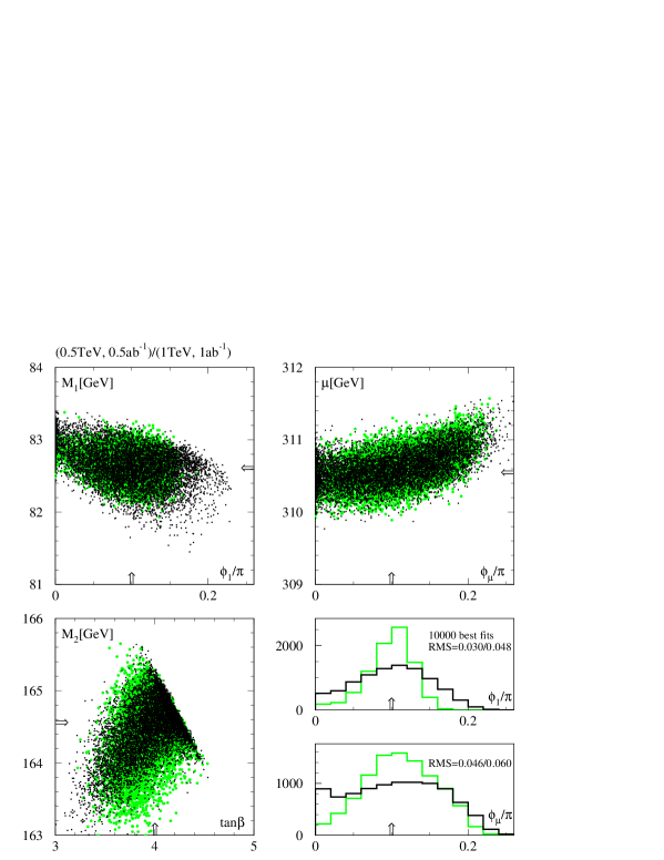
Figure 2.: Parameters obtained from best fits to masses and cross sections with the mSUGRA type parameter choice (1) and $\phi_{1}=0.1\pi$, $\phi_{\mu}=0.1\pi$. All central values are indicated by arrows on the axes. The grey (green) and black points correspond to the low and high performance collider designs, respectively. The straight boundary in the $M_{2}$-$\tan\beta$ plane is an artifact from restricting the phases to $[0,\pi]$; this makes it easier for MINUIT to find a global minimum in $\chi^{2}$.

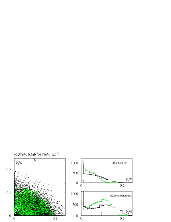
Figure 3.: Parameters obtained from best fits to masses and cross sections with the mSUGRA type parameter choice (2) and $\phi_{1}=0.01\pi$, $\phi_{\mu}=0.1\pi$. The central values are indicated by arrows on the axes. The grey (green) and black points correspond to the low and high performance collider designs, respectively.

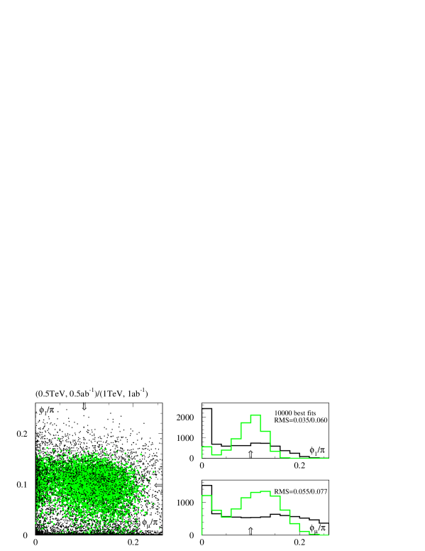
Figure 4.: Parameters obtained from best fits to masses and cross sections at the large $\tan\beta$ mSUGRA parameter point (3) with $\phi_{1}=0.1\pi$, $\phi_{\mu}=0.1\pi$. All central values are indicated by arrows on the axes. The grey (green) and black points correspond to the low and high performance collider designs, respectively.

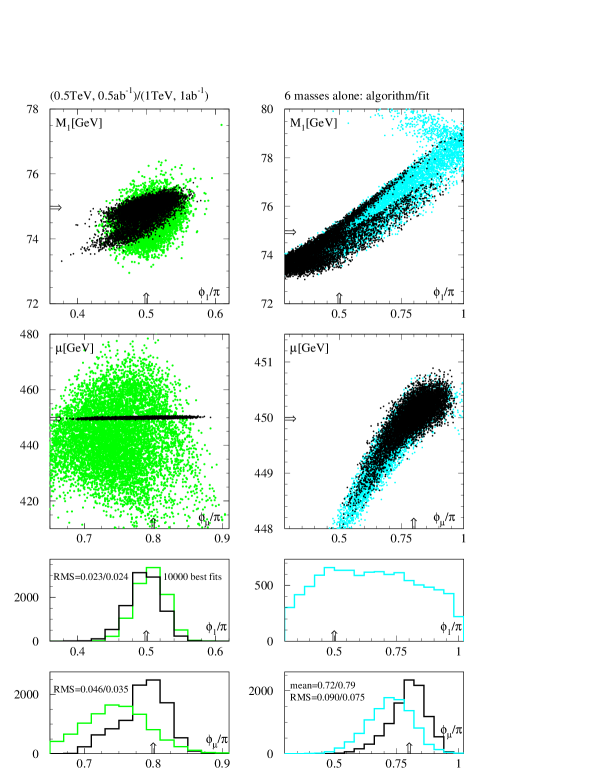
Figure 5.: Parameters obtained from best fits to masses and cross sections (left) and to masses (right) at the large phase parameter point (4) $\phi_{1}=0.5\pi$, $\phi_{\mu}=0.8\pi$. The central values are again indicated by arrows on the axes. The grey (green) and black points correspond to the low and high performance collider designs, respectively. For the grey (blue) dots in the right column of plots the fit to the masses is replaced by the algorithm described in the Appendix.

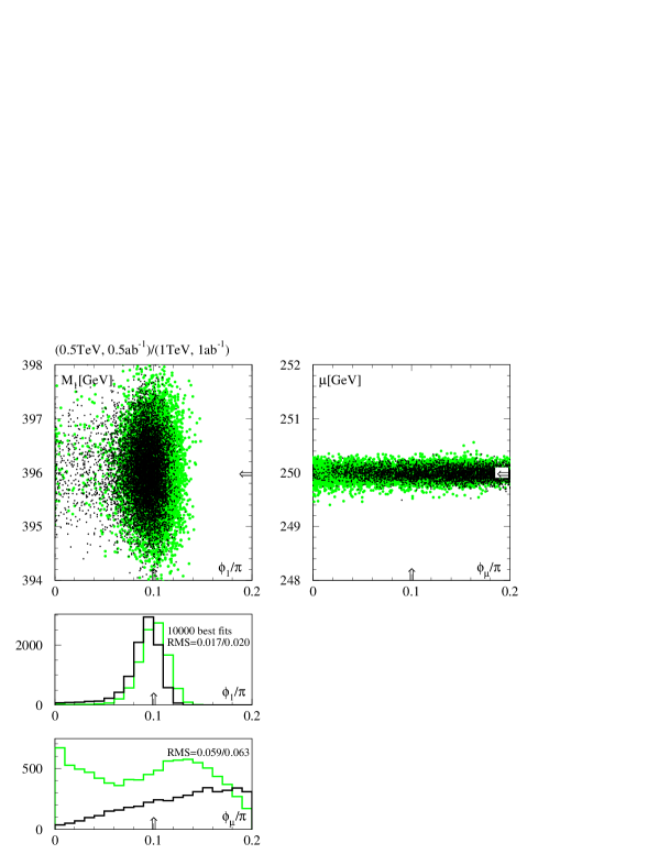
Figure 6.: Parameters obtained from best fits to masses and cross sections at the wino LSP parameter point (5) with $\phi_{1}=0.1\pi$, $\phi_{\mu}=0.1\pi$. The central values are indicated by arrows on the axes. The grey (green) and black points correspond to the low and high performance collider designs, respectively.

Bibliography

- [1] See e.g. H. Nilles, 110 (1984) 1; H.E. Haber and G.L. Kane, 117 (1985) 75; J. Gunion and H.E. Haber, B272 (1986) 1 and Erratum B402 (1993) 567.
- [2] E. Accomando et al. , 299 (1998) 1; G. Blair, http://www.hep.ph.rhbnc.ac.uk/blair/ susy/; H.U. Martyn, International Workshop on Linear Colliders, Sitges, 1999.
- [3] J. Ellis, J. Hagelin, D. Nanopoulos, and M. Srednicki, B127 (1983) 233; V. Barger, R.W. Robinett, W.Y. Keung, and R.J.N. Phillips, B131 (1983) 372; D. Dicus, S. Nandi, W. Repko, and X. Tata, 51 (1983) 1030; S. Dawson, E. Eichten, and C. Quigg, D31 (1985) 1581; A. Bartl and H. Fraas, and W. Majerotto, C30 (1986) 441.
- [4] See e.g. T. Tsukamoto, K. Fujii, H. Murayama, M. Yamaguchi, and Y. Okada D51 (1995) 3153; J.L. Feng, M.E. Peskin, H. Murayama, and X. Tata, D52 (1995) 1418; S.-Y. Choi, A. Djouadi, H. Dreiner, J. Kalinowski, and P.M. Zerwas, C7 (1999) 123; G. Moortgat-Pick, H. Fraas, A. Bartl, and W. Majerotto, C9 (1999) 549.
- [5] M. Dugan, B. Grinstein, and L. Hall, B255 (1985) 413; Y. Kizukuri and N. Oshimo, D45 (1992) 1806; T. Falk, K.A. Olive, and M. Srednicki, B354 (1995) 99.
- [6] T. Falk, K.A. Olive, M. Pospelov, and R. Roiban, 9904393.
- [7] T. Ibrahim and P. Nath, D57 (1998) 478; M. Brhlik, G.J. Good, and G.L. Kane, D59 (1999) 115004.
- [8] S.-Y. Choi, A. Djouadi, H.S. Song, and P.M. Zerwas, C8 (1999) 669.
- [9] J.-L. Kneur and G. Moultaka, 9907360.
- [10] M. Brhlik, private communication.
- [11] L. Randall and R. Sundrum, 9810155.
- [12] G. Moortgat-Pick and H. Fraas, Cracow Epiphany Conf. on Colliders, Cracow, Poland, 1999, 9904209.