hep-ph/9907356
VUTH 99-16
Perspectives in Polarized Leptoproduction

Abstract

We discuss specific observables that can be measured in deep inelastic leptoproduction in the case of 1-particle inclusive measurements, namely azimuthal asymmetries and power-suppressed (higher twist) corrections. These quantities contain information on the intrinsic transverse momentum of partons, with close connection to the gluon dynamics in hadrons.

1 LEPTOPRODUCTION

The use of polarization in leptoproduction in combination with azimuthal sensitivity in the final state provides ways to probe new aspects of hadronic structure. The central object of interest for 1-particle inclusive leptoproduction, the hadronic tensor, is given by

$$2M{\cal W}_{\mu\nu}^{(\ell H)}(q;{PS;P_{h}S_{h}})=\frac{1}{(2\pi)^{4}}\int\frac{d^{3}P_{X}}{(2\pi)^{3}2P_{X}^{0}}(2\pi)^{4}\delta^{4}(q+P-P_{X}-P_{h})$$

$$\hskip 99.58464pt\times\langle{PS}|{J_{\mu}(0)}|P_{X};{P_{h}S_{h}}\rangle\langle P_{X};{P_{h}S_{h}}|{J_{\nu}(0)}|{PS}\rangle,$$ (1)

where $P,\ S$ and $P_{h},\ S_{h}$ are the momenta and spin vectors of target hadron and produced hadron, $q$ is the (spacelike) momentum transfer with $-q^{2}$ = $Q^{2}$ sufficiently large. The kinematics is illustrated in Fig. 1, where also the scaling variables are introduced.

$$\ell H\longrightarrow\ell^{\prime}hX$$

$$x_{{}_{B}}=\frac{Q^{2}}{2P\cdot q}$$

$$y=\frac{P\cdot q}{P\cdot k}$$

$$z_{h}=\frac{P\cdot P_{h}}{P\cdot q}$$

Figure 1: Kinematics for 1-particle inclusive leptoproduction.

Within the framework of QCD, it is possible to write down a diagrammatic expansion with the simplest diagrams being given in Fig. 2 for inclusive and 1-particle inclusive deep inelastic scattering.

1.1 From hadrons to quarks

Figure 2: The simplest (parton-level) diagrams representing the squared amplitude in lepton hadron inclusive scattering (left) and semi-inclusive scattering (right).

In the calculations the relevant structural information for the hadrons is contained in soft parts (the blobs in Fig. 2) which represent specific matrix elements of quark fields. In order to find out which information in the soft parts is important in a hard process one needs to realize that the hard scale $Q$ leads in a natural way to the use of lightlike vectors $n_{+}$ and $n_{-}$ satisfying $n_{+}^{2}=n_{-}^{2}=0$ and $n_{+}\cdot n_{-}$ = 1. For inclusive scattering one parametrizes the momenta

$$\left.\begin{array}[]{l}q^{2}=-Q^{2}\\ P^{2}=M^{2}\\ 2\,P\cdot q=\frac{Q^{2}}{x_{{}_{B}}}\\ \end{array}\right\}\longleftrightarrow\left\{\begin{array}[]{l}q=\frac{Q}{\sqrt{2}}\,n_{-}-\frac{Q}{\sqrt{2}}\,n_{+}+q_{T}\\ \mbox{}\\ P=\frac{x_{{}_{B}}M^{2}}{Q\sqrt{2}}\,n_{-}+\frac{Q}{x_{{}_{B}}\sqrt{2}}\,n_{+}\end{array}\right.$$

The minus component $p^{-}\equiv p\cdot n_{+}$ and transverse components are not relevant in the hard part. The soft part to look at is [1, 2]

$$\Phi_{ij}(x)=\left.\int\frac{d\xi^{-}}{4\pi}\ e^{ip\cdot\xi}\,\langle P,S|\overline{\psi}_{j}(0)\psi_{i}(\xi)|P,S\rangle\right|_{\xi^{+}=\xi_{\scriptstyle T}=0},$$ (2)

where $x=p^{+}/P^{+}$. For the leading order in $1/Q$, it is parametrized as [3]

$$\Phi(x)=\frac{1}{4}\,\Biggl{\{}f_{1}(x)\,\kern 1.99997ptn\kern-3.99994pt/_{+}+\lambda\,g_{1}(x)\,\gamma_{5}\,\kern 1.99997ptn\kern-3.99994pt/_{+}+h_{1}(x)\,\frac{\gamma_{5}\,[\kern 1.99997ptS\kern-5.59998pt\raisebox{1.29167pt}{/}_{\scriptstyle T},\kern 1.99997ptn\kern-3.99994pt/_{+}]}{2}\Biggr{\}}+{\cal O}\left(\frac{M}{P^{+}}\right)$$ (3)

Adding the flavor index $a$, the functions are the unpolarized quark distribution $f_{1}^{a}$, the chirality distribution $g_{1}^{a}$ and the transverse spin distribution $h_{1}^{a}$. For each of these functions there are many aspects to be discussed, such as their interpretation (we will come back to this), positivity and bounds, e.g. $|g_{1}^{a}(x)|\leq f_{1}^{a}(x)$, symmetry relations and antiquark distributions, e.g. $\bar{f}_{1}(x)=-f_{1}(-x)$, sum rules, etc.

For 1-particle inclusive scattering one parametrizes the momenta

$$\left.\begin{array}[]{l}q^{2}=-Q^{2}\\ P^{2}=M^{2}\\ P_{h}^{2}=M_{h}^{2}\\ 2\,P\cdot q=\frac{Q^{2}}{x_{{}_{B}}}\\ 2\,P_{h}\cdot q=-z_{h}\,Q^{2}\end{array}\right\}\longleftrightarrow\left\{\begin{array}[]{l}P_{h}=\frac{z_{h}\,Q}{\sqrt{2}}\,n_{-}+\frac{M_{h}^{2}}{z_{h}\,Q\sqrt{2}}\,n_{+}\\ \mbox{}\\ q=\frac{Q}{\sqrt{2}}\,n_{-}-\frac{Q}{\sqrt{2}}\,n_{+}+q_{T}\\ \mbox{}\\ P=\frac{x_{{}_{B}}M^{2}}{Q\sqrt{2}}\,n_{-}+\frac{Q}{x_{{}_{B}}\sqrt{2}}\,n_{+}\end{array}\right.$$

The minus component $p^{-}$ still is not relevant in the hard part, but the transverse component is. The soft part to look at is

$$\Phi(x,\mbox{\boldmath$p$}_{T})=\left.\int\frac{d\xi^{-}d^{2}\mbox{\boldmath$\xi$}_{T}}{2\,(2\pi)^{3}}\ e^{ip\cdot\xi}\,\langle P,S|\overline{\psi}(0)\psi(\xi)|P,S\rangle\right|_{\xi^{+}=0}.$$ (4)

For the leading order results, it is parametrized as

$$\Phi(x,\mbox{\boldmath$p$}_{\scriptstyle T})=\Phi_{O}(x,\mbox{\boldmath$p$}_{\scriptstyle T})+\Phi_{L}(x,\mbox{\boldmath$p$}_{\scriptstyle T})+\Phi_{T}(x,\mbox{\boldmath$p$}_{\scriptstyle T}),$$ (5)

with the parts involving unpolarized targets (O), longitudinally polarized targets (L) and transversely polarized targets (T) given by

$$\Phi_{O}(x,\mbox{\boldmath$p$}_{\scriptstyle T}) = \frac{1}{4}\Biggl{\{}f_{1}(x,\mbox{\boldmath$p$}_{\scriptstyle T})\,\kern 1.99997ptn\kern-3.99994pt/_{+}+h_{1}^{\perp}(x,\mbox{\boldmath$p$}_{\scriptstyle T})\,\frac{i\,[\kern 1.99997ptp\kern-3.99994pt/_{\scriptstyle T},\kern 1.99997ptn\kern-3.99994pt/_{+}]}{2M}\Biggr{\}}$$

$$\Phi_{L}(x,\mbox{\boldmath$p$}_{\scriptstyle T}) = \frac{1}{4}\Biggl{\{}+\lambda\,g_{1L}(x,\mbox{\boldmath$p$}_{\scriptstyle T})\,\gamma_{5}\,\kern 1.99997ptn\kern-3.99994pt/_{+}+\lambda\,h_{1L}^{\perp}(x,\mbox{\boldmath$p$}_{\scriptstyle T})\Biggr{\}}$$

$$\Phi_{T}(x,\mbox{\boldmath$p$}_{\scriptstyle T}) = \frac{1}{4}\Biggl{\{}+f_{1T}^{\perp}(x,\mbox{\boldmath$p$}_{\scriptstyle T})\,\frac{\epsilon_{\mu\nu\rho\sigma}\gamma^{\mu}n_{+}^{\nu}p_{\scriptstyle T}^{\rho}S_{\scriptstyle T}^{\sigma}}{M}+\frac{\mbox{\boldmath$p$}_{\scriptstyle T}\cdot\mbox{\boldmath$S$}_{\scriptstyle T}}{M}\,g_{1T}(x,\mbox{\boldmath$p$}_{\scriptstyle T})\,\gamma_{5}\,\kern 1.99997ptn\kern-3.99994pt/_{+}$$ (6)

$$\qquad+h_{1T}(x,\mbox{\boldmath$p$}_{\scriptstyle T})\,\frac{\gamma_{5}\,[\kern 1.99997ptS\kern-5.59998pt\raisebox{1.29167pt}{/}_{\scriptstyle T},\kern 1.99997ptn\kern-3.99994pt/_{+}]}{2}+\frac{\mbox{\boldmath$p$}_{\scriptstyle T}\cdot\mbox{\boldmath$S$}_{\scriptstyle T}}{M}\,h_{1T}^{\perp}(x,\mbox{\boldmath$p$}_{\scriptstyle T})\,\frac{\gamma_{5}\,[\kern 1.99997ptp\kern-3.99994pt/_{\scriptstyle T},\kern 1.99997ptn\kern-3.99994pt/_{+}]}{2M}\Biggr{\}}.$$

Again all functions appearing here have a natural interpretation as densities, now including densities such as the density of longitudinally polarized quarks in a transversely polarized nucleon ($g_{1T}$) and the density of transversely polarized quarks in a longitudinally polarized nucleon ($h_{1L}^{\perp}$). These functions vanish from the soft part upon integration over $p_{\scriptstyle T}$. Actually we will find that particularly interesting functions to consider are

$$g_{1T}^{(1)}(x)=\int d^{2}p_{\scriptstyle T}\ \frac{\mbox{\boldmath$p$}_{\scriptstyle T}^{2}}{2M^{2}}\,g_{1T}(x,\mbox{\boldmath$p$}_{\scriptstyle T}),$$ (7)

and similarly the function $h_{1L}^{\perp(1)}$. The functions $h_{1}^{\perp}$ and $f_{1T}^{\perp}$ are T-odd, vanishing if T-reversal invariance can be applied to the matrix element. For $k_{\scriptstyle T}$-dependent correlation functions, matrix elements involving gluonic fields at infinity (gluonic poles [4]) can for instance prevent application of T-reversal invariance. The functions describe the possible appearance of unpolarized quarks in a transversely polarized nucleon ($f_{1T}^{\perp}$) or transversely polarized quarks in an unpolarized hadron ($h_{1}^{\perp}$) and lead to single-spin asymmetries in various processes [5, 6]. The interpretation of the functions is illustrated in Fig. 3.

Figure 3: Interpretation of the functions in the leading Dirac projections of $\Phi$.

If one proceeds up to order $1/Q$ one also needs to include in the parametrization of the soft part the parts proportional to $M/P^{+}$ and account for gluonic diagrams. For the $\mbox{\boldmath$k$}_{\scriptstyle T}$-integrated correlations one has

$$\Phi(x) = \frac{1}{4}\,\Biggl{\{}f_{1}(x)\,\kern 1.99997ptn\kern-3.99994pt/_{+}+\lambda\,g_{1}(x)\,\gamma_{5}\,\kern 1.99997ptn\kern-3.99994pt/_{+}+h_{1}(x)\,\frac{\gamma_{5}\,[\kern 1.99997ptS\kern-5.59998pt\raisebox{1.29167pt}{/}_{\scriptstyle T},\kern 1.99997ptn\kern-3.99994pt/_{+}]}{2}\Biggr{\}}$$ (8)

$$+\frac{M}{4P^{+}}\Biggl{\{}e(x)+g_{T}(x)\,\gamma_{5}\,\kern 1.99997ptS\kern-5.59998pt\raisebox{1.29167pt}{/}_{\scriptstyle T}+\lambda\,h_{L}(x)\,\frac{\gamma_{5}\,[\kern 1.99997ptn\kern-3.99994pt/_{+},\kern 1.99997ptn\kern-3.99994pt/_{-}]}{2}\Biggr{\}}$$

$$+\frac{M}{4P^{+}}\Biggl{\{}-\lambda\,e_{L}(x)\,i\gamma_{5}-f_{T}(x)\,\epsilon_{\scriptstyle T}^{\rho\sigma}\gamma_{\rho}S_{{\scriptstyle T}\sigma}+h(x)\,\frac{i\,[\kern 1.99997ptn\kern-3.99994pt/_{+},\kern 1.99997ptn\kern-3.99994pt/_{-}]}{2}\Biggr{\}}.$$

Actually gluonic diagrams (what is needed are matrix elements containing $\overline{\psi}(0)\,A_{\scriptstyle T}^{\alpha}(\xi)\,\psi(\xi)$) do not give rise to new functions, but they can be related to the above subleading result using the QCD equations of motion. It is important, however, to include gluonic contributions in order to obtain a gauge invariant result.

From Lorentz invariance one obtains, furthermore, some interesting relations between the subleading functions and the $k_{\scriptstyle T}$-dependent leading functions [7, 8, 9]

$$g_{T}=g_{1}+\frac{d}{dx}\,g_{1T}^{(1)},$$ (9)

$$h_{L}=h_{1}-\frac{d}{dx}\,h_{1L}^{\perp(1)},$$ (10)

$$f_{T}=-\frac{d}{dx}\,f_{1T}^{\perp(1)},$$ (11)

$$h=-\frac{d}{dx}\,h_{1}^{\perp(1)}.$$ (12)

1.2 From quarks to hadrons

Just as for the distribution functions one can perform an analysis of the soft part describing the quark fragmentation. One needs [10]

$$\Delta_{ij}(z,{\mbox{\boldmath$k$}}_{{}_{T}})=\left.\sum_{X}\int\frac{d\xi^{+}d^{2}\mbox{\boldmath$\xi$}_{\scriptstyle T}}{4z\,(2\pi)^{3}}\,e^{ik\cdot\xi}\,Tr\langle 0|\psi_{i}(\xi)|P_{h},X\rangle\langle P_{h},X|\overline{\psi}_{j}(0)|0\rangle\right|_{\xi^{-}=0}.$$ (13)

For the production of unpolarized hadrons $h$ one needs in leading order in $1/Q$ in hard processes [8]

$$\Delta(z,\mbox{\boldmath$k$}_{\scriptstyle T})=\frac{1}{4}\Biggl{\{}D_{1}(z,\mbox{\boldmath$k$}^{\prime}_{\scriptstyle T})\,\kern 1.99997ptn\kern-3.99994pt/_{-}+H_{1}^{\perp}(z,\mbox{\boldmath$k$}^{\prime}_{\scriptstyle T})\,\frac{i\,[\kern 1.99997ptk\kern-4.49997pt/_{\scriptstyle T},\kern 1.99997ptn\kern-3.99994pt/_{-}]}{2M_{h}}\Biggr{\}}+{\cal O}\left(\frac{M_{h}}{P_{h}^{-}}\right).$$ (14)

The arguments of the fragmentation functions $D_{1}$ and $H_{1}^{\perp}$ are chosen to be $z$ = $P_{h}^{-}/k^{-}$ and $\mbox{\boldmath$k$}^{\prime}_{\scriptstyle T}$ = $-z{\mbox{\boldmath$k$}}_{{}_{T}}$. The first is the (lightcone) momentum fraction of the produced hadron, the second is the transverse momentum of the produced hadron with respect to the quark. The fragmentation function $D_{1}$ is the equivalent of the distribution function $f_{1}$. It can be interpreted as the probability of finding a hadron $h$ in a quark. The function $H_{1}^{\perp}$, interpretable as the difference in production probabilities of unpolarized hadrons from a transversely polarized quark depending on transverse momentum, is allowed because of the non-applicability of time reversal invariance. This is natural for the fragmentation functions because of the appearance of out-states $|P_{h},X\rangle$ in the definition of $\Delta$, in contrast to the plane wave states appearing in $\Phi$. After ${\mbox{\boldmath$k$}}_{{}_{T}}$-averaging one is left with the functions $D_{1}(z)$ and the ${\mbox{\boldmath$k$}}_{{}_{T}}/M$-weighted result $H_{1}^{\perp(1)}(z)$. As in the case of distribution functions, the latter function can be related to a function $H(z)$, appearing at subleading order,

$$\frac{H(z)}{z}=z^{2}\,\frac{d}{dz}\left(\frac{H_{1}^{\perp}}{z}\right).$$ (15)

2 CROSS SECTIONS FOR LEPTOPRODUCTION

After the analysis of the soft parts, the next step is to find out how one obtains the information on the various correlation functions from experiments, in this particular case in lepton-hadron scattering via one-photon exchange as discussed before. To get the leading order result for semi-inclusive scattering it is sufficient to compute the diagram in Fig. 2 (right) by using QCD and QED Feynman rules in the hard part and the matrix elements $\Phi$ and $\Delta$ for the soft parts, parametrized in terms of distribution and fragmentation functions. The most well-known results for leptoproduction are:

Cross sections (leading in $1/Q$) $\displaystyle\frac{d\sigma_{OO}}{dx_{{}_{B}}\,dy\,dz_{h}}=\frac{2\pi\alpha^{2}\,s}{Q^{4}}\,\sum_{a,\bar{a}}e_{a}^{2}\left\lgroup 1+(1-y)^{2}\right\rgroup x_{{}_{B}}{f^{a}_{1}}(x_{{}_{B}})\,{D^{a}_{1}}(z_{h})$ (16) $\displaystyle\frac{d\sigma_{LL}}{dx_{{}_{B}}\,dy\,dz_{h}}=\frac{2\pi\alpha^{2}\,s}{Q^{4}}\,{\lambda_{e}\,\lambda}\,\sum_{a,\bar{a}}e_{a}^{2}\ y(2-y)\ x_{{}_{B}}{g^{a}_{1}}(x_{{}_{B}})\,{D^{a}_{1}}(z_{h})$ (17)

The indices attached to the cross section refer to polarization of lepton (O is unpolarized, L is longitudinally polarized) and hadron (O is unpolarized, L is longitudinally polarized, T is transversely polarized). Note that the result is a weighted sum over quarks and antiquarks involving the charge $e_{a}$ squared. Comparing with well-known formal expansions of the cross section in terms of structure functions one can simply identify these. For instance the above result for unpolarized scattering (OO) shows that after averaging over azimuthal angles, only one structure function survives if we work at order $\alpha_{s}^{0}$ and at leading order in $1/Q$.

It is well-known that in 1-particle inclusive unpolarized leptoproduction in principle four structures appear, two of them containing azimuthal dependence of the form $\cos(\phi_{h}^{\ell})$ and $\cos(2\phi_{h}^{\ell})$. The first one only appears at order $1/Q$ [11], the second one even at leading order but only in the case of the existence of nonvanishing T-odd distribution functions. To be specific if we define weighted cross section such as

$$\int d^{2}\mbox{\boldmath$q$}_{T}\,\frac{Q_{T}^{2}}{MM_{h}}\,\cos(2\phi_{h}^{\ell})\,\frac{d\sigma_{{OO}}}{dx_{{}_{B}}\,dy\,dz_{h}\,d^{2}\mbox{\boldmath$q$}_{T}}\equiv\left<\frac{Q_{T}^{2}}{MM_{h}}\,\cos(2\phi_{h}^{\ell})\right>_{OO}$$ (18)

we obtain the following asymmetry.
Azimuthal asymmetries for unpolarized targets (leading twist) $$\left<\frac{Q_{T}^{2}}{MM_{h}}\,\cos(2\phi_{h}^{\ell})\right>_{OO}=\frac{16\pi\alpha^{2}\,s}{Q^{4}}\,(1-y)\,\sum_{a,\bar{a}}e_{a}^{2}\,x_{{}_{B}}\,{h_{1}^{\perp(1)a}}(x_{{}_{B}})H_{1}^{\perp(1)a}.$$ (19)

An interesting asymmetry involving the same fragmentation part is a $\sin(\phi_{h}^{\ell})$ single spin asymmetry, requiring only a polarized lepton but no polarization for the target [11].

Single spin asymmetry for unpolarized targets (higher twist) $\displaystyle\left<\frac{Q_{T}}{M}\,\sin(\phi_{h}^{\ell})\right>_{LO}=\frac{4\pi\alpha^{2}\,s}{Q^{4}}\,{\lambda_{e}}\,y\sqrt{1-y}\,\frac{2M}{Q}\,x_{{}_{B}}^{2}{\tilde{e}^{a}}(x_{{}_{B}})\,{H_{1}^{\perp(1)a}}(z_{h})$ (20) $\displaystyle\mbox{note:}\ {\tilde{e}^{a}}(x)=e^{a}(x)-\frac{m_{a}}{M}\,\frac{f_{1}^{a}(x)}{x}.$

This cross section involves, besides the time-reversal odd fragmentation function $H_{1}^{\perp}$, the distribution function $e$. The tilde function that appear in the cross sections is in fact the socalled interaction dependent part of the twist three functions. It would vanish in any naive parton model calculation in which cross sections are obtained by folding electron-parton cross sections with parton densities. Considering the relation for $\tilde{e}$ one can state it as $x\,e(x)$ = $(m/M)\,f_{1}(x)$ in the absence of quark-quark-gluon correlations. The inclusion of the latter also requires diagrams dressed with gluons.

For polarized targets, several azimuthal asymmetries arise already at leading order. For example the following possibilities were investigated in Refs [12, 13, 14, 15].

Azimuthal asymmetries for polarized targets (leading twist) $\displaystyle\left<\frac{Q_{\scriptstyle T}}{M}\,\cos(\phi_{h}^{\ell}-\phi_{S}^{\ell})\right>_{LT}=\frac{2\pi\alpha^{2}\,s}{Q^{4}}\,{\lambda_{e}\,|{\mbox{\boldmath$S$}}_{{}_{T}}|}\,y(2-y)\sum_{a,\bar{a}}e_{a}^{2}\,x_{{}_{B}}\,{g_{1T}^{(1)a}}(x_{{}_{B}}){D^{a}_{1}}(z_{h}),$ (21) $\displaystyle\left<\frac{Q_{\scriptstyle T}^{2}}{MM_{h}}\,\sin(2\phi_{h}^{\ell})\right>_{OL}=-\frac{4\pi\alpha^{2}\,s}{Q^{4}}\,{\lambda}\,(1-y)\sum_{a,\bar{a}}e_{a}^{2}\,x_{{}_{B}}\,{h_{1L}^{\perp(1)a}}(x_{{}_{B}}){H_{1}^{\perp(1)a}}(z_{h}),$ (22) $\displaystyle\left<\frac{Q_{\scriptstyle T}}{M_{h}}\,\sin(\phi_{h}^{\ell}+\phi_{S}^{\ell})\right>_{OT}=\frac{4\pi\alpha^{2}\,s}{Q^{4}}\,{|{\mbox{\boldmath$S$}}_{{}_{T}}|}\,(1-y)\sum_{a,\bar{a}}e_{a}^{2}\,x_{{}_{B}}\,{h_{1}^{a}}(x_{{}_{B}}){H_{1}^{\perp(1)a}}(z_{h}).$ (23)

The latter two are single spin asymmetries involving the fragmentation function $H_{1}^{\perp(1)}$. The last one was the asymmetry proposed by Collins [13] as a way to access the transverse spin distribution function $h_{1}$ in pion production. Note, however, that in using the azimuthal dependence one needs to be very careful. For instance, besides the $<\sin(\phi_{h}^{\ell}+\phi_{S}^{\ell})>_{OT}$, one also finds at leading order a $<\sin(3\phi_{h}^{\ell}-\phi_{S}^{\ell})>_{OT}$ asymmetry which is proportional to $h_{1T}^{\perp(2)}\,H_{1}^{\perp(1)}$ [15].

Notice that an estimate of the function $g_{1T}^{(1)}$ can be obtained from inclusive results for $g_{2}$ using the relation 9 for $g_{T}=g_{1}+g_{2}$. Actually this relation is exact and the data from the SLAC E143 experiment were used for an estimate in Ref. [12]. An update using the preliminary $g_{2}$ data from the E155 experiment is shown in Fig. 5. More about the final analysis of these data will be reported in Ref. [16]. A well-known approximation for $g_{2}$ is the Wandzura-Wilczek result [17]. An alternative derivation of this relation is obtained by combining the separation of the twist three function $g_{T}$ into a twist-two part and an interaction dependent part $\tilde{g}_{T}$, omitting quark mass terms given by

$$g_{T}(x)=\frac{g_{1T}^{(1)}(x)}{x}+\tilde{g}_{T}(x).$$ (24)

By eliminating $g_{1T}^{(1)}$ one then derives the relation

$$g_{T}(x)=\int_{x}^{1}dy\,\frac{g_{1}(y)}{y}+\underbrace{\left(\tilde{g}_{T}(x)-\int_{x}^{1}dy\,\frac{\tilde{g}_{T}(y)}{y}\right)}_{\bar{g}_{T}(x)}.$$ (25)

The Wandzura-Wilczek part is obtained by putting $\bar{g}_{T}(x)=0$. Within this approximation one can find an estimate for $g_{1T}^{(1)}$ from the $g_{1}$-data, the result of which using the SMC data [18] is shown in Fig. 5.

Figure 4: An estimate for the function $g_{1T}^{(1)}(x)$ using $g_{2}$-data and the Wandzura-Wilczek approximation obtained from the SMC $g_{1}$-data.

Figure 5: An estimate for the function $h_{1L}^{\perp(1)}(x)$ obtained from $h_{1}$ using a ’Wandzura-Wilczek’-like approximation.

In the same experiment in which one would measure the single spin asymmetry $<\sin(\phi_{h}^{\ell}+\phi_{S}^{\ell})>_{OT}$, one can also measure the possible existence of a $<\sin(\phi_{h}^{\ell}-\phi_{S}^{\ell})>_{OT}$ asymmetry. Such an asymmetry would arise from a T-odd distribution function; to be precise
$$\left<\frac{Q_{T}}{M_{h}}\,\sin(\phi^{\ell}_{h}-\phi^{\ell}_{S})\right>_{OTO}=\frac{2\pi\alpha^{2}\,s}{Q^{4}}\,|\mbox{\boldmath$S$}_{T}|\,\left(1-y-\frac{1}{2}\,y^{2}\right)\sum_{a,\bar{a}}e_{a}^{2}\,x_{{}_{B}}\,f_{1T}^{\perp(1)a}(x_{{}_{B}})D_{1}^{a}(z_{h}).$$ (26)

By comparing the results for 23 and 26, leptoproduction could resolve an ambiguity in the explanation of the single spin (left-right) asymmetry observed in $p^{\uparrow}p\rightarrow\pi X$, which can be attributed to a T-odd effect in the initial state (Sivers effect, $f_{1T}^{\perp(1)}$ [5, 6]) or a T-odd effect in the final state (Collins effect, $H_{1}^{\perp(1)}$ [19]). Estimates for the leptoproduction asymmetries for both cases have been presented in Ref. [20] and are found to have quite characteristic behavior as a function of $x_{{}_{B}}$ and $z_{h}$.

As a final example, we want to concentrate on single spin asymmetries $<\sin(\phi_{h}^{\ell})>_{LO}$, $<\sin(\phi_{h}^{\ell})>_{OL}$ and $<\sin(2\phi_{h}^{\ell})>_{OL}$, for which preliminary results have been presented [21] by the HERMES collaboration. The results for two of these have been mentioned already (Eqs 20 and 22), the other one is actually a higher twist result [8],
$\displaystyle\left<\frac{Q_{T}}{M_{h}}\,\sin(\phi^{\ell}_{h})\right>_{OL}=\frac{4\pi\alpha^{2}\,s}{Q^{4}}\,\lambda\,(2-y)\sqrt{1-y}\,\sum_{a,\bar{a}}e_{a}^{2}\,\Biggl{\{}x_{{}_{B}}\,h_{1L}^{\perp(1)a}(x_{{}_{B}})\frac{\tilde{H}^{a}(z_{h})}{z_{h}}$ $\displaystyle\mbox{}\hskip 156.49014pt+x_{{}_{B}}\left(2\,h_{1L}^{\perp(1)a}(x_{{}_{B}})-x_{{}_{B}}\,\tilde{h}_{L}^{a}(x_{{}_{B}})\right)H_{1}^{\perp(1)a}(z_{h})\Biggr{\}}.$ (27)

In the same way as discussed for $g_{T}$ and $g_{1T}^{(1)}$, we also have relations between the $h$-functions. One can combine the decomposition of the function $h_{L}$, appearing at subleading order in leptoproduction, into a twist-two part and an interaction dependent part (omitting quark mass dependent terms),

$$h_{L}(x)=-2\,\frac{h_{1L}^{\perp(1)}(x)}{x}+\tilde{h}_{L}(x),$$ (28)

with Eq. 10 to eliminate $h_{1L}^{\perp(1)}$ and find

$$h_{L}(x)=2x\int_{x}^{1}dy\,\frac{h_{1}(y)}{y^{2}}+\underbrace{\left(\tilde{h}_{L}(x)-2x\int_{x}^{1}dy\,\frac{\tilde{h}_{L}(y)}{y^{2}}\right)}_{\bar{h}_{L}}.$$ (29)

The approximation $\bar{h}_{L}=0$ e.g. can be used to obtain an idea of the magnitude of $h_{L}$ and then with the exact Eq. 10 an estimate for $h_{1L}^{\perp(1)}$. One needs as input some reasonable guess for $h_{1}$ (e.g. in our case we took $h_{1}$ = $f_{1}$ up to some spin factors) to get the estimate in Fig. 5. We find that the functions $g_{1T}^{(1)}$ and $h_{1L}^{\perp(1)}$ are of the same order of magnitude, and about an order of magnitude smaller than the functions $f_{1}$ and $g_{1}$. With the presented estimates and the estimate for $H_{1}^{\perp(1)}$ from Ref. [19] which not only determines the functions $H$ (Eq. 15) but also $\tilde{H}$,

$$H(z)=-2z\,H_{1}^{\perp(1)}(z)+\tilde{H}(z),$$ (30)

we find for the single spin asymmetries the results in Figs 7 and 7. Note that the $<\sin(\phi_{h}^{\ell})>_{OL}$ asymmetry is larger than the $<\sin(2\phi_{h}^{\ell})>_{OL}$ asymmetry. This shows e.g. that the absence in the HERMES results of a clear signal for the second asymmetry does not allow conclusions on the magnitude of $h_{1L}^{\perp(1)}$.

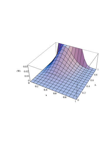
Figure 6: An estimate for the asymmetry $<\sin(\phi_{h}^{\ell})>_{OL}$ (see text). We only plotted the weighted product of distribution and fragmentation functions omitting the $y$-dependence.

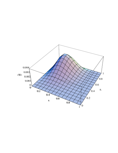
Figure 7: An estimate for the asymmetry $<\sin(2\phi_{h}^{\ell})>_{OL}$ (see text). We only plotted the weighted product of distribution and fragmentation functions omitting the $y$-dependence.

3 CONCLUDING REMARKS

In the previous section some results for 1-particle inclusive lepton-hadron scattering have been presented. Several other effects are important in these cross sections, such as target fragmentation, the inclusion of gluons in the calculation to obtain color-gauge invariant definitions of the correlation functions and an electromagnetically gauge invariant result at order $1/Q$, and finally QCD corrections which can be moved back and forth between hard and soft parts, leading to the scale dependence of the soft parts and the DGLAP equations.

In this contribution we have tried to indicate why semi-inclusive, in particular 1-particle inclusive lepton-hadron scattering, can be important. The goal is the study of the quark and gluon structure of hadrons, emphasizing the dependence on transverse momenta of quarks. The reason why this prospect is promising is the existence of a field theoretical framework that allows a clean study involving well-defined hadronic matrix elements. It does require, however, also a dedicated experimental effort using polarized beams, targets and detection of final state hadrons.

References

• [1] D.E. Soper, Phys. Rev. D 15 (1977) 1141; Phys. Rev. Lett. 43 (1979) 1847.
• [2] R.L. Jaffe, Nucl. Phys. B 229 (1983) 205.
• [3] R.L. Jaffe and X. Ji, Nucl. Phys. B 375 (1992) 527.
• [4] N. Hammon, O. Teryaev and A. SchΓ€fer, Phys. Lett. B390 (1997) 409; D. Boer, P.J. Mulders and O.V. Teryaev, Phys. Rev. D57 (1998) 3057.
• [5] D. Sivers, Phys. Rev. D41 (1990) 83 and Phys. Rev. D43 (1991) 261 and
• [6] M. Anselmino, M. Boglione and F. Murgia, Phys. Lett. B362 (1995) 164; M. Anselmino and F. Murgia, Phys. Lett. B442 (1998) 470.
• [7] A.P. Bukhvostov, E.A. Kuraev and L.N. Lipatov, Sov. Phys. JETP 60 (1984) 22.
• [8] R.D. Tangerman and P.J. Mulders, Nucl. Phys. B461 (1996) 197.
• [9] D. Boer and P.J. Mulders, Phys. Rev. D 57 (1998) 5780.
• [10] J.C. Collins and D.E. Soper, Nucl. Phys. B 194 (1982) 445.
• [11] J. Levelt and P.J. Mulders, Phys. Rev. D 49 (1994) 96; Phys. Lett. B 338 (1994) 357.
• [12] A. Kotzinian and P.J. Mulders, Phys. Rev. D54 (1996) 1229.
• [13] J. Collins, Nucl. Phys. B396 (1993) 161.
• [14] A. Kotzinian, Nucl. Phys. B 441 (1995) 234.
• [15] R.D. Tangerman and P.J. Mulders, Phys. Lett. B352 (1995) 129.
• [16] See P.E. Bosted contribution in this proceedings.
• [17] S. Wandzura and F. Wilczek, Phys. Rev. D16 (1977) 707.
• [18] D. Adams et al., Phys. Rev. D56 (1997) 5330.
• [19] M. Anselmino, M. Boglione, F. Murgia, hep-ph/9901442, to be publ. in Phys. Rev. D.
• [20] M. Boglione and P.J. Mulders, hep-ph/9903354, to be publ. in Phys. Rev. D
• [21] K. Oganessian, to be published in the proceedings of DIS 99, Zeuthen, April 19-23, 1999. See also H. Avakian contribution in this proceedings.