Abstract

We consider a minimal extension to higher dimensions of the Standard Model, having one compactified dimension, and we study its experimental tests in terms of electroweak data. We discuss tests from high-energy data at the $Z$-pole, and low-energy tests, notably from atomic parity violation data. This measurement combined with neutrino scattering data strongly restricts the allowed region of the model parameters. Furthermore this region is incompatible at 95% CL with the restrictions from high-energy experiments. Of course a global fit to all data is possible but the $\chi^{2}_{\rm min}$ for degree of freedom is unpleasantly large.

1 Introduction

Since the original proposal by Kaluza [1] and by Klein [2] the possibility of compactified extra dimensions has been a recurrent theme in theoretical physics, in particular in supergravity and string theories. Recent developments have suggested the possibility of low compactification scales [3, 4]. There have also been similar developments on extensions of the Standard Model (SM) to include compactified extra spatial dimensions [5]. A simplest minimal extension is to 5 dimensions, leading to towers of Kaluza-Klein (KK) excitations of the SM gauge bosons. Within such an extension, precision electroweak measurements have been analyzed to derive bounds on the compactification scale [6, 7].

In this note we present a new discussion of these tests, analyzing the roles played by precision high-energy measurements at the $Z$-pole, as summarized in the $\epsilon$ parameters [8] (or $S$, $T$, $U$ parameters [9]), and by low-energy experiments, in particular the new experiment on the weak charge $Q_{W}$ in atomic cesium [10], whose implications for various models have already been analyzed in [11]. The reason why we have chosen to describe the high-energy measurements in terms of the $\epsilon$’s is that they are just an efficient way of collecting all the relevant data about the observables and also because they can be expressed easily in analytical way. This can be done by eliminating the KK excitations and constructing an effective lagrangian around the $Z$-pole and an effective four-fermi interaction (eliminating also the $W$ and the $Z$) in the low-energy limit $E<<m_{Z}$. This allows us also to perform a simple discussion of the low-energy observables.

In this paper we are mainly interested in studying the compatibility of the model with all the available data. This is done by considering separately the effects of the different measurements on the parameter space. The reason why we choose this procedure is because the low-energy experiments test phenomenological aspects which cannot be tested from measurements at the $Z$-pole. The low-energy experiments provide for measurements of the effective electroweak coupling of the light quarks and leptons, which in ”new physics” schemes might not be directly related to the studies done at the $Z$-pole.

In particular we have performed a fit to the high-energy data, by obtaining bounds on the compactification scale in terms of the mixing of the KK excitations with the $Z$. These data alone leave room to the new physics described here, in fact the $\chi^{2}_{\rm min}$/d.o.f. of the fit turns out to be acceptable. On the other hand the low-energy data leave almost no space to the model. This is mainly due to the new data on Atomic Parity Violation (APV) which put a lower limit on the mixing angle $\beta$ of this model allowing only the region around the maximal mixing. In fact the new results on APV, if taken literally, disfavor the SM and all the models giving rise to negative extra contributions to $Q_{W}$ at more than 99% CL. In the maximal mixing region, where the extra contribution to $Q_{W}$ turns out to be positive, the neutrino scattering experiments as NuTeV and CHARM cut off most of the region allowed by $Q_{W}$. Furthermore, the regions allowed by $Q_{W}$ and by the high-energy data result to be incompatible at 95% CL.

One could also combine all the previous data obtaining bounds on the parameter space. We have tried to do this by putting together the high-energy data with the $Q_{W}$ measurement. The result is that, although the allowed region is not very much dissimilar to the one obtained using only the high-energy data, the $\chi^{2}_{\rm min}$/d.o.f. deteriorates in a considerable way.

In Section 2 we present the effective lagrangian obtained after eliminating the KK modes. This lagrangian is useful to describe physics at energies much lower than the compactification scale, as for $E\approx m_{Z}$. In Sections 3 and 4 we discuss the bounds from the high-energy and the low-energy data respectively. Conclusions are given in Section 5.

2 An extension of the SM in 5 dimensions

The extra dimension model we consider, is the one suggested by [5] and it is based on an extension of the SM to 5 dimensions. The fifth dimension $x^{5}$ is compactified on a circle of radius $R$ with the identification $x^{5}\to-x^{5}$ ($Z_{2}$-parity). Gauge fields and one Higgs field ($\phi_{1}$) live in the bulk, fermions and a second Higgs field $\phi_{2}$ live on the 4D wall (boundary). The action for the SM with one extra dimension is obtained from the action for the general 5D gauge theory. The fields living in the bulk are defined to be even under the $Z_{2}$-parity. In the case of an $SU(2)_{L}\otimes U(1)$ gauge group, integrating over the fifth dimension, the resulting 4D theory (in the unitary gauge) is given by (omitting the kinetic terms):

$${\cal L}^{charged} = \frac{1}{8}\tilde{g}^{2}v^{2}\Big{[}W_{1}^{2}+c_{\beta}^{2}\sum_{n=1}^{\infty}(W_{1}^{(n)})^{2}+2\sqrt{2}s_{\beta}^{2}W_{1}\sum_{n=1}^{\infty}W_{1}^{(n)}$$ (1)

$$+ 2s_{\beta}^{2}(\sum_{n=1}^{\infty}W_{1}^{(n)})^{2}\Big{]}+\frac{1}{2}\sum_{n=1}^{\infty}n^{2}M^{2}(W_{1}^{(n)})^{2}$$

$$- \tilde{g}(W_{1}^{\mu}+\sqrt{2}\sum_{n=1}^{\infty}W_{1}^{(n)\mu})J_{\mu}^{1}+(1\to 2)$$

$${\cal L}^{neutral} = \frac{1}{8}\frac{\tilde{g}^{2}}{{\tilde{c}}_{\theta}^{2}}v^{2}\Big{[}Z^{2}+c_{\beta}^{2}\sum_{n=1}^{\infty}(Z^{(n)})^{2}+2\sqrt{2}s_{\beta}^{2}Z\sum_{n=1}^{\infty}Z^{(n)}$$ (2)

$$+ 2s_{\beta}^{2}(\sum_{n=1}^{\infty}Z^{(n)})^{2}\Big{]}+\frac{1}{2}\sum_{n=1}^{\infty}n^{2}M^{2}[(Z^{(n)})^{2}+(A^{(n)})^{2}]$$

$$- \frac{\tilde{e}}{{\tilde{s}}_{\theta}{\tilde{c}}_{\theta}}(Z^{\mu}+\sqrt{2}\sum_{n=1}^{\infty}Z^{(n)\mu})J_{\mu}^{Z}-{\tilde{e}}(A^{\mu}+\sqrt{2}\sum_{n=1}^{\infty}A^{(n)\mu})J^{em}_{\mu}$$

where $M=1/R$, $\tilde{g}$ and $\tilde{g}^{\prime}$ are the gauge couplings and $\tan\tilde{\theta}={\tilde{s}}_{\theta}/{\tilde{c}}_{\theta}=\tilde{g}^{\prime}/\tilde{g}$, $\tilde{e}=\tilde{g}{\tilde{s}}_{\theta}$. $W^{(n)}$, $Z^{(n)}$ and $A^{(n)}$ are the KK excitations of the standard $W$, $Z$ and $A$ fields, $<\phi_{1}>=v\cos\beta\equiv vc_{\beta}$, $<\phi_{2}>=v\sin\beta\equiv vs_{\beta}$, and

$$J_{\mu}^{1,2} = \bar{\psi}_{L}\gamma_{\mu}\frac{\tau_{1,2}}{2}\psi_{L}$$

$$J_{\mu}^{Z} = \bar{\psi}\gamma_{\mu}(g_{v}+\gamma_{5}g_{a})\psi,~{}~{}~{}~{}g_{v}=\frac{T_{3L}}{2}-{\tilde{s}}_{\theta}^{2}Q,~{}~{}~{}~{}g_{a}=-\frac{T_{3L}}{2}$$

$$J_{\mu}^{em} = \bar{\psi}\gamma_{\mu}Q\psi,~{}~{}~{}~{}Q=T_{3L}+\frac{B-L}{2}$$ (3)

The effects of the KK excitations in the low-energy limit $p^{2}<<M^{2}$, can be studied by eliminating the corresponding fields using the solutions of their equations of motion for $M\to\infty$ [12]. In this limit the kinetic terms are negligible and one gets:

$$W^{(n)}_{1,2} \sim -\sqrt{2}\frac{s_{\beta}^{2}}{n^{2}}\frac{{\tilde{m}}^{2}_{W}}{M^{2}}W_{1,2}+\sqrt{2}\frac{\tilde{g}}{n^{2}M^{2}}J^{1,2}$$

$$Z^{(n)} \sim -\sqrt{2}\frac{s_{\beta}^{2}}{n^{2}}\frac{{\tilde{m}}^{2}_{Z}}{M^{2}}Z+\sqrt{2}\frac{\tilde{e}}{{\tilde{s}}_{\theta}{\tilde{c}}_{\theta}}\frac{1}{n^{2}M^{2}}J^{Z}$$

$$A^{(n)} \sim \sqrt{2}\frac{\tilde{e}}{n^{2}M^{2}}J^{em}$$ (4)

where ${\tilde{m}}^{2}_{W}=\tilde{g}^{2}v^{2}/4$ and ${\tilde{m}}^{2}_{Z}={\tilde{m}}^{2}_{W}/{\tilde{c}}_{\theta}^{2}$. We use tilded quantities to indicate that, due to the effects of the KK excitations, they are not the physical parameters. We do not use tilded notations for the fields because they are not renormalized at the order ${\cal O}(1/M^{2})$.

By using eq. (4) in eqs. (1) and (2), one can read the mass values for $W$ and $Z$ (to order ${\cal O}(1/M^{2})$)

$$m^{2}_{W}={\tilde{m}}_{W}^{2}[1-{\tilde{c}}_{\theta}^{2}s_{\beta}^{4}X],~{}~{}~{}~{}m^{2}_{Z}={\tilde{m}}_{Z}^{2}[1-s_{\beta}^{4}X]$$ (5)

where

$$X=\frac{\pi^{2}}{3}\frac{m_{Z}^{2}}{M^{2}}$$ (6)

The effective couplings are given by

$${\cal L}^{charged}_{eff}=-\tilde{g}J^{1}_{\mu}W^{1\mu}(1-s_{\beta}^{2}{\tilde{c}}_{\theta}^{2}X)-\frac{\tilde{g}^{2}}{2m_{Z}^{2}}XJ^{1}_{\mu}J^{1\mu}+(1\to 2)$$ (7)

$${\cal L}^{neutral}_{eff} = -\frac{e}{{\tilde{s}}_{\theta}{\tilde{c}}_{\theta}}J^{Z}_{\mu}Z^{\mu}(1-s_{\beta}^{2}X)-\frac{e^{2}}{2{\tilde{s}}_{\theta}^{2}{\tilde{c}}_{\theta}^{2}m_{Z}^{2}}XJ^{Z}_{\mu}J^{Z\mu}$$ (8)

$$- eJ^{em}_{\mu}A^{\mu}-\frac{e^{2}}{2m_{Z}^{2}}XJ^{em}_{\mu}J^{em\mu}$$

The electric charge $e$ is identified as $e=\tilde{e}=\tilde{g}{\tilde{s}}_{\theta}$ since, being defined at zero momentum, it is not renormalized. Notice the presence in the effective lagrangian of four fermion interactions which give additional contributions to the Fermi constant and to neutral current processes.

3 Bounds from the high-energy data

Let us now study the low-energy effects ($E<<M$) of the KK excitations. By using the effective lagrangian (7) we can evaluate the Fermi constant

$$G_{F}=\frac{\sqrt{2}\tilde{g}^{2}}{8m_{W}^{2}}[1+{\tilde{c}}_{\theta}^{2}X][1-2s_{\beta}^{2}{\tilde{c}}_{\theta}^{2}X]$$ (9)

Using eq. (5), one gets

$$\frac{G_{F}}{\sqrt{2}}=\frac{e^{2}}{8{\tilde{s}}_{\theta}^{2}{\tilde{c}}_{\theta}^{2}m_{Z}^{2}}(1+\Delta)$$ (10)

where

$$\Delta={\tilde{c}}_{\theta}^{2}X(1-2s_{\beta}^{2}-s_{\beta}^{4}\frac{{\tilde{s}}_{\theta}^{2}}{{\tilde{c}}_{\theta}^{2}})$$ (11)

By defining an effective $\theta$ angle by ${G_{F}}/\sqrt{2}={e^{2}}/({8s_{\theta}^{2}c_{\theta}^{2}m_{Z}^{2}})$ we have

$$s_{\theta}^{2}={\tilde{s}}_{\theta}^{2}(1-\frac{c_{\theta}^{2}}{c_{2\theta}}\Delta),~{}~{}~{}~{}c_{\theta}^{2}={\tilde{c}}_{\theta}^{2}(1+\frac{s_{\theta}^{2}}{c_{2\theta}}\Delta)$$ (12)

By defining

$$\frac{m_{W}^{2}}{m_{Z}^{2}}=c_{\theta}^{2}(1-\frac{s_{\theta}^{2}}{c_{2\theta}}\Delta r_{W})$$ (13)

we get

$$\Delta r_{W}=\Delta-{c_{2\theta}}s_{\beta}^{4}X=c_{\theta}^{2}X(1-2s_{\beta}^{2}-s_{\beta}^{4})$$ (14)

Furthermore using the neutral couplings of $Z$ to fermions of eq. (8) and using the definitions of $\Delta\rho$ and $\Delta k$ given in [8]

$$-2(\sqrt{2}G_{F})^{1/2}m_{Z}(1+\frac{1}{2}\Delta\rho)J^{Z}_{\mu}Z^{\mu}$$

$$J_{\mu}^{Z}=\bar{\psi}\gamma_{\mu}(g_{v}+\gamma_{5}g_{a})\psi$$

$$g_{v}=\frac{T_{3L}}{2}-s_{\theta}^{2}(1+\Delta k)Q,~{}~{}~{}~{}g_{a}=-\frac{T_{3L}}{2}$$ (15)

we find

$$\Delta\rho=-\Delta-2{s_{\beta}^{2}}X=-c_{\theta}^{2}X[1+\frac{s_{\theta}^{2}}{c_{\theta}^{2}}s_{\beta}^{2}(1+c_{\beta}^{2})]$$ (16)

$$\Delta k=\frac{c_{\theta}^{2}}{c_{2\theta}}\Delta=\frac{c_{\theta}^{4}}{c_{2\theta}}X(1-2s_{\beta}^{2}-s_{\beta}^{4}\frac{s_{\theta}^{2}}{c_{\theta}^{2}})$$ (17)

Then we can easily compute the contribution to the $\epsilon$ parameters [8] coming from new physics

$$\epsilon_{1N} = -c_{\theta}^{2}X[1+s_{\beta}^{2}\frac{s_{\theta}^{2}}{c_{\theta}^{2}}(1+c_{\beta}^{2})]$$

$$\epsilon_{2N} = -c_{\theta}^{2}X$$

$$\epsilon_{3N} = -2c_{\theta}^{2}s_{\beta}^{2}X$$ (18)

We have studied the bounds on the model by considering the experimental values of the $\epsilon$ parameters coming from all the high-energy data [13]

$$\epsilon_{1} = (3.92\pm 1.14)\cdot 10^{-3}$$

$$\epsilon_{2} = (-9.27\pm 1.49)\cdot 10^{-3}$$

$$\epsilon_{3} = (4.19\pm 1.00)\cdot 10^{-3}$$ (19)

We have added to eq. (18) the contribution from the radiative corrections, assuming that they are the same as in the SM. For $m_{t}=175~{}GeV$ and $m_{H}=100(300)~{}GeV$ one has [14]: $\epsilon_{1}^{\rm rad}=5.62(4.97)\cdot 10^{-3}$, $\epsilon_{2}^{\rm rad}=-7.54(-7.18)\cdot 10^{-3}$, $\epsilon_{3}^{\rm rad}=5.11(6.115)\cdot 10^{-3}$. Notice that in principle there could be also new contributions to the radiative corrections from the additional charged and neutral Higgs bosons.

The $95\%$ CL lower bounds on the scale $M$ at fixed $s_{\beta}$, coming from the three $\epsilon$ observables, are shown in Fig. 1 for $m_{H}$ = 100 $GeV$ and $m_{H}$ = 300 $GeV$. The limit does not depend strongly on $s_{\beta}$ and it is more restrictive for $s_{\beta}=1$, where one gets a lower limit for the compactification scale $M\sim 3.5~{}TeV$. Comparable results performing a global fit to the electroweak precision observables have been obtained also by [5, 6, 7]. These bounds are more stringent than the ones from the Tevatron upgrade [6].

4 Bounds from low-energy observables

In this Section we will be concerned with the low-energy phenomenology ($E<<m_{Z}$). To this end we can also eliminate the $W$ and $Z$ fields obtaining effective current-current interactions. In particular we will consider observables from neutrino scattering and APV for which the relevant effective lagrangian is

$${\cal L}^{{\rm low-en}}_{eff}=-4\frac{G_{F}}{\sqrt{2}}\Big{[}(J_{\mu}^{1}J^{\mu 1}+(1\to 2))+(1+s_{\theta}^{2}(1-s_{\beta}^{2})^{2}X)J_{\mu}^{Z}J^{\mu Z}\Big{]}$$ (20)

with $J_{\mu}^{1}$ and $J_{\mu}^{Z}$ given in eq. (3). Remember that $J_{\mu}^{Z}$ contains a further correction from new physics since it depends on ${\tilde{s}}_{\theta}^{2}$. As an example we show the expression for the atomic weak charge $Q_{W}$

$$Q_{W}={\bar{Q}}_{W}[1+s_{\theta}^{2}X(s_{\beta}^{2}-1)^{2}]-4\frac{s_{\theta}^{2}c_{\theta}^{2}}{c_{2\theta}}Z\Delta$$ (21)

where ${\bar{Q}}_{W}$ has the SM expression for $Q_{W}$ evaluated at $s_{\theta}$ given in eq. (12), $Z$ is the atomic number and $\Delta$ is given in eq. (11). In a recent paper [10] a new determination of the weak charge of the atomic cesium has been reported. This takes advantage from a new measurement of the tensor transition probability for the $6S\to 7S$ transition in cesium and from improving the atomic structure calculations in light of new experimental tests. The value reported $Q_{W}(^{133}_{55}Cs)=-72.06\pm(0.28)_{\rm expt}\pm(0.34)_{\rm theor}$ represents a big improvement with respect to the old determination [15, 16] since it gives a measure of $Q_{W}$ at a level ($\approx.6\%$) comparable with the results obtained in high-energy experiments. On the theoretical side, $Q_{W}$ can be expressed in terms of the $S$ parameter [17], or in terms of the $\epsilon_{3}$ parameter [18] (the dependence on the $T$, or $\epsilon_{1}$, parameters is negligible)

$$Q_{W}=-72.72\pm 0.13-102\epsilon_{3}^{\rm rad}+\delta_{N}Q_{W}$$ (22)

including hadronic-loop uncertainty. In the above definition of $Q_{W}$ we have included only SM contributions to radiative corrections. New physics is represented by $\delta_{N}Q_{W}$. The discrepancy between the SM and the experimental data is given by

$$Q_{W}^{expt}-Q_{W}^{SM}=1.18(1.28)\pm 0.46~{}~{}~{}~{}{\rm for}~{}~{}~{}~{}m_{H}=100(300)~{}GeV$$ (23)

Therefore if we believe that the latest experiment and the theoretical determinations of the atomic structure effects are correct, we conclude that a negative or zero new physics contribution is excluded at more than 99% CL.

In Fig. 2 we show the $95\%$ CL bounds on $M$ at fixed $s_{\beta}$ from $Q_{W}$ (thick solid lines). The allowed region is the shadowed one. The actual $Q_{W}$ measurement leads to a lower bound $s_{\beta}>0.707$. The reason why the region $s_{\beta}<0.707$ is excluded at 95% CL by the new APV measurement is that the new physics contribution to $Q_{W}$ in that region is negative definite.

In the same figure we have also plotted the 95% CL bounds coming from other low-energy observables. Namely we have considered the following list of neutrino-nucleon scattering processes [19, 20]:

• NuTeV experiment which measures a ratio of cross-sections of neutral and charged currents denoted by $R^{-}$ [21]. The experimental result is $R^{-}=0.2277\pm 0.0021\pm 0.0007$, whereas the SM value is $R^{-}_{SM}=0.2297\pm 0.0003$;

• CCFR experiment which measures a different ratio of neutral and charged cross-sections with the result [22] $R_{\nu}=0.5820\pm 0.0027\pm 0.0031$ to be compared with the SM value $R_{\nu}^{SM}=0.5827\pm 0.0005$;

• The experiments CHARM [23] and CDHS [24] which give the results

  $$R_{\nu} = 0.3021\pm 0.0031\pm 0.0026,~{}~{}~{}~{}{\rm CHARM}$$

  $$R_{\nu} = 0.3096\pm 0.0033\pm 0.0028,~{}~{}~{}~{}{\rm CDHS}$$

  $$R_{\bar{\nu}} = 0.403\pm 0.014\pm 0.007,~{}~{}~{}~{}{\rm CHARM}$$

  $$R_{\bar{\nu}} = 0.384\pm 0.016\pm 0.007,~{}~{}~{}~{}{\rm CDHS}$$

  with the SM values given by $R_{\nu}^{SM}=0.3089\pm 0.0003$, $R_{\bar{\nu}}^{SM}=0.3859\pm 0.0003$.

The expressions for all these observables can be easily obtained from the effective lagrangian in eq. (20), and therefore we can evaluate the 95% CL bounds on $M$ at fixed $s_{\beta}$. Contrarily to $Q_{W}$, all these measurements are compatible with the SM predictions and therefore the allowed regions in Fig. 2 coming from neutrino scattering experiments all contain the line $X=0$ ($M\to\infty$), and therefore they lie in the upper part of the corresponding lines. We notice that the CHARM measurement of $R_{\nu}$ (thin solid line) and NuTeV result on $R^{-}$ (long dash line) practically cut off the whole region allowed by APV. One understands how this happens by looking at the values of the pulls of $R_{\nu}$ and of $R^{-}$, which are both negative (-0.9 and -1.7 respectively [20]), whereas $Q_{W}$ has a positive pull (2.6 [10]). The model considered here provides for positive deviations to $Q_{W}$, $R_{\nu}$, $R^{-}$ around $\sin\beta=1$.

In order to compare the bounds from APV with the ones from the high-energy precision measurements expressed in terms of the $\epsilon$ parameters, we have also drawn the latter ones in Fig. 2. Notice that the two regions are not compatible at 95% CL. This follows from eqs. (22) and (23) which give a 95% CL positive lower bound on new physics contributions to $Q_{W}$ leading to an upper bound on the compactification scale [11]. The same comparison is made in Fig. 1 for two values of the Higgs mass ($m_{H}=100,~{}300~{}GeV$), showing that increasing the Higgs mass the incompatibility between the two regions remains.

Nevertheless if we consider a global fit to all the four observables $\epsilon_{1}$, $\epsilon_{2}$, $\epsilon_{3}$ and $Q_{W}$, we have bounds which are similar to the ones obtained by combining the three $\epsilon$ variables shown in Fig. 1. However the fit gives, for $m_{H}=100~{}GeV$, $\chi^{2}_{\rm min}/{\rm d.o.f.}$ between 3 and 2.3 and, for $m_{H}=300~{}GeV$, $\chi^{2}_{\rm min}/{\rm d.o.f.}$ between 4.3 and 2.3 when varying $s_{\beta}$ . This must be compared with the fit including only the $\epsilon$ parameters which gives a $\chi^{2}_{\rm min}/{\rm d.o.f.}$ less than 1 for any $s_{\beta}$ at $m_{H}=100~{}GeV$, and a $\chi^{2}_{\rm min}/{\rm d.o.f.}$ less than 1 except for $s_{\beta}\approx 0$, where it is of order 2, for $m_{H}=300~{}GeV$.

5 Conclusions

In this paper we have tested a minimal extension of the SM with one extra spatial dimension against the existing data on electroweak observables. In this analysis a relevant role is played by the new results on APV. In fact, these data put a 95% CL lower limit on the mixing angle of the KK modes with the SM gauge bosons allowing only the region around the maximal mixing ($\sin\beta>0.707$). The inclusion of other low-energy measurements from neutrino scattering, further restricts this region. In particular the data from CHARM and NuTeV practically cut out all the allowed region. Also the high-energy precision measurements put strong constraints on the compactification scale which turn out to be incompatible with the restrictions from $Q_{W}$. In fact the large deviations from the SM required from APV could be explained only with a compactification scale smaller than the lower bounds from high-energy. For instance, we can read from Fig. 1 that at $\sin\beta=1$, APV requires $M<2.6~{}TeV$, whereas high-energy requires $M>3.6~{}TeV$.

Therefore our conclusion is that, by seriously taking the APV result, the model considered here is disfavored at 95% CL from the actual measurements. We have also discussed the possibility of performing a global fit to the data, by putting together the high-energy and the APV measurements. In this case the region allowed is practically coincident with the one coming from high-energy (since these are the data with smaller error) but the value of $\chi^{2}_{\rm min}$/d.o.f. turns out to be unpleasantly large.

Finally let us notice that the dependence on the extra dimension is hidden in the variable $X$ which parameterizes all the deviations from the SM. In the case of more than one extra dimension, one has $X\to 2\sum_{\vec{n}}F(\vec{n})/(M^{2}\vec{n}^{2})$, with $F(\vec{n})$ a positive form factor, and $\vec{n}$ a vector with positive integer components in the extra dimensions [6]. Since $X$ remains a positive definite quantity all our conclusions about the incompatibility of APV and high-energy data remain true. Only the numerical values of the bounds in the compactification scale obtained for each observable depend on the actual number of extra dimensions.

Acknowledgements

R.C. would like to thank the Theory Division of CERN for the kind hospitality offered to him during the final stage of this paper.

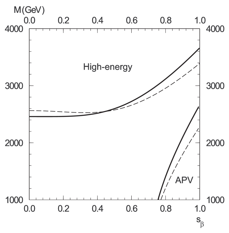
Figure 1: The 95% CL bounds on the compactification scale $M$ from the high-energy precision measurements ($\epsilon$ parameters) and from APV measurement. The solid and the dash lines correspond to $m_{H}=100~{}GeV$ and $m_{H}=300~{}GeV$ respectively.

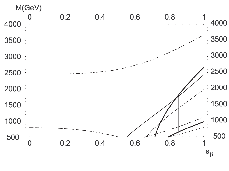
Figure 2: The 95% CL bounds on the compactification scale $M$ from the low-energy experiments: thick solid lines from $Q_{W}$ (the allowed region is the shadowed one); thin solid line from CHARM measurement of $R_{\nu}$; long dash lines from NuTeV; short dash line from CDHS measurement of $R_{\nu}$; dash-dot line from CCFR. The measurement of $R_{\bar{\nu}}$ gives no restrictions on the plane shown in the figure. For comparison we give also the bound from high-energy measurements, dash-dot-dot line. The SM values of the observables have been evaluated for a light Higgs mass.

References

• [1] T. Kaluza, Preuss. Akad. Wiss. (1921) 966.
• [2] O. Klein, Z. Phys. 37 (1926) 895.
• [3] For some recent literature, see for instance: I. Antoniadis, Phys. Lett. B246 (1990) 377; E. Witten, Nucl. Phys. B471 (1996) 135; J.D. Lykken, Phys. Rev. D54 (1996) 3693.
• [4] N. Arkani-Hamed, S. Dimopoulos and G. Dvali, Phys. Lett. B429 (1998) 263; I. Antoniadis, N. Arkani-Hamed, S. Dimopoulos and G. Dvali, Phys. Lett. B436 (1998) 257; N. Arkani-Hamed, S. Dimopoulos and G. Dvali, Phys. Rev. D59 (1999) 086004; K.R. Dienes, E. Dudas and T. Gherghetta Phys. Lett. B43(1998) 55.
• [5] A. Pomarol and M. Quiros, Phys. Lett. B438 255 (1998); A. Delgado, A. Pomarol and M. Quiros, hep-ph/9812489; M. Masip and A. Pomarol, hep-ph/9902467.
• [6] T.G. Rizzo and J.D. Wells, hep-ph/9906234; I. Antoniadis, K. Benakli, M. Quiros, Phys.Lett. B331 (1994) 313 ; ibidem hep-ph/9905311.
• [7] P. Nath and M. Yamaguchi, hep-ph/9902323; P. Nath and M. Yamaguchi, hep-ph/9903298, W.J. Marciano, hep-ph/9903451; A. Strumia, hep-ph/9906266.
• [8] G. Altarelli, R. Barbieri and S. Jadach, Nucl. Phys. B369 (1992) 3; G. Altarelli, R. Barbieri and F. Caravaglios Nucl. Phys. B405 (1993) 3; ibidem Phys. Lett. B349 (1995) 145.
• [9] M.E. Peskin and T. Takeuchi, Phys. Rev. Lett. 65 (1990) 964; ibidem Phys. Rev. D46 (1991) 381.
• [10] S.C. Bennett and C.E. Wieman, Phys. Rev. Lett. 82 (1999) 2484.
• [11] R. Casalbuoni, S. De Curtis, D. Dominici and R. Gatto, hep-ph/9905568.
• [12] C.P. Burgess, S. Godfrey, H. Konig, D. London, I. Maksymyk, Phys. Rev. D49 (1994) 6115; L. Anichini, R. Casalbuoni and S. De Curtis, Phys. Lett, B348 (1995) 521.
• [13] G. Altarelli, presented at the Blois Conference, June 1999.
• [14] G. Altarelli, R. Barbieri and F. Caravaglios, Int. J. Mod. Phys. A13 (1998) 1031.
• [15] M.C. Noecker, B.P. Masterson and C.E. Wieman, Phys. Rev. Lett. 61 (1988) 310.
• [16] S.A. Blundell, W.R. Johnson and J. Sapirstein, Phys. Rev. Lett. 65 (1990) 1411; V. Dzuba, V. Flambaum, P. Silvestrov and O. Sushkov, Phys. Lett. A141 (1989) 147.
• [17] W.J. Marciano and J.L. Rosner, Phys. Rev. Lett. 65 (1990) 2963.
• [18] See the second reference in [8].
• [19] For recent reviews of the subject see: D. Zeppenfeld and K. Cheung, hep-ph/9810277.
• [20] J. Erler and P. Langacker, hep-ph/9903476.
• [21] K.S. McFarland et al., hep-ex/9806013.
• [22] K.S. McFarland et al., Eur. Phys. J. C1 (1998) 509.
• [23] V. Allaby et al., Z. Physics C36 (1987) 611.
• [24] A. Blondel et al., Z. Physics C45 (1990) 361.
Refer to caption