Supernatural Supersymmetry:
Phenomenological Implications of
Anomaly-Mediated Supersymmetry Breaking

Abstract

We discuss the phenomenology of supersymmetric models in which supersymmetry breaking terms are induced by the super-Weyl anomaly. Such a scenario is envisioned to arise when supersymmetry breaking takes place in another world, i.e., on another brane. We review the anomaly-mediated framework and study in detail the minimal anomaly-mediated model parametrized by only $3+1$ parameters: $M_{\text{aux}}$, $m_{0}$, $\tan\beta$, and $\>\!\text{sign}\>\!(\mu)$. The renormalization group equations exhibit a novel “focus point” (as opposed to fixed point) behavior, which allows squark and slepton masses far above their usual naturalness bounds. We present the superparticle spectrum and highlight several implications for high energy colliders. Three lightest supersymmetric particle (LSP) candidates exist: the Wino, the stau, and the tau sneutrino. For the Wino LSP scenario, light Wino triplets with the smallest possible mass splittings are preferred; such Winos are within reach of Run II Tevatron searches. Finally, we study a variety of sensitive low energy probes, including $b\to s\gamma$, the anomalous magnetic moment of the muon, and the electric dipole moments of the electron and neutron.

I Introduction

Signals from supersymmetry (SUSY) are important targets for particle physics experiments. These signals range from the direct discovery of supersymmetric particles at high energy colliders to indirect signals at lower energy experiments through measurements of flavor-changing processes, magnetic and electric dipole moments, and so on. The set of possible signals and the promise of individual experiments for SUSY searches depend strongly on what model of SUSY breaking is assumed. It is therefore important to understand the characteristic features and predictions of well-motivated SUSY breaking scenarios.

Probably the most well-known scenario is that of SUSY breaking in the supergravity framework, i.e., “gravity-mediated” SUSY breaking. In this framework, SUSY breaking originates in a hidden sector and is transmitted to the observable sector though Planck scale-suppressed operators. In particular, soft masses for squarks, sleptons, and Higgs bosons are induced by direct Kähler interactions between hidden and observable sector fields. Unfortunately, these Kähler interactions are not, in general, flavor-diagonal. Squark and slepton mass matrices therefore typically have large flavor mixings, and these induce unacceptably large flavor-changing processes, such as $K^{0}$-$\bar{K}^{0}$ mixing and $\mu\to e\gamma$ [1]. These difficulties, together commonly referred to as the SUSY flavor problem, may be avoided if the Kähler potential is somehow constrained to be flavor-diagonal. Gauge-mediated SUSY breaking [2] is one proposal for solving this problem.

Recently the mechanism of “anomaly-mediated” SUSY breaking has been proposed as a possibility for generating (approximately) flavor-diagonal squark and slepton mass matrices [3]. In this scenario, SUSY is again broken in a hidden sector, but it is now transmitted to the observable sector dominantly via the super-Weyl anomaly [3, 4]. Gaugino and scalar masses are then related to the scale dependence of the gauge and matter kinetic functions. For first and second generation fields, whose Yukawa couplings are negligible, wavefunction renormalization is almost completely determined by gauge interactions. Their anomaly-mediated soft scalar masses are thus almost diagonal, and the SUSY flavor problem is solved. Note that this solution requires that the anomaly-mediated terms be the dominant contributions to the SUSY breaking parameters. This possibility may be realized, for example, if SUSY breaking takes place in a different world, i.e., on a brane different from the 3-brane of our world, and direct Kähler couplings are thereby suppressed [3].

As will be discussed below, the expressions for anomaly-mediated SUSY breaking terms are scale-invariant. Thus, they are completely determined by the known low energy gauge and Yukawa couplings and an overall mass scale $M_{\text{aux}}$. Anomaly-mediated SUSY breaking is therefore highly predictive, with fixed mass ratios motivating distinctive experimental signals, such as macroscopic tracks from highly degenerate Wino-like lightest supersymmetric particles (LSPs) [5, 6]. Unfortunately, one such prediction, assuming minimal particle content, is that sleptons are tachyons. Several possible solutions to this problem have already been proposed [3, 7, 8, 9]. We will adopt a phenomenological approach, first taken in Ref. [6], and assume that the anomaly-mediated scalar masses are supplemented by an additional universal contribution $m_{0}^{2}$. For large enough $m_{0}$, the slepton squared masses are positive. Along with the requirement of proper electroweak symmetry breaking, this defines the minimal anomaly-mediated model in terms of only 3+1 parameters: $M_{\text{aux}}$, $m_{0}$, $\tan\beta$, and $\>\!\text{sign}\>\!(\mu)$, where $\tan\beta$ is the ratio of Higgs vacuum expectation values (VEVs), and $\mu$ is the Higgsino mass parameter. The simplicity of this model allows one to thoroughly examine all of parameter space.

In this paper, we present a detailed study of the phenomenology of the minimal anomaly-mediated model. We begin in Sec. II with a brief discussion of the mechanism of anomaly-mediated SUSY breaking. In Sec. III we review the tachyonic slepton problem and the universal $m_{0}$ “solution,” and present in detail the minimal anomaly-mediated model described above. The universal scalar mass $m_{0}$ breaks the simple scale invariance of expressions for soft terms. However, this breaking is rather minimal, in a sense to be explained, and the minimal anomaly-mediated model inherits several simple properties from the pure anomaly-mediated case.

The naturalness of this model is examined in Sec. IV. We find that the minimal anomaly-mediated model exhibits a novel renormalization group (RG) “focus point” (as opposed to fixed point) behavior, which allows slepton and squark masses to be well above their usual naturalness bounds. The title “supernatural supersymmetry” derives from this feature and the envisioned other-worldly SUSY breaking.

We then turn in Sec. V to high-energy experimental implications. We explore the parameter space and find a variety of interesting features, including 3 possible LSP candidates: a degenerate triplet of Winos, the lighter stau $\tilde{\tau}_{1}$, and the tau sneutrino $\tilde{\nu}_{\tau}$. The Wino LSP scenario is realized in a large fraction of parameter space and has important new implications for both collider physics [5, 6] and cosmology [6, 10]. We find that naturalness and electroweak symmetry breaking favor light Winos with the smallest possible mass splittings, i.e., the ideal region of parameter space for Wino searches and within the discovery reach of Run II of the Tevatron.

While anomaly-mediated models have the virtue that they predict very little flavor-changing in the first and second generations, they are not therefore automatically safe from all low-energy probes. In Sec. VI we analyze several sensitive low-energy processes: $b\to s\gamma$, which probes flavor-changing in the third generation, and three important flavor-conserving observables, the anomalous magnetic dipole moment of the muon, and the electric dipole moments of the electron and neutron.

Our conclusions and final remarks are collected in Sec. VII. In the Appendix, we present expressions for anomaly-mediated SUSY breaking terms in a general supersymmetric theory and also the full flavor-dependent expressions for the specific case of the minimal anomaly-mediated model.

II Anomaly-Mediated Supersymmetry Breaking

In supergravity, SUSY breaking parameters always receive anomaly-mediated contributions. However, in the usual gravity-mediated SUSY breaking scenario, SUSY breaking masses also arise from direct interactions of observable sector fields with hidden sector SUSY breaking fields. Such contributions are usually comparable to the gravitino mass, and so anomaly-mediated contributions, which are loop-suppressed relative to the gravitino mass, are sub-leading. However, in a model with no direct coupling between observable and hidden sectors, the anomaly-mediated terms can be the dominant contributions. In this paper, we assume that this is the case, and that the anomaly-mediated terms are (one of) the leading contributions to the SUSY breaking parameters. This is realized, for example, in the “sequestered sector” model of Ref. [3], where the SUSY breaking sector and the observable sector are assumed to lie on different branes, thereby suppressing direct observable sector-hidden sector couplings.

In global SUSY, the (loop-corrected) effective Lagrangian may be written as

$${\cal L}_{\rm global}(\Box,\Lambda_{\rm cut}^{*},\Lambda_{\rm cut}) = \frac{1}{4}\int d^{2}\theta\left[\frac{1}{g^{2}}-\frac{b}{8\pi^{2}}\log(\Box^{1/2}/\Lambda_{\rm cut})\right]W^{\alpha}W_{\alpha}+{\rm h.c.}$$ (3)

$$+\int d^{4}\theta Z_{\phi}(\Box,\Lambda_{\rm cut}^{*}\Lambda_{\rm cut})\phi^{*}\phi$$

$$+\int d^{2}\theta Y\phi^{3}+{\rm h.c.}+\cdots\ ,$$

where $W^{\alpha}$ and $\phi$ are the gauge field strength and chiral superfields, respectively. Here $b$ is the $\beta$-function coefficient for the gauge coupling constant $g$, $Z_{\phi}$ is the wavefunction renormalization factor of $\phi$, $Y$ is the Yukawa coupling constant, and $\Lambda_{\rm cut}$ is the cut-off of the theory.

However, once we consider local SUSY, i.e., supergravity, this expression is modified. The most important modification for our argument results from the fact that, in global SUSY, $\Box$ is given by $g^{\mu\nu}\partial_{\mu}\partial_{\nu}$. In supergravity, $g^{\mu\nu}$ becomes a dynamical field and is part of the supergravity multiplet. $\Box$ must therefore be promoted to an object compatible with supergravity. The complete expression for $\Box$ is complicated. However, since we are interested only in the SUSY breaking terms, our task is simplified. Perhaps the easiest prescription for deriving the SUSY breaking terms is to introduce the compensator superfield $\Phi$, whose VEV is given by

$$\langle\Phi\rangle=1-M_{\text{aux}}\theta^{2}\ .$$ (4)

Here $M_{\rm aux}$ is proportional to the VEV of an auxiliary field in the supergravity multiplet and is of order the gravitino mass after SUSY breaking. With this compensator field, all of the terms relevant for calculating the anomaly-mediated SUSY breaking parameters are contained in the Lagrangian [3, 4] 

$${\cal L}_{\rm SUGRA}\simeq{\cal L}_{\rm global}(\Box,\Lambda_{\rm cut}^{*}\Phi^{*},\Lambda_{\rm cut}\Phi)\ .$$ (5)

Because $\Box$ appears in Eq. (3) only through terms $\Box^{1/2}/\Lambda_{\rm cut}$ and $\Box^{1/2}/\Lambda_{\rm cut}^{*}$, the replacement of $\Box$ by its supergravity generalization is effectively carried out by the replacement $\Lambda_{\rm cut}\to\Lambda_{\rm cut}\Phi$ [7].

Expanding the above Lagrangian with the VEV of $\Phi$ given in Eq. (4), and solving the equation of motion for the auxiliary component of $\phi$, the anomaly-mediated contributions to the gaugino mass $M_{\lambda}$, scalar squared mass $m^{2}$, and trilinear scalar coupling $A$ are

$$M_{\lambda}|_{\rm AM} = \frac{1}{16\pi^{2}}bg^{2}M_{\text{aux}}$$ (6)

$$m^{2}|_{\rm AM} = \frac{1}{2}\dot{\gamma}M_{\text{aux}}^{2}$$ (7)

$$A|_{\rm AM} = -\sum Y\gamma M_{\text{aux}}\ ,$$ (8)

where

$$\gamma\equiv-\frac{1}{2}\frac{dZ_{\phi}}{d\log\Box^{1/2}}\ ,\quad\dot{\gamma}\equiv\frac{d\gamma}{d\log\Box^{1/2}}\ .$$ (9)

Here $b$ and $\gamma$ are to be evaluated with the supersymmetric field content present at the appropriate scale. In the above formulae, indices have been suppressed. The full expressions for general chiral superfield content may be found in the Appendix.

One important feature of this result is that the formulae for the anomaly-mediated SUSY breaking parameters are RG-invariant [3, 4, 7, 11]. The anomaly-induced masses are given as functions of the gauge and Yukawa coupling constants, as shown in Eqs. (6) – (9), and the $\beta$-functions for the individual SUSY breaking parameters agree with the $\beta$-functions of the right-hand sides whose scale dependences are determined through the gauge and Yukawa coupling RG equations.

III The Minimal Anomaly-mediated Model

As described in the previous section, in pure anomaly-mediated SUSY breaking, soft terms are determined by RG-invariant expressions involving the gauge and Yukawa couplings. The soft terms are therefore completely fixed by the low energy values of these couplings and an overall scale $M_{\text{aux}}$. If a scalar has negligible Yukawa interactions, its squared mass is determined by gauge coupling contributions $-\sum_{i}b_{i}g_{i}^{4}$, where the sum is over all gauge groups under which the scalar is charged, and (positive) constants have been omitted (see Appendix). From this form, we see that sleptons, which interact only with non-asymptotically free groups ($b_{i}>0$), have negative squared masses. Tachyonic sleptons are the most glaring problem of the anomaly-mediated scenario.

Several mechanisms for solving the tachyonic slepton problem have been proposed. Additional positive contributions to slepton squared masses may arise from bulk contributions [3], gauge-mediated-like contributions [7], new Yukawa interactions [8], or non-decoupling higher order threshold effects [9]. Here, we adopt a simple phenomenological approach [6]: we assume an additional, universal, non-anomaly-mediated contribution $m_{0}^{2}$ to all scalars at the grand unified theory (GUT) scale $M_{\text{GUT}}$. The resulting boundary conditions,

$$M_{\lambda}(M_{\rm GUT}) = M_{\lambda}|_{\rm AM}(M_{\rm GUT})$$ (10)

$$m^{2}(M_{\rm GUT}) = m^{2}|_{\rm AM}(M_{\rm GUT})+m_{0}^{2}$$ (11)

$$A(M_{\rm GUT}) = A|_{\rm AM}(M_{\rm GUT})\ ,$$ (12)

define the minimal anomaly-mediated model. For large enough $m_{0}^{2}$, slepton squared masses are therefore positive, and the tachyonic slepton problem is averted. Such a universal term may be produced by bulk interactions [3], but is certainly not a feature common to all anomaly-mediated scenarios. The extent to which the following results depend on this assumption will be addressed in Sec. VII.

The addition of a non-anomaly-mediated term destroys the feature of RG invariance. However, the RG evolution of the resulting model nevertheless inherits some of the simplicity of the original pure anomaly-mediated relations. Schematically, scalar masses $m_{i}$ satisfy the one-loop RG equations

$$\frac{d}{dt}m^{2}_{i}\sim\frac{1}{16\pi^{2}}\left[-g^{2}M_{\lambda}^{2}+A^{2}+\sum_{j}Y^{2}m_{j}^{2}\right]\ ,$$ (13)

where $t\equiv\ln(\mu/M_{\text{GUT}})$, positive numerical coefficients have been omitted, and the sum is over all chiral fields $\phi_{j}$ interacting with $\phi_{i}$ through the Yukawa coupling $Y$. Letting $m_{i}^{2}\equiv m_{i}^{2}|_{\text{AM}}+\delta m_{i}^{2}$, where $m_{i}^{2}|_{\text{AM}}$ is the pure anomaly-mediated value, the RG invariance of the anomaly-mediated masses implies

$$\frac{d}{dt}\delta m^{2}_{i}\sim\frac{1}{16\pi^{2}}\sum_{j}Y^{2}\delta m_{j}^{2}\ .$$ (14)

Thus, at one-loop, the deviations from pure anomaly-mediated relations satisfy simple evolution equations that depend only on the deviations themselves. For scalars with negligible Yukawa couplings, such as the first and second generation squarks and sleptons, the deviation $\delta m^{2}_{i}$ is a constant of RG evolution. For them, $\delta m^{2}_{i}$ is simply an additive constant, and the weak scale result for $m^{2}_{i}$ is independent of the scale at which $\delta m_{i}^{2}$ is generated. For fields interacting through large Yukawa couplings such as the top Yukawa coupling, the deviations $\delta m_{i}^{2}$ evolve; however, this evolution is simply analyzed. We will see an important consequence of this evolution for naturalness in Sec. IV.

We will assume that the boundary conditions of Eq. (11) are given at $M_{\rm GUT}=2\times 10^{16}~{}{\rm GeV}$. The SUSY breaking parameters are then evolved with one-loop RG equations to the superparticle mass scale $m_{\rm SUSY}$, which we have approximated to be the squark mass scale. For the gaugino mass parameters, we also include the largest next-to-leading order corrections from $\alpha_{s}$ and $\alpha_{t}\equiv y_{t}^{2}/4\pi$ given in Ref. [6].

All parameters of the theory are then specified, except for $\mu$, the Higgsino mass parameter, and $B_{\mu}$, the soft bilinear Higgs coupling. We do not specify the mechanism for generating these parameters, but assume that they are constrained so that electroweak symmetry is properly broken. Given the other soft parameters at $m_{\rm SUSY}$, the Higgs potential is determined by $\mu$ and $B_{\mu}$, or alternatively, by the Fermi constant $G_{\rm F}=[2\sqrt{2}(\langle H_{u}^{0}\rangle^{2}+\langle H_{d}^{0}\rangle^{2})]^{-1}\simeq 1.17\times 10^{-5}~{}{\rm GeV}^{-2}$ (or, equivalently, the $Z$ mass) and $\tan\beta=\langle H_{u}^{0}\rangle/\langle H_{d}^{0}\rangle$. It is more convenient to use the latter two as inputs; $\mu$ and $B_{\mu}$ are then fixed so that the Higgs potential has a proper minimum with correct $G_{\rm F}$ and $\tan\beta$. We minimize the Higgs potential at one-loop, including radiative corrections from third generation quarks and squarks [12], but neglecting radiative corrections from other particles.

In fact, the constraint of proper electroweak symmetry breaking does not determine the sign of the $\mu$ parameter. The entire parameter space of the minimal anomaly-mediated model is therefore specified by 3+1 parameters:

$$M_{\text{aux}},m_{0},\tan\beta,\ \text{and}\ \>\!\text{sign}\>\!(\mu)\ .$$ (15)

IV Naturalness

Supersymmetric theories are considered natural from the point of view of the gauge hierarchy problem if the electroweak scale is not unusually sensitive to small variations in the underlying parameters. There are a variety of prescriptions for quantifying naturalness with varying degrees of sophistication [13]. For the present purposes, we simply consider a set of parameters to be natural if no large cancellations occur in the determination of the electroweak scale. At tree-level, the relevant condition is

$$\frac{1}{2}m_{Z}^{2}=\frac{m_{H_{d}}^{2}-m_{H_{u}}^{2}\tan^{2}\beta}{\tan^{2}\beta-1}-\mu^{2}\ ,$$ (16)

where $m_{H_{u}}^{2}$ and $m_{H_{d}}^{2}$ are the soft SUSY breaking masses for up- and down-type scalar Higgses. Naturalness then requires that $|\mu|$ as determined from electroweak symmetry breaking not be too far above the electroweak scale. A typical requirement is $|\mu|\lesssim 1\text{ TeV}$.

In Fig. 1 we present values of $\mu$ in the $(m_{0},M_{\text{aux}})$ plane for three representative values of $\tan\beta$: 3 (low), 10 (moderate), and 30 (high). We have chosen $\mu<0$ to avoid constraints from $b\to s\gamma$ at large $\tan\beta$ (see Sec. VI A), but similar $|\mu|$ are found for $\mu>0$. The parameter $M_{\text{aux}}$ is not phenomenologically transparent, and so on the right-hand axis, we also give approximate values of the Wino mass $M_{2}$, using $M_{2}=\frac{g_{2}^{2}}{16\pi^{2}}M_{\text{aux}}\simeq 2.9\times 10^{-3}M_{\text{aux}}$.

The value of $|\mu|$ rises with increasing $M_{\text{aux}}$, as expected. Irrespective of $m_{0}$ and $\tan\beta$, $|\mu|\lesssim 1\text{ TeV}$ implies $M_{2}\lesssim 200\text{ GeV}$. Such a restriction is encouraging for searches for degenerate Winos at upcoming runs of the Tevatron, as will be discussed more fully in Sec. V A.

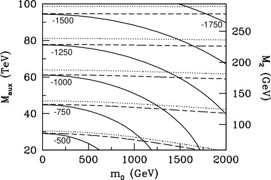
FIG. 1.: Contours of constant $\mu<0$ in GeV for $\tan\beta=3$ (solid), 10 (dashed), and 30 (dotted). The value of $|\mu|$ is similar for $\mu>0$.

The special case of $m_{0}=0$ corresponds to pure anomaly-mediated SUSY breaking. In this case, the expressions for soft SUSY breaking terms are RG-invariant and the soft masses may be evaluated at any scale, including a low (TeV) scale. Based on this observation, it has been argued that, since the stop masses do not enter the determination of $m_{H_{u,d}}^{2}$ with large logarithms through RG evolution, stop masses of $2\text{ TeV}$ or even higher are consistent with naturalness [3]. This is contradicted by Fig. 1: for $m_{0}=0$, as will be seen in Sec. V C, stop masses of $2\text{ TeV}$ require very large $M_{\text{aux}}$ corresponding to values of $|\mu|$ above 2 TeV. Stop masses of 2 TeV are therefore as unnatural in pure anomaly-mediated SUSY breaking as they are in more conventional gravity-mediated scenarios, such as minimal supergravity. This applies to all cases where the pure anomaly-mediated relations are approximately valid for squark and Higgs soft masses, and includes models in which a mechanism for avoiding tachyonic sleptons is invoked which does not disturb the squark and Higgs masses.

For the minimal anomaly-mediated model with $m_{0}>0$, however, the squark and Higgs masses are explicitly modified, and the argument above does not apply. It is exactly in this case, where the soft SUSY masses are not RG-invariant, that there is the possibility that heavy squarks can be consistent with naturalness, and we will see that, in fact, this is realized by a novel mechanism for large $m_{0}$.

In Fig. 1, for $\tan\beta=3$, an upper bound on $|\mu|$ implies an upper bound on $m_{0}$. However, for moderate and large $\tan\beta$, the contours of constant $|\mu|$ are extremely insensitive to $m_{0}$, and so large squark and slepton masses are consistent with naturalness in the large $m_{0}$ regime. This behavior may be understood first by noting that, for moderate and large $\tan\beta$, Eq. (16) implies that $\mu$ depends sensitively on $m_{H_{u}}^{2}$ only. The RG evolution of $m_{H_{u}}^{2}$ is most easily understood by letting $m_{H_{u}}^{2}\equiv m_{H_{u}}^{2}|_{\text{AM}}+\delta m_{H_{u}}^{2}$, where $m_{H_{u}}^{2}|_{\text{AM}}$ is the pure anomaly-mediated value, and similarly for all other scalar masses. The deviations $\delta m_{i}^{2}$ satisfy simple RG equations, as discussed in Sec. III. For $\tan\beta$ not extremely large, the only large Yukawa is the top Yukawa $Y_{t}$, and $m_{H_{u}}^{2}$ is determined by the system of RG equations

$$\frac{d}{dt}\left(\begin{array}[]{c}\delta m_{H_{u}}^{2}\\ \delta m_{U_{3}}^{2}\\ \delta m_{Q_{3}}^{2}\end{array}\right)=\frac{Y_{t}^{2}}{8\pi^{2}}\left(\begin{array}[]{ccc}3&3&3\\ 2&2&2\\ 1&1&1\end{array}\right)\left(\begin{array}[]{c}\delta m_{H_{u}}^{2}\\ \delta m_{U_{3}}^{2}\\ \delta m_{Q_{3}}^{2}\end{array}\right)\ ,$$ (17)

where $Q_{3}$ and $U_{3}$ denote the third generation squark SU(2) doublet and up-type singlet representations, respectively.

Such systems of RG equations are easily solved by decomposing arbitrary initial conditions into components parallel to the eigenvectors of the evolution matrix, which then evolve independently [14]. In the present case, the solution with initial condition $m_{0}^{2}(1,1,1)^{T}$ is

$$\left(\begin{array}[]{c}\delta m_{H_{u}}^{2}\\ \delta m_{U_{3}}^{2}\\ \delta m_{Q_{3}}^{2}\end{array}\right)=\frac{m_{0}^{2}}{2}\left(\begin{array}[]{c}3\\ 2\\ 1\end{array}\right){\rm exp}\left[6\int_{0}^{t}\frac{Y_{t}^{2}}{8\pi^{2}}dt^{\prime}\right]-\frac{m_{0}^{2}}{2}\left(\begin{array}[]{c}1\\ 0\\ -1\end{array}\right)\ .$$ (18)

For $t$ and $Y_{t}$ such that ${\rm exp}\left[6\int_{0}^{t}\frac{Y_{t}^{2}}{8\pi^{2}}dt^{\prime}\right]=1/3$, $\delta m_{H_{u}}^{2}=0$, i.e., $m_{H_{u}}^{2}$ assumes its pure anomaly-mediated value for any $m_{0}$.

The RG evolution of $m_{H_{u}}^{2}$ is shown for several values of $m_{0}$ in Fig. 2. As expected, the RG curves intersect at a single point where $m_{H_{u}}^{2}$ is independent of $m_{0}$; we will call this a “focus point.” Remarkably, however, the focus point occurs near the weak scale for $Y_{t}$ corresponding to the physical top mass of $m_{\text{top}}\approx 174\text{ GeV}$. Thus the weak scale value of $m_{H_{u}}^{2}$ is nearly its pure anomaly-mediated value for all values of $m_{0}$. Note that this behavior applies only to $m_{H_{u}}^{2}$; no other scalar mass has a focus point behavior.

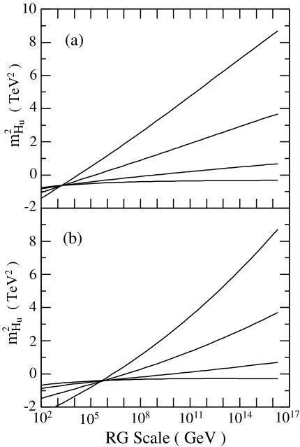
FIG. 2.: The RG evolution of $m_{H_{u}}^{2}$ for fixed $M_{\text{aux}}=50\text{ TeV}$, $\tan\beta=10$, and top quark mass (a) 174 GeV (b) 184 GeV. The GUT scale boundary conditions are for $m_{0}=0,1,2,3\text{ TeV}$, from the bottom. The RG behavior of $m_{H_{u}}^{2}$ exhibits a focus point (not a fixed point) near the weak scale, where $m_{H_{u}}^{2}$ takes its pure anomaly-mediated value, irrespective of $m_{0}$.

The focus point is not a fixed point; for example, below the focus point, the RG curves diverge again. The position of the focus point depends on $Y_{t}$, and we must check the sensitivity to variations in $Y_{t}$. In Fig. 2 we show also the behavior for $Y_{t}$ corresponding to $m_{\text{top}}=184$ GeV. The exact weak scale value of $m_{H_{u}}^{2}$ depends on $Y_{t}$ and, when the focus point is not exactly at the weak scale, also on $m_{0}$. However, for top quark masses near the physical one, the focus point remains within a couple of decades of the weak scale, and the sensitivity to variations in $m_{0}$ is always suppressed. This is demonstrated in Fig. 3, where values of $\mu$ are given in the $(m_{0},m_{\text{top}})$ plane. Even for $m_{0}^{2}=25\text{ TeV}^{2}$ and $m_{\text{top}}=174\pm 5\text{ GeV}$, we find that $\mu^{2}$ lies naturally below 2 $\text{ TeV}^{2}$.

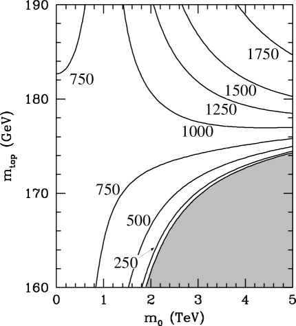
FIG. 3.: Contours of $|\mu|$ in GeV for $\mu<0$, $M_{\text{aux}}=50\text{ TeV}$, and $\tan\beta=10$. In the shaded region, electroweak symmetry cannot be broken radiatively.

An interesting question is whether $m_{0}$ can be bigger than the weak scale by a loop factor without compromising naturalness. If this were the case, there would be no need to appeal to a sequestered sector to eliminate tree-level scalar masses. However, $m_{0}$ cannot be arbitrarily large. In Fig. 3, we see that the requirement of proper electroweak symmetry breaking implies $m_{0}\lesssim 5\text{ TeV}$. In any case, a similar bound would follow from requiring that one-loop finite corrections to the Higgs squared mass parameter, which are proportional to $m_{\tilde{f}}^{2}$, not introduce large fine-tunings. The maximum allowed $m_{0}^{2}$ is thus roughly an order of magnitude below $M_{\text{aux}}^{2}$. Thus, while it is possible to eliminate the sequestered seor mechanism for direct Kähler interaction suppression, it is still required that the tree-level scalar squared mass $m_{0}^{2}$ be suppressed by an order of magnitude relative to its “natural” value $\sim M_{\text{aux}}^{2}$.

Nevertheless, given that we have no understanding of the source of $m_{0}$, it is at least somewhat reassuring that it may be far above the weak scale without incurring a fine-tuning penalty. A direct consequence of this is that the minimal anomaly-mediated model is a model that naturally accommodates multi-TeV sleptons and squarks. As we will see below, this has important phenomenological consequences both for high energy colliders and low energy probes.

V Superpartner Spectra and Implications for High Energy Colliders

Having defined the minimal anomaly-mediated model in Sec. III and explored the natural range of its fundamental parameters in Sec. IV, we now consider the resulting masses and mixings of the superpartners. The lightest supersymmetric particles are either a degenerate triplet of charginos and neutralinos, the lighter stau $\tilde{\tau}_{1}$, or the tau sneutrino $\tilde{\nu}_{\tau}$. We begin by considering these, and conclude with a discussion of the squark spectrum. We do not discuss the gluino and heavy Higgses in detail. However, their masses are given in Eq. (19) and Figs. 13 and 14, respectively.

A Charginos and Neutralinos

Charginos and neutralinos are mixtures of gauginos and Higgsinos. Their composition is determined by $M_{2}$, $M_{1}$, $\mu$, and $\tan\beta$ at tree-level. Inserting the values of the gauge coupling constants at $m_{Z}$ in Eq. (6), and including the largest next-to-leading corrections as described in Sec. III, we find

$$M_{1}:M_{2}:M_{3}\approx 2.8:1:-8.3\ .$$ (19)

Typical values of $(\mu,M_{2})$ allowed by radiative electroweak symmetry breaking in the minimal anomaly-mediated model are given in Fig. 4. Combined with the anomaly-mediated relation $M_{1}\simeq 2.8M_{2}$, Fig. 4 implies $M_{2}<M_{1}<|\mu|$ with substantial hierarchies in these parameters throughout parameter space. The chargino and neutralino mass eigenstates are therefore well-approximated by pure gaugino and pure Higgsino states with masses

$$M_{2}: \tilde{\chi}^{0}_{1}\simeq\tilde{W}^{0}\ ,\ \tilde{\chi}^{\pm}_{1}\simeq\tilde{W}^{\pm}$$ (20)

$$M_{1}: \tilde{\chi}^{0}_{2}\simeq\tilde{B}$$ (21)

$$|\mu|: \tilde{\chi}^{0}_{3,4}\simeq\tilde{H}_{u}^{0}\pm\tilde{H}_{d}^{0}\ ,\ \tilde{\chi}^{\pm}_{2}\simeq\tilde{H}^{\pm}\ ,$$ (22)

and the lightest of these is always a highly degenerate triplet of Winos.

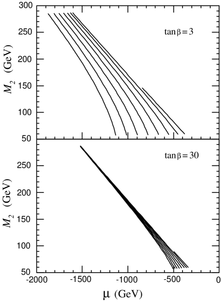
FIG. 4.: Parameters allowed by current constraints on particle masses and radiative symmetry breaking in the $(\mu,M_{2})$ plane for $\mu<0$ and $\tan\beta=3$ and 30. The contours are for constant $m_{0}=250$, 500, $\cdots$, 2000 GeV from the right. Similar results hold for $\mu>0$.

In much of parameter space, as we will see in Sec. V B, these Winos are the LSPs. The possibility of searching for supersymmetry in the Wino LSP scenario has been the subject of much recent attention [5, 6, 15, 16, 17]. The detection of Wino LSPs poses novel experimental challenges. Neutral Winos pass through collider detectors without interacting. Charged Winos are detectable in principle, but are typically highly degenerate with neutral Winos, with $\Delta m=m_{\tilde{\chi}^{\pm}_{1}}-m_{\tilde{\chi}^{0}_{1}}\approx 150-300\text{ MeV}$ and corresponding decay lengths $c\tau=0.5-10$ cm [5, 6, 15, 16, 17, 18]. They therefore decay to invisible neutral Winos and extremely soft pions before reaching the muon chambers, thereby escaping both conventional searches based on energetic decay products and searches for long-lived charged particles that produce hits in the muon chamber.

Fig. 4, however, has two important and encouraging implications for Wino LSP searches. First, as noted in Sec. IV, naturalness bounds on $|\mu|$ imply stringent bounds on $M_{2}$. From Fig. 4, for example, we find that $|\mu|\lesssim 1\text{ TeV}$ implies $M_{2}\lesssim 200\text{ GeV}$. Continuing searches at LEP [19], although limited kinematically to the region $M_{2}\lesssim 100\text{ GeV}$, will be able to probe a significant fraction of this parameter region. In addition, such limits on the Wino mass imply large cross sections at the Tevatron. For $M_{2}=200\text{ GeV}$ and $\sqrt{s}=2\text{ TeV}$, the Wino pair production rate is $\sigma(p\bar{p}\to\tilde{W}^{\pm}\tilde{W}^{0},\tilde{W}^{\pm}\tilde{W}^{\mp})\approx 100$ fb, and if a jet with $p_{T}>30\text{ GeV}$ and $|\eta|<2$ is required for triggering, the associated production rate is $\sigma(p\bar{p}\to\tilde{W}^{\pm}\tilde{W}^{0}+\text{ jet},\tilde{W}^{\pm}\tilde{W}^{\mp}+\text{ jet})\approx 10$ fb [5]. Such cross sections imply hundreds of Wino pairs produced at the upcoming Run II, and tens of Wino pairs produced in association with jets.

Second, the region of $(\mu,M_{2})$ space favored in Fig. 4 is the far gaugino region, where $\Delta m$ is minimized. For the parameters of Fig. 4, $\Delta m<180\text{ MeV}$, corresponding to decay lengths of $c\tau>3.5$ cm. (See Ref. [5].) Thus, a significant fraction of Winos will pass through several vertex detector layers. When produced in association with a jet for triggering, such Winos will be discovered off-line as high $dE/dx$ tracks with no associated calorimeter or muon chamber activity. Such a signal should be spectacular and background-free. This possibility is discussed in detail in Ref. [5], where an integrated luminosity of 2 $\text{ fb}^{-1}$ is shown to probe the entire region discussed here with $|\mu|<1\text{ TeV}$. It is exciting that Run II of the Tevatron will either discover Wino LSPs or exclude most of the natural region of parameter space in this model.

B Sleptons

Slepton masses and mixings are given by the mass matrix

$$\mbox{\boldmath$M_{\tilde{l}}^{2}$}=\left(\begin{array}[]{cc}m_{\tilde{L}}^{2}+m_{l}^{2}-m_{Z}^{2}(\frac{1}{2}-\sin^{2}\theta_{W})\cos 2\beta&m_{l}(A_{l}-\mu\tan\beta)\\ m_{l}(A_{l}-\mu\tan\beta)&m_{\tilde{E}}^{2}+m_{l}^{2}-m_{Z}^{2}\sin^{2}\theta_{W}\cos 2\beta\end{array}\right)$$ (23)

in the basis $(\tilde{l}_{L},\tilde{l}_{R})$, and sneutrino masses are given by

$$m_{\tilde{\nu}}^{2}=m_{\tilde{L}}^{2}+\frac{1}{2}m_{Z}^{2}\cos 2\beta\ ,$$ (24)

where $m_{\tilde{L}}^{2}$ and $m_{\tilde{E}}^{2}$ are the soft SUSY breaking masses.

In anomaly-mediated models, as discussed in Ref. [6], if both $m_{\tilde{L}}^{2}$ and $m_{\tilde{E}}^{2}$ receive the same $m_{0}^{2}$ contribution, the diagonal entries of the slepton mass matrix are accidentally highly degenerate. The anomaly-mediated boundary conditions imply (see the Appendix)

$$\mbox{\boldmath$M_{\tilde{l}}^{2}$}_{LL}-\mbox{\boldmath$M_{\tilde{l}}^{2}$}_{RR}=\frac{3}{2}\left(\frac{g_{2}^{2}M_{\text{aux}}}{16\pi^{2}}\right)^{2}\left[11\tan^{4}\theta_{W}-1\right]+m_{Z}^{2}\left[2\sin^{2}\theta_{W}-\frac{1}{2}\right]\cos 2\beta\ .$$ (25)

For $\sin^{2}\theta_{W}=0.2312$, $\tan^{4}\theta_{W}=0.0904$, and both bracketed expressions are extremely small. This accidental degeneracy implies that same-flavor sleptons may be highly degenerate. The physical mass splitting for staus is given in Fig. 5. For low $\tan\beta$ (and, by implication, for all $\tan\beta$ for selectrons and smuons), degeneracies of order 10 GeV or less are found throughout the parameter region. For large $\tan\beta$, however, large Yukawa effects dilute the degeneracy significantly.

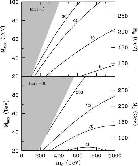
FIG. 5.: Contours of constant $m_{\tilde{\tau}_{2}}-m_{\tilde{\tau}_{1}}$ in GeV for $\mu<0$ and $\tan\beta=3$ and 30. The shaded region is excluded by $m_{\tilde{\tau}_{1}}>70\text{ GeV}$.

Equation (25) also implies that even small off-diagonal entries may lead to large mixing. The left-right mixing for staus is given in Fig. 6. Throughout parameter space, and even for low $\tan\beta$, the stau mixing is nearly maximal. In fact, even smuon mixing may be significant — for large $\tan\beta$ and low $M_{\text{aux}}$, it too is almost maximal. Nearly degenerate and highly-mixed same flavor sleptons are a distinctive feature of the minimal anomaly-mediated model and distinguish it from other gravity- and gauge-mediated models, where, typically, $m_{\tilde{l}_{L}}>m_{\tilde{l}_{R}}$. These features may be precisely tested by measurements of slepton masses [20] and mixings [21] at future colliders.

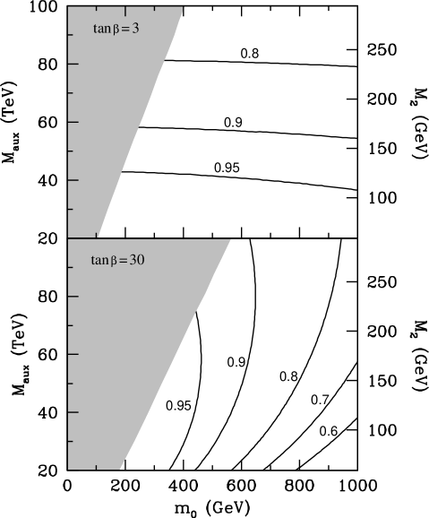
FIG. 6.: Contours of constant $|\sin 2\theta^{\tilde{\tau}}_{LR}|$ for $\mu<0$ and $\tan\beta=3$ and 30. The shaded region is excluded by $m_{\tilde{\tau}_{1}}>70\text{ GeV}$.

The lighter stau $\tilde{\tau}_{1}$ is always the lightest charged slepton, and it therefore plays an important phenomenological role. The $\tilde{\tau}_{1}$ mass is displayed in Fig. 7.

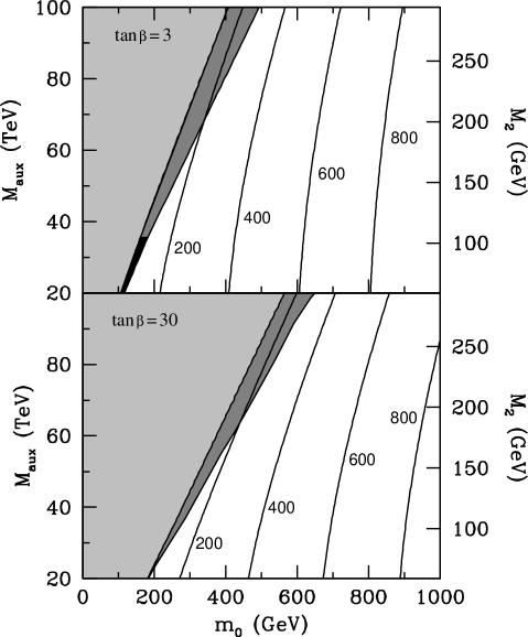
FIG. 7.: Contours of constant $m_{{\tilde{\tau}}_{1}}$ in GeV for $\mu<0$ and $\tan\beta=3$ and 30. The light shaded region is excluded by $m_{\tilde{\tau}_{1}}>70\text{ GeV}$. In the dark shaded region, the LSP is $\tilde{\tau}_{1}$, in the blackened region, the LSP is $\tilde{\nu}_{\tau}$, and in the unshaded region, the LSPs are a highly degenerate triplet of Winos.

For low $m_{0}$, $\tilde{\tau}_{1}$ is either tachyonic or excluded by experimental bounds. The current bounds are fairly complicated in this model, since the mass ordering and mass splittings between $\tilde{\tau}_{1}$, the Winos, and the sneutrinos vary throughout the parameter space. For staus decaying to neutralinos with a mass splitting greater than 15 GeV, combined LEP analyses of the $\sqrt{s}=189\text{ GeV}$ data yield the bound $m_{\tilde{\tau}}>71\text{ GeV}$ [22], but this drops to near the LEP I limit of 45 GeV as the mass splitting goes to zero. However, for stable staus, combined LEP analyses of data up to $\sqrt{s}=183\text{ GeV}$ imply $m_{\tilde{\tau}}>87\text{ GeV}$ [22]. The light shaded region of Fig. 7 is excluded by $m_{\tilde{\tau}}>70\text{ GeV}$ and represents a rough summary of these bounds. In the remaining region, the bounds $m_{\tilde{\nu}}>43\text{ GeV}$ [23], $m_{\tilde{e}}>89\text{ GeV}$ [22], and $m_{\tilde{\mu}}>84\text{ GeV}$ [22] are always satisfied. In the following, we will include the excluded shaded region in plots of observables that involve sleptons. For quantities such as squark masses or rates for $b\to s\gamma$, we omit this, as such quantities are well-defined even for small $m_{0}$, and in fact, the $m_{0}=0$ axis gives their values in anomaly-mediated models where the slepton mass problem is fixed without changing the squark and Higgs masses.

For large $m_{0}$, $m_{\tilde{\tau}_{1}}\approx m_{0}$, and the Wino is the LSP. This is the case in the unshaded region of Fig. 7. The experimental implications of the Wino LSP scenario have been discussed above in Sec. V A.

Finally, there exists an intermediate $m_{0}$ region, in which the LSP is either the $\tilde{\tau}_{1}$ or the $\tilde{\nu}_{\tau}$. In the $\tilde{\tau}_{1}$ LSP scenario (the dark shaded region of Fig. 7), the stau may be found at both LEP and the Tevatron through its spectacular anomalous $dE/dx$ and time-of-flight signatures [22, 24, 25]. At the Tevatron, for example, for $m_{\tilde{\tau}_{1}}\lesssim 150\text{ GeV}$, $\sigma(p\bar{p}\to\tilde{\tau}_{1}\tilde{\tau}_{1}^{*})\gtrsim 1$ fb, and so a significant fraction of the stau LSP parameter space may be explored.

In the case of the sneutrino LSP (the blackened region of Fig. 7), there are many possible experimental signatures. While this region appears only for a limited range of SUSY parameters, superparticles tend to be relatively light in this region, with $m_{\tilde{\tau}_{1}}\lesssim 100\text{ GeV}$ and $M_{2}\lesssim 110\text{ GeV}$, and so it is amenable to study at LEP. In this region, the slepton mass ordering is always

$$\tilde{\nu}_{\tau},\tilde{\nu}_{\mu},\tilde{\nu}_{e}<\tilde{\tau}_{1}<\tilde{e}_{R},\tilde{\mu}_{1}<\tilde{e}_{L},\tilde{\mu}_{2}<\tilde{\tau}_{2}\ ,$$ (26)

and the Wino triplet may appear anywhere between the sneutrinos and $\tilde{\tau}_{2}$. Typically, though not always, the only kinematically accessible superparticles at LEP are the sneutrinos, $\tilde{\tau}_{1}$ and the Winos. The two possible mass orderings and dominant decay modes in each scenario are then

$$\tilde{\tau}_{1}>\tilde{W}^{\pm,0}>\tilde{\nu}:\ \tilde{\tau}_{1}\to\tau\tilde{W}^{0},\nu_{\tau}\tilde{W}^{\pm}$$ (28)

$$\tilde{W}^{0}\to\nu_{l}\tilde{\nu}_{l}\ ,\ \tilde{W}^{\pm}\to l\tilde{\nu}_{l}$$

$$\tilde{W}^{\pm,0}>\tilde{\tau}_{1}>\tilde{\nu}:\ \tilde{W}^{0}\to\nu\tilde{\nu},\tau\tilde{\tau}_{1}\ ,\ \tilde{W}^{\pm}\to l\tilde{\nu}_{l},\nu_{\tau}\tilde{\tau}_{1}$$ (30)

$$\tilde{\tau}_{1}\to\pi^{\pm}\tilde{\nu}_{\tau}\ .$$

C Squarks

In anomaly-mediated SUSY breaking, squarks are universally very heavy, as their masses receive contributions from the strong coupling. The gauge coupling contribution to scalar squared masses is of the form $-b_{i}g_{i}^{4}$, where $b_{i}$ is the one-loop $\beta$-function coefficient (see Appendix), and so the strong coupling contribution completely overwhelms those of the SU(2) and U(1) couplings. Squark masses for the first two generations are therefore both flavor- and chirality-blind; we find that the $\tilde{u}_{L}$, $\tilde{u}_{R}$, $\tilde{d}_{L}$, and $\tilde{d}_{R}$, and their second generation counterparts are all degenerate to within $\sim 10$ GeV throughout parameter space.

The first and second generation squark masses are given in Fig. 8. The squarks are hierarchically heavier than Winos and sleptons for low $m_{0}$, and their mass increases as $m_{0}$ increases. For $m_{0}\gtrsim 2\text{ TeV}$, the squark mass is above 2 TeV. Thus, the focus point naturalness behavior discussed in Sec. IV, which allows such large $m_{0}$, has important phenomenological consequences. Direct detection of 2 TeV squarks is likely to be impossible at the LHC or NLC, and must wait for even higher energy hadron or muon colliders. Note, however, that some superparticles, notably the gauginos, cannot evade detection at the LHC and NLC.

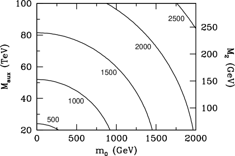
FIG. 8.: Contours of constant $m_{\tilde{u}_{L}}$ in GeV for $\mu<0$. The masses of all first and second generation squarks are degenerate to within $\sim 10$ GeV throughout the parameter space and are insensitive to $\tan\beta$.

Unlike the squarks of the first two generations, the masses of third generation squarks $\tilde{t}_{L}$, $\tilde{t}_{R}$, $\tilde{b}_{L}$, and (for large $\tan\beta$) $\tilde{b}_{R}$ receive significant contributions from large Yukawa couplings. These are shown in Figs. 9 and 10 for small and large values of $\tan\beta$. Yukawa couplings always reduce the masses and their effect may be large. For example, $m_{\tilde{t}_{1}}$ may be reduced by as much as 40% relative to the first and second generation squark masses. At the LHC, therefore, stops and sbottoms may be produced in much larger numbers than the other squarks, adding to the importance of $b$-tagging.

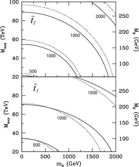
FIG. 9.: Contours of constant $m_{\tilde{t}_{2}}$ and $m_{\tilde{t}_{1}}$ in GeV for $\mu<0$ and $\tan\beta=3$ (solid) and 30 (dotted).

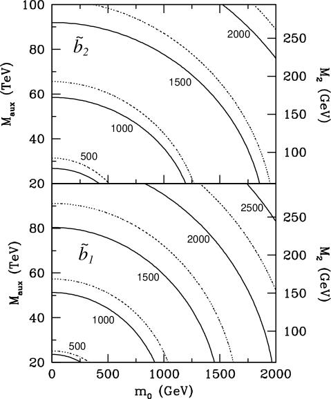
FIG. 10.: Contours of constant $m_{\tilde{b}_{2}}$ and $m_{\tilde{b}_{1}}$ in GeV for $\mu<0$ and $\tan\beta=3$ (solid) and 30 (dotted).

As in the case of sleptons, third generation squarks may have large left-right mixing. For $\tan\beta=30$, left-right mixing in both the stops and sbottoms is large, and is nearly maximal for low $m_{0}$. For $\tan\beta=3$, sbottom mixing is negligible, but stop mixing may still be as large as $\sin 2\theta^{\tilde{t}}_{LR}\approx 0.2$.

VI Low Energy Probes

Anomaly-mediated supersymmetry breaking naturally suppresses flavor-violation in the first and second generations, but not all low energy constraints are therefore trivially satisfied. In particular, since anomaly-mediated soft terms depend on Yukawa couplings, non-trivial flavor mixing involving third generation squarks can be expected. We first study the flavor-changing process $b\to s\gamma$, which is well-known for being sensitive to third generation flavor violation. We then consider magnetic and electric dipole moments, observables that are flavor-conserving, but are nevertheless highly sensitive to SUSY effects.

A $b\to s\gamma$

In the standard model, the flavor-changing transition $b\to s\gamma$ is mediated by a $W$ boson at one-loop. In supersymmetric theories, $b\to s\gamma$ receives additional one-loop contributions from charged Higgs-, chargino-, gluino-, and neutralino-mediated processes. The charged Higgs contribution depends only on the charged Higgs mass and $\tan\beta$, interferes constructively with the standard model amplitude, and is known to be large even for charged Higgs masses beyond current direct experimental bounds. The supersymmetric contributions may also be large for some ranges of SUSY parameters. Thus, $b\to s\gamma$ provides an important probe of all supersymmetric models, including those that are typically safe from other flavor-violating constraints.

In the well-studied cases of minimal supergravity and gauge-mediated SUSY breaking [27], the chargino- and, to a lesser extent, gluino-mediated contributions may be significant for large $\tan\beta$. Neutralino contributions are always negligible. For $\mu<0$ (in our conventions), these contributions are constructive and so, for large $\tan\beta$, positive $\mu$ is favored.

In the present case of anomaly-mediated SUSY breaking, several new features arise. First, in contrast to the case of minimal supergravity and gauge-mediation where squark mixing arises only through RG evolution, flavor violation in the squark sector is present even in the boundary conditions (and receives additional contributions from RG evolution). More importantly, the signs of the parameter $A_{t}$ and the gluino mass $M_{3}$ are opposite to those of minimal supergravity and gauge-mediation. The leading contributions for large $\tan\beta$ in the mass insertion approximation from charginos and gluinos are given in Fig. 11. For large $\tan\beta$, the amplitudes ${\cal A}_{\tilde{\chi}^{\pm}}\propto\>\!\text{sign}\>\!(\mu A_{t})$ and ${\cal A}_{\tilde{g}}\propto\>\!\text{sign}\>\!(\mu M_{3})$ are both opposite in sign relative to their values in minimal supergravity and gauge-mediation.

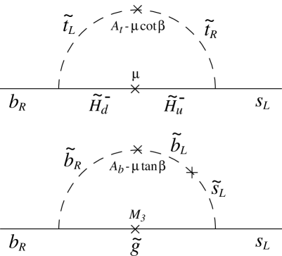
FIG. 11.: The leading contributions to $b\to s\gamma$ from chargino- and gluino-mediated processes in the mass insertion approximation for large $\tan\beta$. The photon, which may couple to any charged internal propagator, is omitted.

$B(B\to X_{s}\gamma)$ may be calculated by first matching the full supersymmetric theory on to the effective Hamiltonian

$${\cal H}_{\text{eff}}=-\frac{4G_{F}}{\sqrt{2}}V^{*}_{ts}V_{tb}\sum_{i=1}^{8}C_{i}{\cal O}_{i}$$ (31)

at the electroweak scale $m_{W}$. In the basis where the current and mass eigenstates are identified for $d_{L}$, $d_{R}$, and $u_{R}$, supersymmetry contributes dominantly to the Wilson coefficients $C_{7}$ and $C_{8}$ of the magnetic and chromomagnetic dipole operators

$${\cal O}_{7} = \frac{e}{16\pi^{2}}m_{b}(\bar{s}_{L}\sigma^{\mu\nu}b_{R})F_{\mu\nu}$$ (32)

$${\cal O}_{8} = \frac{g_{s}}{16\pi^{2}}m_{b}(\bar{s}_{L}\sigma^{\mu\nu}T^{a}b_{R})G^{a}_{\mu\nu}\ .$$ (33)

(Contributions to operators with chirality opposite to those above are suppressed by $m_{s}/m_{b}$ and are negligible.) We use next-to-leading order (NLO) matching conditions for the standard model [28] and charged Higgs [29] contributions. The remaining supersymmetric contributions are included at leading order [30]. Some classes of NLO supersymmetric contributions have also been calculated [31]; however, a full NLO calculation is not yet available. For the present purposes, where we will be scanning over SUSY parameter space, the leading order results are sufficient. Note that the inclusion of some, but not all, NLO effects is formally inconsistent, but by doing so, we are effectively assuming that the NLO corrections in a given renormalization scheme are numerically small.

The Wilson coefficients $C_{i}$ at the weak scale are then evolved down to a low energy scale $\mu_{b}$ of order $m_{b}$, where matrix elements are evaluated using the resulting effective operators. The NLO anomalous dimension matrix is now known [32], as are the NLO matrix elements [33] and the leading order QED and electroweak radiative corrections [34, 35]. These have been incorporated in the analysis of Ref. [35], where a simple form for $B(B\to X_{s}\gamma)$ in terms of weak scale Wilson coefficients is presented. The exact parametrization depends on the choice of $\mu_{b}$ and the photon energy cutoff $E_{\gamma}^{\text{min}}=\frac{1}{2}(1-\delta)m_{B}$. We choose $\mu_{b}=m_{b}$ and $\delta=0.9$. The SUSY branching fraction is then given by [35]

$$\frac{B(B\to X_{s}\gamma)}{B(B\to X_{s}\gamma)_{\text{SM}}}=1+0.681r_{7}+0.116r_{7}^{2}+0.0832r_{8}+0.00455r_{8}^{2}+0.0252r_{7}r_{8}\ ,$$ (34)

where $r_{7,8}$ are the fractional deviations from standard model amplitudes:

$$r_{7,8}\equiv\frac{C_{7,8}(m_{W})}{C_{7,8}^{\text{SM}}(m_{W})}-1=\left.\frac{{\cal A}_{H^{\pm}}+{\cal A}_{\tilde{\chi}^{\pm}}+{\cal A}_{\tilde{g}}+{\cal A}_{\tilde{\chi}^{0}}}{{\cal A}_{\text{SM}}}\right|_{7,8}\ .$$ (35)

For the standard model value, we take [35]

$$B(B\to X_{s}\gamma)_{\text{SM}}=(3.29\pm 0.30)\times 10^{-4}\ ,$$ (36)

where the theoretical error includes uncertainties from scale dependence and standard model input parameters.

The most stringent experimental bounds are

CLEO: $$B(B\to X_{s}\gamma)=(3.15\pm 0.35_{\text{stat}}\pm 0.32_{\text{syst}}\pm 0.26_{\text{model}})\times 10^{-4}~{}\cite[cite]{[\@@bibref{Number}{CLEO}{}{}]}$$ (37)

ALEPH: $$B(B\to X_{s}\gamma)=(3.11\pm 0.80_{\text{stat}}\pm 0.72_{\text{syst}})\times 10^{-4}~{}\cite[cite]{[\@@bibref{Number}{ALEPH}{}{}]}\ ,$$ (38)

which may be combined in a weighted average of [35]

$$B(B\to X_{s}\gamma)_{\text{exp}}=(3.14\pm 0.48)\times 10^{-4}\ .$$ (39)

Bounds on SUSY parameter space are extremely sensitive to the treatment of errors. With this in mind, however, to guide the eye in the figures below, we also include bounds from Eq. (39) with $2\sigma$ experimental errors:

$$2.18\times 10^{-4}<B(B\to X_{s}\gamma)<4.10\times 10^{-4}\ .$$ (40)

Similar bounds would follow from combining 1$\sigma$ experimental and theoretical errors linearly.

Given a set of parameters $M_{\text{aux}}$, $m_{0}$, $\tan\beta$, and $\>\!\text{sign}\>\!(\mu)$, we may now determine $B(B\to X_{s}\gamma)$, assuming the central value of Eq. (36). In Fig. 12 we plot $B(B\to X_{s}\gamma)$ as a function of $m_{H^{\pm}}$, for three representative values of $\tan\beta$, fixed choice of $\>\!\text{sign}\>\!(\mu)$, and scanning over the remaining parameters $M_{\text{aux}}$ and $m_{0}$. The solid lines show the value when only the charged Higgs diagram is included.

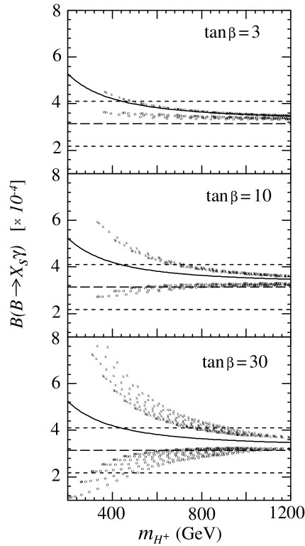
FIG. 12.: $B(B\to X_{s}\gamma)$, including standard model, $H^{\pm}$, and SUSY contributions, as a function of $m_{H^{\pm}}$ for $\mu>0$ ($\times$) and $\mu<0$ ($\circ$) and three representative values of $\tan\beta$. Also shown are the theoretical prediction including only the $H^{\pm}$ contribution (solid), and the current experimental value and $2\sigma$ experimental limits (dashed).

As in minimal supergravity and gauge-mediated models, the neutralino diagrams are negligible, but the chargino and, to a lesser extent, gluino diagrams may be substantial, especially for large $\tan\beta$. In contrast to these other SUSY models, however, as a result of the sign flips in $A_{t}$ and $M_{3}$ noted above, both chargino and gluino contributions enhance the standard model prediction for $\mu>0$. The parameter space with $\mu>0$ is thus highly constrained, and requires large charged Higgs masses, especially for large $\tan\beta$. For example, for $\tan\beta=30$, the upper bound of Eq. (40) implies $m_{H^{\pm}}\gtrsim 700\text{ GeV}$, significantly more stringent than the bound $m_{H^{\pm}}\gtrsim 400\text{ GeV}$ that would apply in the absence of chargino and gluino contributions. For $\mu<0$, the supersymmetric contributions may cancel the charged Higgs contribution, and the parameter space is constrained only for very low $M_{\text{aux}}$ and $m_{0}$, where the destructive SUSY contributions push $B(B\to X_{s}\gamma)$ below experimental bounds.

In Figs. 13 and 14 we plot $B(B\to X_{s}\gamma)$ in the $(m_{0},M_{\text{aux}})$ plane for various values of $\tan\beta$ and $\>\!\text{sign}\>\!(\mu)$. Regions excluded by Eq. (40) are shaded; for $\mu>0$ and large $\tan\beta$, this includes much of the parameter space with light sleptons and light Winos.

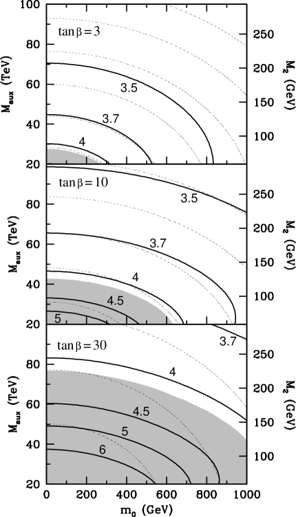
FIG. 13.: $B(B\to X_{s}\gamma)$ ($\times 10^{-4}$) (solid) for $\mu>0$ and three representative values of $\tan\beta$. For reference, also shown are contours of constant $m_{H^{\pm}}=500,750,1000,\cdots$ GeV, from the lower left (dotted). The shaded region is excluded by $B(B\to X_{s}\gamma)<4.10\times 10^{-4}$.

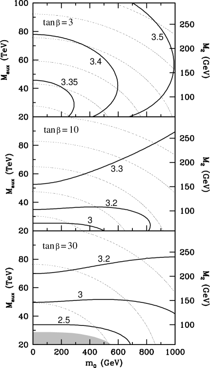
FIG. 14.: Contours as in Fig. 13, but for $\mu<0$. The shaded region is excluded by $B(B\to X_{s}\gamma)>2.18\times 10^{-4}$.

B Muon magnetic dipole moment

While anomaly-mediated SUSY breaking does not contribute substantially to flavor-violating observables involving the first and second generations, it may give significant contributions to flavor-conserving observables involving the first and second generations. It is well-known that SUSY loops may give a sizable contribution to the muon magnetic dipole moment (MDM) [38]. The SUSY contribution to the muon MDM is from smuon-neutralino and sneutrino-chargino loop diagrams. Since these superparticles may have masses comparable to the electroweak scale, these contributions may be comparable to, or even larger than, electroweak contributions from $W$- and $Z$-boson diagrams. The on-going Brookhaven E821 experiment [39] is expected to measure the muon MDM with an accuracy of $0.4\times 10^{-9}$, which is about a few times smaller than the electroweak contribution to the muon MDM. Therefore, the Brookhaven E821 experiment will provide an important constraint on SUSY models.

In general, the muon anomalous MDM is given by the coefficient of the “magnetic moment-type” operator

$${\cal L}_{\rm MDM}=\frac{e}{4m_{\mu}}a_{\mu}\bar{\mu}\sigma_{\mu\nu}\mu F_{\mu\nu}\ ,$$ (41)

where the anomalous magnetic moment $a_{\mu}$ is related to the muon $g-2$ by $a_{\mu}=\frac{1}{2}(g-2)_{\mu}$.

As suggested from the structure of the operator, diagrams for the muon anomalous MDM require a left-right muon transition. In SUSY diagrams, this transition may occur through a chirality flip along the external muon line, through left-right mixing in the smuon mass matrix, or through the interaction of a muon and smuon with a Higgsino. In the latter two cases, the diagrams are proportional to the muon Yukawa coupling constant and are therefore enhanced for large $\tan\beta$. These diagrams also include gaugino mass insertions. As a result, in the large $\tan\beta$ limit, the muon anomalous MDM is given by

$$a_{\mu}^{\rm SUSY} \simeq \frac{g_{1}^{2}}{16\pi^{2}}m_{\mu}^{2}\mu M_{1}\tan\beta\times F_{1}(m_{\tilde{\mu}}^{2},m_{\tilde{\chi}^{0}}^{2})$$ (43)

$$+\frac{g_{2}^{2}}{16\pi^{2}}m_{\mu}^{2}\mu M_{2}\tan\beta\times F_{2}(m_{\tilde{\mu}}^{2},m_{\tilde{\nu}}^{2},m_{\tilde{\chi}^{0}}^{2},m_{\tilde{\chi}^{\pm}}^{2})\ ,$$

where the $F$ functions (see the last reference in Ref. [38]) are typically $F\sim m_{\rm SUSY}^{-4}$, with $m_{\rm SUSY}$ being the mass scale of the superparticles in the loop. For large $\tan\beta$, then, the SUSY contribution $a_{\mu}^{\rm SUSY}$ is approximately proportional to $\tan\beta$ and may be much larger than the electroweak contribution.

Results for the SUSY contribution to the muon MDM $a_{\mu}^{\rm SUSY}$ in the minimal anomaly-mediated model are given in Fig. 15.

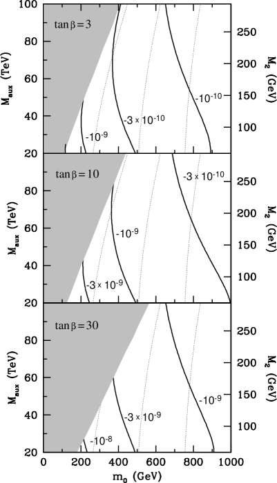
FIG. 15.: The muon anomalous magnetic moment $a_{\mu}^{\text{SUSY}}=\frac{1}{2}(g-2)^{\text{SUSY}}_{\mu}$ (solid) in the $(m_{0},M_{\text{aux}})$ plane for $\mu<0$ and three representative values of $\tan\beta$. Also shown are contours of constant $m_{\tilde{\mu}}=250$, 500, and 750 GeV from the left (dotted). The shaded region is excluded by $m_{\tilde{\tau}_{1}}>70\text{ GeV}$. Results for $\mu>0$ are of similar magnitude, but opposite in sign.

Both $\tan\beta$ enhanced and unenhanced contributions were included by using the mass eigenstate bases of squarks, sleptons, neutralinos, and charginos. The SUSY contribution to the muon MDM is typically $\sim 10^{-8}-10^{-10}$, and is enhanced for large $\tan\beta$. Furthermore, heavier superparticles suppress $a_{\mu}^{\rm SUSY}$, as expected.

Experimentally, the muon anomalous MDM is currently constrained to be [40]

$$a_{\mu}^{\rm exp}=(1~{}165~{}923.0\pm 8.4)\times 10^{-9}\ ,$$ (44)

and hence the anomaly-mediated SUSY contribution is usually smaller than the present experimental accuracy, unless $\tan\beta$ is very large. However, as mentioned above, in the near future, the Brookhaven E821 experiment will improve the measurement, with a projected error of $0.4\times 10^{-9}$. If this is realized, some anomaly may be seen in the muon MDM in the anomaly-mediated SUSY breaking scenario, particularly for moderate or large values of $\tan\beta$.

C Electric dipole moments of the electron and neutron

In general, parameters in SUSY models are complex, and (some combinations of) their phases are physical. In the anomaly-mediated SUSY breaking scenario, most of the SUSY breaking parameters are proportional to the single parameter $M_{\text{aux}}$, and so many of the phases can be rotated away. In particular, the gaugino mass parameters and the $A$ parameters can be made real simultaneously. However, even in anomaly-mediated SUSY breaking, a physical phase may exist in the $\mu$ and $B_{\mu}$ parameters since their origins are not well-understood. In our analysis, we have not assumed any relation between $\mu$ and $B_{\mu}$, and have simply constrained them so that electroweak symmetry is properly broken. In this approach, one physical phase remains, which is given by

$$\theta_{\rm phys}\equiv{\rm Arg}(\mu B^{*}_{\mu}M_{i})\ .$$ (45)

If this phase is non-vanishing, electric dipole moments (EDMs) are generated. As is known from general analyses, the EDMs of the electron and neutron may be extremely large unless $|\sin\theta_{\rm phys}|$ is suppressed [41].

To determine the constraints on this phase in the anomaly-mediated framework, we calculate the electron and neutron EDMs with the minimal anomaly-mediated model mass spectrum. The EDM $d_{f}$ of a fermion $f$ is given by the effective electric dipole interaction

$${\cal L}_{\rm EDM}=-\frac{i}{2}d_{f}\bar{f}\sigma_{\mu\nu}\gamma_{5}fF_{\mu\nu}\ ,$$ (46)

which becomes ${\cal L}_{\rm EDM}\simeq d_{f}\vec{\sigma}\cdot\vec{E}$ in the non-relativistic limit.

The calculation of the electron EDM is similar to that of the muon anomalous MDM, since the structure of the Feynman diagrams is almost identical. If the slepton masses are flavor universal, $a_{\mu}$ and $d_{e}$ are approximately related by

$$d_{e}\simeq\frac{m_{e}}{2m_{\mu}^{2}}\tan\theta_{\rm phys}\times a^{\rm SUSY}_{\mu}\ ,$$ (47)

Therefore, the electron EDM is also proportional to $\tan\beta$.

The calculation of the up and down quark EDMs is also straightforward, given the SUSY model parameters. The only major difference from the electron EDM is the contribution from the squark-gluino diagram. However, in calculating the neutron EDM, we must adopt some model for the structure of the neutron. We use the simplest model, i.e., the non-relativistic quark model. The neutron EDM is then given by

$$d_{n}=\frac{1}{3}(4d_{d}-d_{u})\ .$$ (48)

Since $d_{d}$ is also proportional to $\tan\beta$, the neutron EDM is also enhanced for large $\tan\beta$.

Figures 16 and 17 show the EDMs of the electron and neutron, respectively, in the minimal anomaly-mediated model. The EDMs are proportional to $\sin\theta_{\rm phys}$. In these plots, we assume maximal CP violation, i.e., $\sin\theta_{\rm phys}=1$.

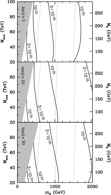
FIG. 16.: The electric dipole moment of the electron $|d_{e}|$ in units of $e$-cm in the $(m_{0},M_{\text{aux}})$ plane, assuming $\sin\theta_{\rm phys}=1$, for $\mu<0$ and three representative values of $\tan\beta$. Also shown are contours of constant $m_{\tilde{e}}=250$, 500, and 750 GeV from the left (dotted). The shaded region is excluded by $m_{\tilde{\tau}_{1}}>70\text{ GeV}$.

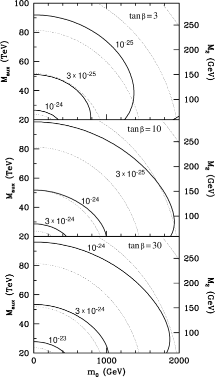
FIG. 17.: The electric dipole moment of the neutron $|d_{n}|$ in units of $e$-cm in the $(m_{0},M_{\text{aux}})$ plane, assuming $\sin\theta_{\rm phys}=1$, for $\mu<0$ and three representative values of $\tan\beta$. Also shown are contours of constant $m_{\tilde{u}_{L}}=500$, 1000,$\cdots$, 2500 GeV, from the lower left (dotted).

Currently, there is no experimental result which suggests a non-vanishing EDM, and experimental constraints on the EDMs are very stringent. For the electron EDM, using $d_{e}=(0.18\pm 0.12\pm 0.10)\times 10^{-26}e$ cm [42], we obtain the constraint

$$|d_{e}|\leq 0.44\times 10^{-26}e~{}{\rm cm}\ ,$$ (49)

where the right-hand side is the upper bound on $d_{e}$ at 90% C.L. For the neutron, $d_{n}$ is constrained to be [40]

$$|d_{n}|\leq 0.97\times 10^{-25}e~{}{\rm cm}\ .$$ (50)

The naturalness arguments of Sec. IV play an important part in evaluating the sensitivity of the EDMs. For $d_{e}$ and small $\tan\beta$, while very large effects are possible, $d_{e}$ may be within the experimental bounds even for $|\sin\theta_{\rm phys}|$ close to 1 without violating the condition $|\mu|\lesssim 1\text{ TeV}$. For moderate and large $\tan\beta$, $d_{e}$ becomes much larger, and the physical phase $\theta_{\rm phys}$ is constrained to be $|\sin\theta_{\rm phys}|\lesssim{\cal O}(10^{-2})$ for $m_{0}\approx 1\text{ TeV}$. However, for such $\tan\beta$, the naturalness bound on $m_{0}$ is also relaxed, and reasonably large ${\cal O}(0.1)$ phases are possible in natural regions of parameter space where $d_{e}$ is suppressed by slepton masses of a few TeV. Thus, while large effects comparable to current bounds are predicted in much of parameter space, constraints from $d_{e}$ may also be satisfied by superpartner decoupling in the minimal anomaly-mediated model. For $d_{n}$, similar conclusions hold. In fact, the constraints from $d_{n}$ on the CP-violating phases are more easily satisfied, and $d_{e}$ appears to be the more stringent constraint at present.

In our discussion, as noted above, we have not assumed a specific model for the $\mu$ and $B_{\mu}$ parameters, and hence we regarded $\theta_{\rm phys}$ as a free parameter. However, several mechanisms have been proposed to generate $\mu$ and $B_{\mu}$ in which $\sin\theta_{\rm phys}$ vanishes [3, 7, 9]. In those scenarios, of course, $d_{e}$ and $d_{n}$ vanish, and the EDM constraints are automatically satisfied.

VII Conclusions

In this study we have analyzed a model of “supernatural supersymmetry,” in which squarks and sleptons may be much heavier than their typical naturalness limits, and SUSY is broken in another world. SUSY breaking is then communicated to our world dominantly via anomaly-mediation, and we have considered in detail a model in which tachyonic sleptons are avoided by a non-anomaly-mediated universal scalar mass $m_{0}$.

The novel naturalness properties of this model are a result of a “focus point” behavior in the RG evolution of $m_{H_{u}}^{2}$, such that its weak scale value is highly insensitive to $m_{0}$. Naturalness bounds on superparticle masses are therefore highly variable and differ from naive expectations. Naturalness places strong bounds on gaugino masses, and Wino masses $M_{2}\lesssim 200\text{ GeV}$ are preferred. On the other hand, for moderate and large values of $\tan\beta$, multi-TeV values of $m_{0}$, and therefore slepton and squark masses, are natural.

A number of spectacular collider signals are possible. The possibility of a highly degenerate triplet of Wino LSPs has recently attracted a great deal of attention [5, 6, 15, 16, 17]. In the minimal anomaly-mediated scenario, we find that Winos are not only the LSPs in much of parameter space, but are typically light, with mass $\lesssim 200\text{ GeV}$, and extraordinarily degenerate, with charged Wino decay lengths of several centimeters. Such Wino characteristics are ideal for Tevatron searches, where Winos may appear as vertex detector track stubs in monojet events. The prospects for discovery at the Tevatron in Run II or III are highly promising [5].

In the remaining parameter space, the LSP is either the lighter stau, or the tau sneutrino. In the $\tilde{\tau}_{1}$ LSP scenario, the $\tilde{\tau}_{1}$ is typically lighter than 200 GeV and is stable. It may be found in searches for stable charged massive particles at both LEP [19] and the Tevatron [22, 24, 25]. In the $\tilde{\nu}_{\tau}$ LSP scenario, the Winos, $\tilde{\tau}_{1}$ and sneutrinos are all $\lesssim 110\text{ GeV}$. In both scenarios, ongoing searches at LEP and the Tevatron will be able to probe substantial portions of the relevant parameter space.

The minimal anomaly-mediated model also has a number of other features that distinguish it from other models. In addition to characteristic gaugino mass ratios, these include highly degenerate same-flavor sleptons, and large left-right mixing. If SUSY is discovered, measurements of slepton masses and mixings will provide strong evidence for or against the minimal model and its assumption of an additional universal slepton mass.

We have also considered a variety of low energy observables that are sensitive probes of anomaly-mediated parameter space. Effects on the flavor-changing process $b\to s\gamma$ may be large, and significant regions of parameter space for large $\tan\beta$ and $\mu>0$ are already excluded. The anomalous magnetic moment of the muon may also be affected at levels soon to be probed by experiment. Finally, the electron and neutron electric dipole moments provide rather strong constraints on the CP-violation phase $\theta_{\text{phys}}$ in much of parameter space, but even for large $\tan\beta$, ${\cal O}(0.1)$ phases are still be allowed for multi-TeV $m_{0}$ at its focus point naturalness limit.

It is interesting to note that positive signals in these low energy experiments may not only provide evidence for SUSY, but may also exclude some supersymmetric interpretations and favor others. For example, the signs of the SUSY contributions to $b\to s\gamma$ and $a_{\mu}^{\rm SUSY}$ are determined by $\>\!\text{sign}\>\!(\mu M_{3})$  and $\>\!\text{sign}\>\!(\mu M_{2})$, respectively. A large anomalous measurement of $a_{\mu}^{\rm SUSY}$ would imply large $\tan\beta$, and, given the current bounds on $b\to s\gamma$, a preferred sign for $\>\!\text{sign}\>\!(\mu M_{3})$. The sign of the $a_{\mu}^{\rm SUSY}$ anomaly then determines $\>\!\text{sign}\>\!(M_{2}M_{3})$. For example, assuming a SUSY interpretation, a large negative anomalous MDM measurement would imply $M_{2}M_{3}<0$, and would favor anomaly-mediated models over virtually all other well-motivated models.

Finally, as stated in Sec. III, the assumption of a universal scalar mass contribution, while possibly generated by bulk contributions [3], does not hold generally in anomaly-mediated scenarios. Several features presented above depend on various parts of this assumption, and we therefore close with a brief discussion of these dependences.

The naturalness properties described above, and, in particular, the focus point behavior, results from the fact that the non-anomaly-mediated piece is identical for $m_{H_{u}}^{2}$, $m_{U_{3}}^{2}$, and $m_{Q_{3}}^{2}$. While the focus point mechanism as implemented here relies on this subset of the universal boundary conditions, a variety of other boundary conditions also have similar properties, and it would be interesting to explore applications of the focus point mechanism in other settings. The accidental degeneracy of left- and right-handed sleptons, and the possibility for large left-right mixings, holds only if both left- and right-handed sleptons receive the same non-anomaly-mediated contribution. Measurement of large left-right smuon mixing, along with confirmation of anomaly-mediated gaugino mass parameters, for example, would therefore be strong evidence for anomaly-mediation with a universal slepton mass contribution. Finally, the low energy observables discussed are sensitive quantitatively to either the hadronic or leptonic superpartner spectrum. However, qualitative results, such as the stringency of constraints for large $\tan\beta$, can be expected to remain valid for a variety of anomaly-mediated models, as long as the attractive flavor properties of anomaly-mediation are preserved in these models and they do not have new large sources of flavor violation.

Anomaly-Mediated Boundary Conditions

In this appendix, we present the leading order soft supersymmetry breaking terms, first for a general anomaly-mediated supersymmetric theory, and then for the minimal anomaly-mediated model.

Consider a supersymmetric theory with simple gauge group $G$. The anomaly-mediated boundary conditions are completely specified in terms of the gauge coupling $g$, supersymmetric Yukawa couplings

$$W=\frac{1}{6}Y^{ijk}\phi_{i}\phi_{j}\phi_{k}\ ,$$ (51)

and the supersymmetry breaking parameter $M_{\text{aux}}$.

In the convention that the soft supersymmetry-breaking terms are

$${\cal L_{\text{SSB}}}=-\frac{1}{2}M_{\lambda}(-i\lambda)(-i\lambda)-\frac{1}{2}(m^{2})_{i}^{j}\tilde{\phi}^{\ast i}\tilde{\phi}_{j}-\frac{1}{6}A^{ijk}\tilde{\phi}_{i}\tilde{\phi}_{j}\tilde{\phi}_{k}\ ,$$ (52)

the leading order anomaly-mediated soft supersymmetry breaking terms are

$$M_{\lambda}|_{\rm AM} = \frac{1}{16\pi^{2}}bg^{2}M_{\rm aux}$$ (53)

$${(m^{2})}_{i}^{j}|_{\rm AM} = \frac{1}{2}\left(\dot{\gamma}\right)_{i}^{j}M_{\rm aux}^{2}$$ (54)

$$A^{ijk}|_{\rm AM} = -\sum_{m}\left(Y^{mjk}\gamma_{m}^{i}+Y^{imk}\gamma_{m}^{j}+Y^{ijm}\gamma_{m}^{k}\right)M_{\rm aux}\ ,$$ (55)

where

$$\gamma_{i}^{j}=\frac{1}{2}Y_{imn}Y^{jmn}-2\delta_{i}^{j}g^{2}C(i)\ .$$ (56)

Here $\dot{(\ )}\equiv d/d\ln\mu$, $Y_{ijk}={Y^{ijk}}^{\ast}$, and the one-loop $\beta$-function coefficient is $b=S(R)-3C(G)$, where $C(i)$ is the quadratic Casimir invariant for representation $i$, and $S(R)$ is the total Dynkin index summed over all the chiral superfields. In terms of the matter field wavefunction $Z$, $\gamma_{i}^{j}\equiv-\frac{1}{2}\dot{\left(\ln Z\right)}_{i}^{j}$.

For minimal field content, anomaly-mediated gaugino masses are given as

$$M_{i}=\frac{1}{16\pi^{2}}b_{i}g_{i}^{2}M_{\rm aux}\ ,$$ (57)

where $b_{i}=(\frac{33}{5},1,-3)$ in the GUT normalization. Furthermore, with the superpotential

$$W=U_{i}\mbox{\boldmath$Y_{u}$}_{ij}Q_{j}H_{u}+D_{i}\mbox{\boldmath$Y_{d}$}_{ij}Q_{j}H_{d}+E_{i}\mbox{\boldmath$Y_{e}$}_{ij}L_{j}H_{d}\ ,$$ (58)

the flavor-dependent wavefunction factors are

$$16\pi^{2}\gamma_{H_{u}} = 3\>\!\text{Tr}\>\!(\mbox{\boldmath$Y_{u}$}^{\dagger}\mbox{\boldmath$Y_{u}$})-\frac{3}{2}g_{2}^{2}-\frac{3}{10}g_{1}^{2}$$ (59)

$$16\pi^{2}\gamma_{H_{d}} = 3\>\!\text{Tr}\>\!(\mbox{\boldmath$Y_{d}$}^{\dagger}\mbox{\boldmath$Y_{d}$})+\>\!\text{Tr}\>\!(\mbox{\boldmath$Y_{e}$}^{\dagger}\mbox{\boldmath$Y_{e}$})-\frac{3}{2}g_{2}^{2}-\frac{3}{10}g_{1}^{2}$$ (60)

$$16\pi^{2}\mbox{\boldmath$\gamma_{Q}$} = \mbox{\boldmath$Y_{u}$}^{\dagger}\mbox{\boldmath$Y_{u}$}+\mbox{\boldmath$Y_{d}$}^{\dagger}\mbox{\boldmath$Y_{d}$}-\frac{8}{3}g_{3}^{2}-\frac{3}{2}g_{2}^{2}-\frac{1}{30}g_{1}^{2}$$ (61)

$$16\pi^{2}\mbox{\boldmath$\gamma_{U}$} = 2\mbox{\boldmath$Y_{u}$}^{*}\mbox{\boldmath$Y_{u}$}^{T}-\frac{8}{3}g_{3}^{2}-\frac{8}{15}g_{1}^{2}$$ (62)

$$16\pi^{2}\mbox{\boldmath$\gamma_{D}$} = 2\mbox{\boldmath$Y_{d}$}^{*}\mbox{\boldmath$Y_{d}$}^{T}-\frac{8}{3}g_{3}^{2}-\frac{2}{15}g_{1}^{2}$$ (63)

$$16\pi^{2}\mbox{\boldmath$\gamma_{L}$} = \mbox{\boldmath$Y_{e}$}^{\dagger}\mbox{\boldmath$Y_{e}$}-\frac{3}{2}g_{2}^{2}-\frac{3}{10}g_{1}^{2}$$ (64)

$$16\pi^{2}\mbox{\boldmath$\gamma_{E}$} = 2\mbox{\boldmath$Y_{e}$}^{*}\mbox{\boldmath$Y_{e}$}^{T}-\frac{6}{5}g_{1}^{2}\ ,$$ (65)

where the Yukawa couplings $Y$ are $3\times 3$ matrices in generation space.

The gauge and Yukawa coupling RG equations are as in Ref. [43], and are reproduced here for convenience and completeness:

$$16\pi^{2}\dot{g}_{i} = b_{i}g_{i}^{3}$$ (66)

$$16\pi^{2}\dot{\mbox{\boldmath$Y_{u}$}} = \mbox{\boldmath$Y_{u}$}\left[3\>\!\text{Tr}\>\!(\mbox{\boldmath$Y_{u}$}\mbox{\boldmath$Y_{u}$}^{\dagger})+3\mbox{\boldmath$Y_{u}$}^{\dagger}\mbox{\boldmath$Y_{u}$}+\mbox{\boldmath$Y_{d}$}^{\dagger}\mbox{\boldmath$Y_{d}$}-\frac{16}{3}g_{3}^{2}-3g_{2}^{2}-\frac{13}{15}g_{1}^{2}\right]$$ (67)

$$16\pi^{2}\dot{\mbox{\boldmath$Y_{d}$}} = \mbox{\boldmath$Y_{d}$}\left[3\>\!\text{Tr}\>\!(\mbox{\boldmath$Y_{d}$}\mbox{\boldmath$Y_{d}$}^{\dagger})+3\>\!\text{Tr}\>\!(\mbox{\boldmath$Y_{e}$}\mbox{\boldmath$Y_{e}$}^{\dagger})+3\mbox{\boldmath$Y_{d}$}^{\dagger}\mbox{\boldmath$Y_{d}$}+\mbox{\boldmath$Y_{u}$}^{\dagger}\mbox{\boldmath$Y_{u}$}-\frac{16}{3}g_{3}^{2}-3g_{2}^{2}-\frac{7}{15}g_{1}^{2}\right]$$ (68)

$$16\pi^{2}\dot{\mbox{\boldmath$Y_{e}$}} = \mbox{\boldmath$Y_{e}$}\left[3\>\!\text{Tr}\>\!(\mbox{\boldmath$Y_{d}$}\mbox{\boldmath$Y_{d}$}^{\dagger})+\>\!\text{Tr}\>\!(\mbox{\boldmath$Y_{e}$}\mbox{\boldmath$Y_{e}$}^{\dagger})+3\mbox{\boldmath$Y_{e}$}^{\dagger}\mbox{\boldmath$Y_{e}$}-3g_{2}^{2}-\frac{9}{5}g_{1}^{2}\right]\ .$$ (69)

Our sign convention for the $\mu$ and $A$ parameters is such that, with soft terms as defined in Eq. (52), the chargino mass terms are $(\psi^{-})^{T}\mbox{\boldmath$M_{\tilde{\chi}^{\pm}}$}\psi^{+}+{\rm h.c.}$, where $(\psi^{\pm})^{T}=(-i\tilde{W}^{\pm},\tilde{H}^{\pm})$ and

$$\mbox{\boldmath$M_{\tilde{\chi}^{\pm}}$}=\left(\begin{array}[]{cc}M_{2}&\sqrt{2}\,m_{W}\sin\beta\\ \sqrt{2}\,m_{W}\cos\beta&\mu\end{array}\right)\ ,$$ (70)

and the stop left-right mixing terms are $m_{t}(A_{t}-\mu\cot\beta)$.

REFERENCES

- [1] F. Gabbiani, E. Gabrielli, A. Masiero and L. Silvestrini, Nucl. Phys. B477, 321 (1996).
- [2] M. Dine and A. E. Nelson, Phys. Rev. D48, 1277 (1993); M. Dine, A. E. Nelson, and Y. Shirman, Phys. Rev. D51, 1362 (1995); 1362 (1995); M. Dine, A. E. Nelson, Y. Nir, and Y. Shirman, Phys. Rev. D53, 2658 (1996).
- [3] L. Randall and R. Sundrum, hep-th/9810155;
- [4] G. Giudice, M. Luty, H. Murayama, and R. Rattazzi, JHEP 9812, 027 (1998).
- [5] J. L. Feng, T. Moroi, L. Randall, M. Strassler, and S. Su, to appear in Phys. Rev. Lett., hep-ph/9904250.
- [6] T. Gherghetta, G. Giudice, and J. Wells, hep-ph/9904378.
- [7] A. Pomarol and R. Rattazzi, JHEP 9905, 013 (1999).
- [8] Z. Chacko, M. A. Luty, I. Maksymyk, and E. Ponton, hep-ph/9905390.
- [9] E. Katz, Y. Shadmi, and Y. Shirman, hep-ph/9906296.
- [10] T. Moroi and L. Randall, hep-ph/9906527.
- [11] I. Jack and D. R. T. Jones, hep-ph/9907255.
- [12] M. Drees and M. M. Nojiri, Phys. Rev. D45, 2482 (1992).
- [13] See, e.g., G. W. Anderson and D. J. Castano, Phys. Lett. B347, 300 (1995); ibid., Phys. Rev. D52, 1693 (1995); and references therein.
- [14] See, for example, M. Wise, in Proceedings of TASI ’87, edited by R. Slansky and G. West (World Scientific, Singapore, 1988); J. Bagger, in Proceedings of TASI ’95, edited by D. Soper (World Scientific, Singapore, 1996), pp. 109-162; J. L. Feng, C. Kolda, and N. Polonsky, Nucl. Phys. B546, 3 (1999); J. Bagger, J. L. Feng, and N. Polonsky, hep-ph/9905292.
- [15] C.-H. Chen, M. Drees, and J. F. Gunion, Phys. Rev. Lett. 76, 2002 (1996); ibid., Phys. Rev. D55, 330 (1997); Erratum, hep-ph/9902309.
- [16] H.-C. Cheng, B. A. Dobrescu, and K. T. Matchev, Nucl. Phys. B543, 47 (1999).
- [17] J. F. Gunion and S. Mrenna, hep-ph/9906270.
- [18] S. Thomas and J. D. Wells, Phys. Rev. Lett. 81, 34 (1998).
- [19] Delphi Collaboration, hep-ex/9903071.
- [20] The SUSY Working Group, J. Bagger et al., in Proceedings of the 1996 DPF/DPB Summer Study on New Directions for High Energy Physics (Snowmass 96), June 25 – July 12, 1996, pp. 642–654, hep-ph/9612359.
- [21] M. M. Nojiri, Phys. Rev. D51, 6281 (1995); M. M. Nojiri, K. Fujii, and T. Tsukamoto, Phys. Rev. D54, 6756 (1996).
- [22] LEP SUSY Working Group, ALEPH, DELPHI, L3 and OPAL experiments, note LEPSUSYWG/99-01.1.
- [23] J. Ellis, T. Falk, K. A. Olive, and M. Schmitt, Phys. Lett. B388, 97 (1996).
- [24] M. Drees and X. Tata, Phys. Lett. B252, 695 (1990); J. L. Feng and T. Moroi, Phys. Rev. D58, 035001 (1998); S. P. Martin and J. D. Wells, Phys. Rev. D59, 035008 (1999).
- [25] D. Stuart, private communication; K. Hoffman for the CDF and DØCollaborations, talk presented at HEP 97, Jerusalem, Israel, August 19–26, 1997, hep-ex/9712032; D. Cutts and G. Landsberg, hep-ph/9904396.
- [26] M. Dine, L. Randall, and S. Thomas, Phys. Rev. Lett. 75, 398 (1995); D. H. Lyth and E. D. Stewart, Phys. Rev. Lett. 75, 201 (1995); ibid., Phys. Rev. D53, 1784 (1996).
- [27] For recent analyses, see, e.g., E. Gabrielli and U. Sarid, Phys. Rev. D58, 115003 (1998); T. Goto, Y. Okada, and Y. Shimizu, Phys. Rev. D58, 094006 (1998).
- [28] K. Adel and Y. P. Yao, Phys. Rev. D49, 4945 (1994); C. Greub and T. Hurth, Phys. Rev. D56, 2934 (1997); A. J. Buras, A. Kwiatkowski, and N. Pott, Phys. Lett. B414, 157 (1997); ibid., Nucl. Phys. B517, 353 (1998).
- [29] M. Ciuchini, G. Degrassi, P. Gambino, and G. F. Giudice, Nucl. Phys. B527, 21 (1998); F. Borzumati and C. Greub, Phys. Rev. D58, 074004 (1998); ibid., Phys. Rev. D59, 057501 (1999); ibid., hep-ph/9810240.
- [30] S. Bertolini, F. Borzumati, A. Masiero, and G. Ridolfi, Nucl. Phys. B353, 591 (1991).
- [31] M. Ciuchini, G. Degrassi, P. Gambino, and G. F. Giudice, Nucl. Phys. B534, 3 (1998); C. Bobeth, M. Misiak, and J. Urban, hep-ph/9904413.
- [32] K. Chetyrkin, M. Misiak, and M. Münz, Phys. Lett. B400, 206 (1997); Erratum, 425, 414 (1998);
- [33] A. Ali and C. Greub, Phys. Lett. B361, 146 (1995); C. Greub, T. Hurth, and D. Wyler, Phys. Lett. B380, 385 (1996); ibid., Phys. Rev. D54, 3350 (1996); N. Pott, Phys. Rev. D54, 938 (1996).
- [34] A. Strumia, Nucl. Phys. B532, 28 (1998); A. Czarnecki and W. J. Marciano, Phys. Rev. Lett. 81, 277 (1998);
- [35] A.L. Kagan and M. Neubert, Eur. Phys. J. C7, 5 (1999).
- [36] CLEO Collaboration, S. Glenn et al., CLEO–CONF 98–17, ICHEP98 1011; J. Alexander, in the proceedings of the 29th International Conference on High-Energy Physics (ICHEP 98), Vancouver, Canada, 23-29 July 1998.
- [37] ALEPH Collaboration, R. Barate et al., Phys. Lett. B429, 169 (1998).
- [38] See, for example, J. Lopez, D. V. Nanopoulos, and X. Wang, Phys. Rev. D49, 366 (1991); U. Chattopadhyay and P. Nath, Phys. Rev. D53, 1648 (1996); M. Carena, G. F. Giudice, and C. E. M. Wagner, Phys. Lett. B390, 234 (1997); T. Moroi, Phys. Rev. D53, 6565 (1996); Erratum, D56 (1997) 4424; and references therein.
- [39] T. Kinoshita, in Frontiers of High Energy Spin Physics, edited by T. Hasegawa et al. (Universal Academy Press, 1993), p. 9.
- [40] The Particle Data Group, C. Caso et al., Eur. Phys. J. C3, 1 (1998).
- [41] See, for example, P. Nath, Phys. Rev. Lett. 66, 2565 (1991); Y. Kizukuri and N. Oshimo, Phys. Rev. D46, 3025 (1992); M. Brhlik, G. J. Good, and G. L. Kane, Phys. Rev. D59, 115004 (1999); T. Moroi, Phys. Lett. B447, 75 (1999); and references therein.
- [42] E. D. Commins, S. B. Ross, D. DeMille, and B. C. Regan, Phys. Rev. A50, 2960 (1994).
- [43] S. P. Martin and M. T. Vaughn, Phys. Rev. D50, 2282 (1994).