IUHET-415

Abstract

We make a comprehensive analysis of an extended supersymmetric model(ESSM) obtained by adding a pair of vector-like families to the minimal supersymmetric standard model and having specific forms of $5\times 5$ fermion mass matrices. The singlet Higgs couplings which link the ordinary to vector-like generations do not have the renormalization effects of the gauge interactions and hence the “quasi-infrared fixed point” near the scale of the top quark mass. The two-loop Yukawa effects on gauge couplings lead to an unified coupling $\alpha_{X}$ around $0.2$ with an unification scale $M_{X}$ of $10^{16.9}$ GeV. Large Yukawa effects in the high energy region arrest the growth of the QCD coupling near $M_{X}$ making the evolution flat. The renormalization effects of the vector-like generations on soft mass parameters has important effects on the charge and color breaking(CCB)minima. We will show that there exists parameter space where there is no charge and color breaking. We will also demonstrate that there exists minima of the Higgs potential which satisfies the mass of the Z boson but avoid CCB. Upper limits on the mass of the lightest Higgs boson from the one-loop effective scalar potential is obtained for sets of universal soft supersymmetry breaking mass parameters.

1 Introduction

The commonly accepted notion of a unified coupling $\alpha_{X}=0.04$ at $10^{16}$ GeV has been questioned recently in view of a conjecture that the four dimensional unified string coupling is likely to have a semi-perturbative value (0.2-0.3) at the string unification scale (see later) so that it may be large enough to stabilize the dilaton but not as large as to ruin the supersymmetric gauge coupling unification[1].

It may be noted that the MSSM unification scale $M_{X}=2\times 10^{16}$ GeV appears to be a factor of 20 smaller than the one-loop level string unification scale of $M_{st}\sim g_{st}~{}5.2\times 10^{17}~{}{\rm GeV}\sim 3.6\times 10^{17}$ GeV[2, 3]. In this context the extensions of MSSM spectrum addressing the issues of $\alpha_{X}$ and $M_{X}$ may be interesting. The specific extension which we will consider is called as the Extended Supersymmetric Standard Model (ESSM). This itinerary extends the MSSM particle spectrum by adding two light vector-like families which are $Q_{L,R}=(U,D,N,E)_{L,R}$ and $Q^{\prime}_{L,R}=(U^{\prime},D^{\prime},N^{\prime},E^{\prime})_{L,R}$ and two Higgs singlet scalars $H_{S}$ and $H_{\lambda}$. These new particles and as well as their superpartners are 1 to a few TeVs[1]. ESSM has no unified gauge group as such and so the corresponding leptoquark and di-quark gauge bosons leading to proton decay does not exist. The extra sets of matter fields denoted by previous authors $Q_{L}|{\overline{Q}^{\prime}_{R}}$ and $\overline{Q_{R}}|Q^{\prime}_{L}$ can be thought of as ${16}$ and ${\overline{16}}$ representations of a cosmetic unified gauge group of SO(10).

It has been noted sometime ago that precision measurements of the oblique electroweak parameters and the number of light neutrino species $N_{\nu}$ does not favor extra chiral families. They do not however constrain vector-like families due to decoupling effects[4, 5]. Such vector-like families i.e., ${16}$ and ${\overline{16}}$, which apparently are predicted generically in string theories could well exist in the TeV region. It may be worth understanding that the pair of vector-like families could give us a clue to the family mass hierarchy within the three chiral generations via a see-saw mechanism residing inside the $5\times 5$ fermion mass matrices[6].

Such a pair of vector-like families and thus ESSM provide some unique advantages over MSSM. They are as follows.

$\bullet$ One-loop evolution of three gauge couplings maintains the approximate meeting when complete extra families such as vector-like families are included.

$\bullet$ Although one-loop approximation leads to the unification of the three $\alpha_{i}$’s at the same scale $M_{X}$ the unified coupling $\alpha_{X}$ increases.

$\bullet$ Numerically speaking $\alpha_{X}$ can be raised to $0.2-0.3$ in one loop. Two-loop gauge couplings accelerate the growth whereas the two loop Yukawa effects on gauge couplings does the contrary. This is vital for having a good fit to $\alpha_{s}(m_{Z})$ within unification.

Now we briefly describe the work of the previous authors[1]. Instead of using the $\theta$ function approximation to study the particle thresholds they used exact threshold functions [7, 8]. The evolution of the Yukawa couplings was studied in one-loop. The off-diagonal Yukawa couplings between the third family and the vector-like families and the self couplings of the vector-like families were taken to be large varying between 1.0-2.0. This was done for the Yukawa couplings of the up, down, charged lepton and neutrinos so that they approach their “quasi infrared fixed point” values near the scale of the top quark mass. The combined effects of the two-loop gauge contributions with one-loop Yukawa contributions and threshold effects exhibited the following features.

$\bullet$ Three couplings still met. This was for a wide range of variation of the particle spectrum. A higher $\alpha_{X}\sim 0.2-0.3$ as well as higher $M_{X}\sim 10^{17}$ GeV compared to the MSSM values $\alpha_{X}\sim 0.04~{}~{}{\rm and}~{}~{}M_{X}\sim 2\times 10^{16}$ GeV was found. ESSM unification scale $M_{X}$ is now closer to the string scale. The remaining gap of a factor of 5 or so between $M_{X}$ and $M_{st}$ may not be alarming. It could partially be due to the increased influence of the two-loop string threshold effects. This is because a semi-perturbative range of values of $\alpha_{X}$ is at work. Such a value can bring a correction to the one-loop formula of $M_{st}$.

$\bullet$ The couplings meet for lower values of ${\alpha_{3}(m_{Z})|_{\overline{MS}}}^{ESSM}\sim 0.120-0.124$ in the ESSM case. This is in good agreement with the experimentally observed value of $\alpha_{3}(m_{Z})|^{obs}_{MS}=0.117+\pm 0.005$. By contrast we typically need higher values of $\alpha_{3}(m_{Z})$ such as $\alpha_{3}(m_{Z})|_{\overline{MS}}^{MSSM}>0.125$ if $m_{\tilde{q}}<1$ TeV and $M_{1/2}<500$ GeV in the MSSM case [8].

These promising features serve the motivation to study ESSM further. The purpose of this paper is to explore the unification of ESSM gauge couplings further by including two-loop Yukawa evolution(see figure 1.b). Three-loop evolution of the three gauge couplings including vector-like families with contributions only from gauge interactions has already been studied to some extent[9]. Our reason to study the two-loop evolution of the Yukawa couplings of ESSM is that there are 20 Yukawa coupling entries. These couplings can be near the perturbative maximum at $M_{X}$. We also expect that the two-loop contributions of the semi-perturbative gauge couplings to the evolution of the Yukawa couplings would be significant [11].

It seems to us that it is important to ask the question whether the inclusion of the two-loop contributions of the gauge couplings to the evolution of the Yukawa couplings and vice-versa would preserve, improve or adversely alter the features of “precision” coupling unification studied previously[1]. Thus we think that two-loop gauge evolution coupled to two-loop Yukawa evolution is an interesting approximation to explore in the context of semi-perturbative unification.

2 Evolution of couplings at two-loops

2.1 Definitions

We perform a two-loop analysis of the renormalization group equations (RGE) of the gauge couplings including the effects of the third generation Yukawa couplings at two-loops and carefully taking into account the threshold effects due to the spread of the superpartner masses and the masses of the particles of the vector-like families. Furthermore we use mass dependent running of the gauge couplings as given in(2) or equivalently stated as the effective coupling formalism which guarantees a smooth cross over of the beta function coefficients at the threshold of each individual particle. The two-loop RGEs for the Yukawa couplings can be found in the Appendix and those for the gauge couplings can be expressed as

$$\frac{d\alpha_{i}^{-1}}{dt}=-\frac{b_{i}}{2\pi}-\sum_{j}\frac{b_{ij}}{8\pi^{2}}\alpha_{j}+\sum_{k}\frac{a_{i}^{(k)}}{8\pi^{2}}Y_{k}\,.$$ (1)

We have redefined $t=\ln\mu$ and $Y_{k}=h_{k}^{2}/4\pi$. The coefficients $b_{i}$, $b_{ij}$ and $a^{k}_{i}$ are given in the Appendix. In a mass dependent subtraction procedure these coefficients are replaced by threshold functions[7]. The threshold functions depend on the scale $\mu$ through the ratios $m_{k}/\mu$ where $m_{k}$ is the mass of the particle running inside the loop. Integrating (1) we obtain the analytical expression of the effective couplings. At one-loop approximation they are given by

$$\alpha_{i}^{-1}(\mu)=\alpha_{i}^{-1}(\mbox{$m_{Z}$})+\sum_{k}\frac{b_{i}^{k}}{2\pi}\left(F_{k}(m_{k}/\mu)-F_{k}(m_{k}/\mbox{$m_{Z}$})\right)\,.$$ (2)

The threshold function $F_{k}(m_{k}/\mu)$ has the value $\ln(m_{k}/\mu)$ in the limit $m_{k}/\mu\rightarrow 0$. Therefore when all the masses are well below the scale $\mu$ we recover the familiar one-loop expression

$$\alpha_{i}^{-1}(\mu)=\alpha_{i}^{-1}(\mbox{$m_{Z}$})-{b_{i}\over 2\pi}\ln\left({\mu\over m_{Z}}\right).$$ (3)

On the other hand $F_{k}(m_{k}/\mu)$ vanishes in the limit $m_{k}/\mu\rightarrow\infty$ showing the familiar decoupling of heavy masses from the running of the couplings. A smooth threshold crossing with the variation of $\mu$ is obtained thereby. In our approximation the two-loop parts of the beta functions $b_{ij}$ and $a_{i}^{k}$ changes at each threshold in a step-function approximation though. The details of our procedure to determine the masses of the superpartners with the constraint of correct radiative electroweak breaking in ESSM will be given in the following sections.

At the unification scale $M_{X}$ we have the Yukawa coupling matrix of the third and the heavy vector-like generations ${16}$ and ${\overline{16}}$ in the simple form

$$h_{f,c}^{(o)}=\bordermatrix{&16_{3}&{16}&\overline{{16}}\cr 16_{3}&0&x_{f}H_{f}&y_{f}H_{\rm S}\cr{16}&y^{\prime}_{c}H_{S}&0&z_{f}H_{\lambda}\cr\overline{{16}}&x^{\prime}_{c}H_{f}&z^{\prime}_{c}H_{\lambda}&0\cr}~{}.$$ (4)

The couplings $x_{f}$, $x^{\prime}_{c}$ ($y_{f}$, $y^{\prime}_{c}$) denote the interactions between the chiral and the vector-like generations via the doublet scalars $H_{1}$, $H_{2}$ and singlet scalar $H_{S}$ whereas $z_{f}$, $z^{\prime}_{c}$ give the interactions within the vector-like generations through the singlet $H_{\lambda}$. Note that this is only a formal representation of the Yukawa matrix. In practice they should be viewed in terms of the component Yukawa matrices given in the Appendix. When we run down the couplings from the unification scale to the electroweak scale the vector-like generations become massive and consequently the Yukawa matrices get rotated projecting the effective third generation Yukawa couplings $h_{t}$, $h_{b}$ and $h_{\tau}$ at $m_{Z}$. Hence the RGE for the Yukawa couplings are integrated in a top-down approach in the ranges $M_{X}\rightarrow M_{Q}\rightarrow M_{L}\rightarrow\mbox{$m_{Z}$}$, with the boundary conditions at the vector-like scale

$$h_{t}(M_{Q}) = \left.(\frac{x^{\prime}_{u}y_{u}}{z_{u}}+\frac{x_{u}y^{\prime}_{q}}{z^{\prime}_{q}})\frac{v_{S}}{v_{\lambda}}\right|_{M_{Q}}\,,$$

$$h_{b}(M_{Q}) = \left.(\frac{x^{\prime}_{d}y_{d}}{z_{d}}+\frac{x_{d}y^{\prime}_{q}}{z^{\prime}_{q}})\frac{v_{S}}{v_{\lambda}}\right|_{M_{Q}}\,,$$

$$h_{\tau}(M_{L}) = \left.(\frac{x^{\prime}_{e}y_{e}}{z_{e}}+\frac{x_{e}y^{\prime}_{l}}{z^{\prime}_{l}})\frac{v_{S}}{v_{\lambda}}\right|_{M_{L}}\,.$$ (5)

Here $M_{Q}$ denote the quark and $M_{L}$ denote the leptonic members of the extra generations consequently. Furthermore we call $v_{S}=<H_{S}>$ and $v_{\lambda}=<H_{\lambda}>$. Assuming all the Yukawa couplings to be large at the unification scale ($h_{i}(M_{X})=\sqrt{4\pi}$) we evolve them to the scale $m_{Z}$. For the sake of a compact notation let us give it the name complete fixed point scenario(CFPS). We fix $v_{S}/v_{\lambda}\sim 0.5$ for the time being. This prevents a low value of $h_{t}(\mbox{$m_{Z}$})$ in terms of the ESSM couplings described in (5) and consequently prevents a low prediction of the top quark mass. Later we will prove that there exists charge and color conserving minima with our choice of $v_{S}/v_{\lambda}\sim 0.5$. Furthermore we see that the singlet Higgs couplings do not feel the QCD interaction and thus cannot approach a “quasi-infrared fixed point” near the scale of the top quark mass and thus we may suspect that the radiative electroweak breaking may occur at the wrong place if their initial value at $M_{X}$ is taken at $\sqrt{4\pi}$.

Imposing the unification condition $\alpha_{1}(M_{X})=\alpha_{2}(M_{X})=\alpha_{3}(M_{X})=\alpha_{X}$ the gauge couplings are evolved down to $m_{Z}$  scale. We use the central values of $\sin^{2}~{}\theta_{w}=0.2319$ and $\alpha^{-1}_{em}(\mbox{$m_{Z}$})=127.9$ to fit $M_{X}$ and $\alpha_{X}$. Now $M_{X}$ and $\alpha_{X}$ are fitted (which depend on the mass spectrum of the vector-like generations and superpartners as well as Yukawa couplings) so we predict the QCD coupling $\alpha_{3}(\mbox{$m_{Z}$})$ by running back using two-loop RGE.

To compare the values of $\alpha_{i}(\mbox{$m_{Z}$})$ with the experimental ones we have consistently translated the effective couplings to the values in the $\overline{MS}$ scheme. We have found that in the present case $U(1)$ and $SU(2)$ effective couplings are only 1% larger than the ones in the $\overline{MS}$ scheme. However $\alpha_{3}(\mbox{$m_{Z}$})$ can be 5–8% larger depending on the supersymmetry spectrum under consideration.

2.2 Comparison of one and two-loop results

Figure 1: (1.a) Running of the gauge couplings when the Yukawa couplings are taken at one loop (dash line) and at two-loop (solid line). (1.b) Running of the Yukawa couplings at one-loop (dash line) and two-loops (solid line). $M_{2}=90\,$ GeV, $\tilde{m}_{q}=\tilde{m}_{h}=1\,$ TeV, $M_{Q}=3\,$ TeV.

Let us choose a feasible superparticle mass spectrum which can be used to evaluate the threshold functions. Later we will calculate the evolution of the soft mass spectrum more accurately using universality and use iterative numerical subroutines to calculate the threshold functions. We choose $M_{Q}=3$ TeV, wino mass $M_{2}=90\,$ GeV, squark mass $\tilde{m}_{q_{L}}$  and higgsino mass $\tilde{m}_{h}$ as 1 TeV. The more massive Higgs scalars are also taken at 1 TeV while keeping the lightest Higgs mass at 95 GeV. We have neglected the mixing between the charginos and higgsinos as well as between left and right handed squarks and sleptons which occur in the threshold functions. We have assumed the mass pattern of the vector-like generations as $\mbox{$M_{Q}$}\sim\mbox{$\tilde{m}_{Q}$}$ and $\mbox{$M_{L}$}\sim\mbox{$\tilde{m}_{L}$}$. This reflects the assumption that supersymmetry breaking scale is near 1 TeV whereas the vector-like scale is few TeVs. Thus we are led to the approximate relation $\mbox{$M_{Q}$}\sim 3\mbox{$M_{L}$}$. The factor of 3 within the vector-like generations represent the similar QCD renormalization effects parallel to the three chiral generations. In figure 1.a we have compared the evolution of the effective gauge couplings coupled with the Yukawa couplings. Yukawa couplings are calculated at one-loop(dash line) and two-loops(solid line).

We first notice that in the high energy region the two-loop Yukawa couplings are appreciably different from the one-loop ones (figure 1.b). The curves for the gauge couplings are flattened near the unification scale. Note that effect is pronounced in the case of the QCD coupling. Due to the presence of a large number of Yukawa couplings their contributions to gauge coupling beta function coefficients becomes comparable the gauge coupling contributions. They may even be mutually canceling causing a flatness of the curve. This cancellation is more forceful when the Yukawa couplings are integrated at two-loops. At low energy the Yukawa couplings approach their “quasi-infrared fixed points”. The distinction between the one-loop and the two-loop results for the Yukawa couplings reduce in the low energy region below the vector-like threshold. From the point of view of gauge coupling unification the overall effect would be a small increase of the values of $\alpha^{-1}_{X}$ and $\alpha^{-1}_{3}(m_{Z})$ and $M_{X}$.

Stage is set for the question, “how much these predictions vary when the scale $M_{Q}$ is varied ?” Intuitively it is clear that we should recover the MSSM results in the limit $M_{Q}\rightarrow M_{X}$. In figure 2 the predictions of $\alpha_{X}$ and $\alpha_{3}(m_{Z})$ are plotted when varying $M_{Q}$ with Yukawa couplings at one-loop (curves labelled (a)) and two-loop Yukawa couplings (curves labeled (b)). They also describe the results including the threshold effects due to a higher gaugino mass of $M_{2}=200$ GeV. Once $\tilde{m}_{q_{L}}$ and $M_{2}$ are fixed so are $M_{0}$ and $M_{1/2}$ at the unification scale (figure 3).

Figure 2: The predicted values of $\alpha_{3}(m_{Z})$ and $\alpha_{X}$ with varying $M_{Q}$. The solid and dash lines are for different $M_{2}$ as given in the legend. Curves labelled (a) are obtained with the Yukawa couplings integrated at one-loop whereas those labelled (b) shows the Yukawa couplings at two-loops.

The plotted values of $\alpha_{3}(\mbox{$m_{Z}$})$ are their $\overline{MS}$ scheme value. When $M_{Q}$ is near the TeV range the three gauge couplings are non-asymptotically free for most of the range of integration and later they merge at a larger value of $\alpha_{X}$ compared to the MSSM prediction. When $M_{Q}$ increases asymptotic non-free behavior reduces and the MSSM results are recovered.

2.3 Fixed point scenario, vector-like scale and fermion masses

Now we have to choose an input value of the ratio $v_{S}/v_{\lambda}$ to translate Yukawa couplings to fermion masses using (5). We continue with our choice of the ratio $v_{S}/v_{\lambda}\sim 0.5$. Next we have to fix all Yukawa couplings of isospin up sector ($H_{2}$ coupling) as well as isospin down sector($H_{1}$ coupling) at $M_{X}$. This is done by choosing both sets at $\sqrt{4\pi}$. After evolving the Yukawa couplings the related fermion mass scales we input $m_{\tau}=h_{\tau}~{}\cos\beta~{}{V_{F}\over\sqrt{2}}=1.777\,$ GeV for the isospin down sector and calculate the familiar $\tan\beta$ which is $<H_{2}>\over<H_{1}>$ of MSSM. At this stage we can check the predictions of the top quark mass and the bottom quark mass. We have found $m_{t}^{pole}=165-180\,$ GeV, $m_{b}(m_{b})=4.1-4.4\,$ GeV. The range corresponds to a wide variation in $M_{Q}$ is in the domain $3$ TeV-$10^{16}\,$ GeV. Each value of $M_{Q}$ gives a value of $\tan\beta$ via $m_{\tau}$. The range of $\tan\beta$ 35 to 60 is simply reflecting that all the Yukawa couplings at $M_{X}$ are $\sqrt{4\pi}$.

Figure 3: The figure at left gives the predicted values of $M_{X}$; labels (a) and (b) imply Yukawa couplings integrated at one-loop or two-loops. The figure in the right gives the extrapolated values of $M_{0}$ and $M_{1/2}$ (at the unification scale) requiring that the lightest charging mass $M_{1/2}$ is 90 GeV. First and second generation squark masses are consistently taken at 1 TeV.

An interesting experimental situation from the point of view of semi-perturbative unification would be to have the vector-like scale of a few TeVs. The mass of the vector-like particles can be related to an “effective” $\mu$ parameter. We will define it in a moment. A simple numerical estimation will show us that if we demand that the vector-like squark masses are at the TeV region the scenario with all the ESSM Yukawa couplings are $\sqrt{4\pi}$ at $M_{X}$ is excluded. It will be apparent that the reason is related to the link between $\mu$ and $v_{\lambda}$.

The superpotential for the Higgs scalars is

$$W=k_{1}H_{1}H_{2}H_{\lambda}+\frac{k_{2}}{3}H_{\lambda}^{3}+\frac{k_{3}}{3}H_{S}^{3}.$$ (6)

This specific superpotential is an inspired guess as suggested in[1]. The scalar $H_{S}$ plays little role in the EWSB as it does not couple to $H_{1}$ and $H_{2}$. However the singlet $H_{\lambda}$ plays the role of the field $N$ in the Next-to-Minimal Supersymmetric Standard Model (NMSSM)[12, 13, 14], and EWSB is driven when $N$ gets a VEV (see section 3.2 and figure 4 later). An effective $\mu$ parameter can be defined by the relation

$$\mu\equiv k_{1}v_{\lambda}\,.$$ (7)

The coupling $k_{1}$ is computed near $m_{Z}$ scale. We expect that $\mu\sim 1\,$ TeV. The vector-like fermion masses are obtained as the eigenvalues of the matrix given in (4). In the first approximation they are

$$M_{U1}\sim M_{D1}\sim z^{\prime}_{q}(M_{Q})v_{\lambda},\;\;\;M_{U2}\sim z^{\prime}_{u}(M_{Q})v_{\lambda},\;\;\;M_{D2}\sim z^{\prime}_{d}(M_{Q})v_{\lambda},$$ (8)

and similarly for the heavy leptons, where the ratio $z^{\prime}_{q}(M_{Q})/z^{\prime}_{l}(M_{L})\sim 3$ is found due to renormalization effects. It is very easy to see that we have the “quasi-infrared fixed points” after integrating the RGE

$$z^{\prime}_{q}(M_{Q})\sim 0.73,\;\;\;z_{u}(M_{Q})\sim 0.56,\;\;\;z_{D}(M_{Q})\sim 0.53,~{}~{}{\rm and}~{}~{}k_{1}(M_{Q})\sim 0.01.$$ (9)

We see $v_{\lambda}=\mu/k_{1}\sim 100\,{\rm TeV}$ and thus the vector-like particles are at a scale $\sim 50\,{\rm TeV}$. This is far too large to be interesting. Therefore if we consider smaller values of the vector-like scale the initial values of the couplings $z_{f}$ and $z^{\prime}_{c}$ at the unification scale have to be smaller so as to fit the input value of $M_{Q}$ of few TeVs. This is our first reason to reduce the Yukawa couplings from the CFPS scenario. As a matter of fact smaller Yukawa couplings are forced by potential minimization conditions for any value of $M_{Q}$ as described later.

In the next section we will study the soft mass evolution. But beforehand we may take note that the effect of large Yukawa couplings is to diminish the superparticle masses. Large Yukawa couplings will dictate charge and color breaking minima driven by cubic $A$ couplings even when the weak constraint[13, 15]

$$|A_{ijk}|^{2}<3(m_{i}^{2}+m_{j}^{2}+m_{k}^{2}),$$ (10)

is satisfied. We must stress that especially when all the Yukawa couplings are at the “quasi-infrared fixed point” region near the scale of the top quark mass a detailed evaluation of the minimization conditions are necessary[16]. We will demonstrate in this case there is a charge and color breaking minimum deeper than the electroweak symmetry breaking one in ESSM for any value of $M_{Q}$ including the MSSM limit. Consequently we will conclude that one or more Yukawa coupling must be reduced at the unification point to reach a global charge and color conserving minimum.

3 Soft mass spectrum of ESSM

3.1 Soft mass evolution

Assuming the universality of soft supersymmetry breaking terms at the unification scale the supersymmetry spectrum at the weak scale is given in terms of following parameters at the unification scale apart from the dimensionless gauge and Yukawa couplings

$${\rm gaugino~{}mass}=\mbox{$M_{1/2}$}~{}~{};~{}~{}{\rm scalar~{}mass}=\mbox{$M_{0}$}~{}~{};~{}~{}{\rm cubic~{}coupling}=A_{0}.$$ (11)

The gaugino masses $M_{i}$ are calculated integrating the two-loop RGE

$$\frac{dM_{i}/\alpha_{i}}{dt}=\sum_{j}\frac{b_{ij}}{8\pi^{2}}\alpha_{j}^{2}\frac{M_{j}}{\alpha_{j}}.$$ (12)

The squark and slepton masses of the first and second generations are calculated neglecting small D-term contributions from the one-loop expression of

$$\frac{d\tilde{m}_{a}^{2}}{d\ln\mu}=-\frac{1}{2\pi}\sum_{i}4C_{2}(R_{a})\alpha_{i}M_{i}^{2}\,.$$ (13)

We have $C_{2}(R_{a})=(N^{2}-1)/2N$ for the fundamental representation of $SU(N)$. When calculating the squark and slepton masses of the third generation we have properly taken into account the effects of the related Yukawa couplings. Here we take $\sqrt{4\pi}$ as the initial value at the unification scale for those Yukawa couplings of ESSM which are related to $h_{t}(m_{t})$ below the vector-like threshold. This fixes the top quark mass.

The one-loop RGE as in (13) can be easily integrated numerically. It is convenient to represent them after integration by the expression

$$\tilde{m}_{a}^{2}=\mbox{$M_{0}^{2}$}+c_{a}\mbox{$M_{1/2}^{2}$}\,.$$ (14)

The constants $c_{a}$ depend on the values of the gauge couplings and their $\beta$-functions and thus implicitly(via threshold effects) on the vector-like scale $M_{Q}$. We again rewrite (14) in terms of the wino mass $M_{2}$ instead of the universal mass parameter $M_{1/2}$ in the following expression

$$\tilde{m}_{a}^{2}=\mbox{$M_{0}^{2}$}+\hat{c}_{a}M_{2}\,.$$ (15)

The values of $\hat{c}_{a}$ are much larger than those of MSSM. Sample values of $\hat{c}_{a}$ are given in table 1. The MSSM limit is $M_{Q}\sim 10^{16.5}$ GeV is also quoted in table 1 for instant comparison. ESSM spectra gives an enhancement of the squark and slepton masses for a given $M_{1/2}$ compared to MSSM. This was noticed previously[9].

Table 1 gives such coefficients for the masses of the left handed squarks , left and right handed sleptons. We also give the coefficient for the ratios of the gaugino masses. Here we have taken the initial values Yukawa couplings at the largest allowed value (see illustration after (9)). Of course later on we will fix the Yukawa couplings via potential minimization. For low values of $M_{Q}$ the squark and slepton masses of the first and second generations get large gaugino contribution due to the absence of the reverse effects from the Yukawa couplings. Hence even if we assume that the wino is as light as the experimental lower limit pushing $M_{1/2}$ to the least, the squark masses would still move to the TeV range . The left-handed slepton mass is larger than the gluino mass $M_{3}$ and the right-handed slepton mass is roughly of the same magnitude as $M_{3}$. As $M_{Q}$ increases we reach the MSSM limit where light gaugino masses together with large squark masses imply a large value of $M_{0}$ as can be seen in figure 3. It is interesting to observe that the ratio ${\mbox{$M_{3}$}\over\mbox{$M_{2}$}}\sim 4$ is practically independent of $M_{Q}$.

$$\begin{array}[]{|c|c|c|c||c|c|c|}\hline\cr M_{Q}&\hat{c}_{Q}&\hat{c}_{L}&\hat{c}_{R}&M_{1/2}/M_{2}&M_{3}/M_{2}&M_{2}/M_{1}\\ \hline\cr 3\,TeV&110.2&21.2&8.8&8.8&3.8&1.6\\ 300\,TeV&27.3&4.7&1.8&4.0&3.9&1.8\\ 10^{10}\,GeV&10.7&1.2&0.4&1.9&4.0&1.9\\ 10^{16.5}\,GeV&9.3&0.8&0.2&1.2&4.0&1.9\\ \hline\cr MSSM&9.3&0.8&0.2&1.2&4.0&1.9\\ \hline\cr\end{array}$$

Table 1: Coefficients $\hat{c}_{a}$ for the left-handed squarks, left and right handed sleptons masses of the first and second generation. The MSSM limit is at $M_{Q}\sim 10^{16.5}$ GeV.

3.2 Radiative electroweak breaking

The Higgs sector of the ESSM resembles to that of the Next-to-Minimal Supersymmetric Standard Model (NMSSM). The VEV of $H_{\lambda}$ generates effective $\mu$ and $B$ parameters. In other words at low energy we evaluate the expressions

$$\mu \equiv k_{1}v_{\lambda}\,,$$ (16)

$$B \equiv k_{2}v_{\lambda}+A_{1}\,.$$ (17)

$A_{1}$ and $A_{2}$ are the cubic dimension-full couplings corresponding to the dimensionless Yukawa couplings $k_{1}$ and $k_{2}$ of the superpotential W.

In MSSM there are two minimization conditions. They are the equations obtained by minimizing the scalar potential with respect to the real components of $H_{1}$ and $H_{2}$. Using these conditions one can fit two parameters $\mu$ and $B$ with two inputs $\tan\beta$ and $m_{Z}$[17]. In ESSM there are three minimization conditions. The conditions for the minimization with respect to the real components of $H_{1}$ and $H_{2}$ along with the extra condition

$$\sin 2\beta=2v_{\lambda}\frac{m_{H_{\lambda}}^{2}+k_{2}A_{2}v_{\lambda}+k_{1}^{2}v^{2}+2k_{2}^{2}v^{2}_{\lambda}}{k_{1}A_{1}v^{2}+2k_{1}k_{2}v^{2}v_{\lambda}}\,.$$ (18)

These three conditions can be used to fit three parameters ($k_{2},A_{0},v_{\lambda}$) with three inputs ($\tan\beta,k_{1}(M_{X}),m_{Z}$). We have taken $k_{1}(M_{X})=\sqrt{4\pi}$. Once $A_{0}$ is fixed the effective $\mu$ and $B$ parameters were computed using (16) and (17) for various values of $M_{0}$ keeping $M_{2}=90$ GeV. The values are displayed in figure 4. The value of $\mu$ is roughly constant with the variation of $\tan\beta$ at the TeV scale. The $B$ parameter decreases with $\tan\beta$.

Figure 4: Fitted values of the effective parameters $\mu\equiv k_{1}(m_{Z})v_{\lambda}$ and $B\equiv k_{2}(m_{Z})v_{\lambda}+A_{1}$ at Low energy. For each parameter the lower curve correspond to $M_{0}=0$ and the upper curve to $M_{0}=800$ GeV. We have taken $k^{2}_{1}(M_{X})={4\pi}$.

3.3 Superparticle masses of ESSM

Let us remind ourselves that while calculating the unification coupling and unification scale (in the figures 2 and 3 ) we did not take into account the constraint from electroweak symmetry breaking (EWSB). We showed how the predictions depend on the vector-like scale. All the Yukawa couplings were taken as ($\sqrt{4\pi}$) at the unification scale. We see from(9) that in such a scenario $M_{Q}$ becomes too large to be experimentally interesting. In this section we will go beyond this approximation and move away from the fixed point scenario up to the degree to which correct electroweak breaking is obtained. This is our initial reason to reduce the values of the couplings accordingly. Later we will see that such a reduction has stronger basis as it is welcome from the point of view of charge and color conservation.

In addition to this the complete fixed point scenario always leads to a large value of $\tan\beta$. If we want to consider ranges of values of $\tan\beta$ the initial values for the Yukawa couplings related to the bottom-tau sector ($x_{f}$, $x^{\prime}_{f}$) should be tuned. This causes difficulty with our numerical subroutines. We will rather bypass this by taking a bottom-up approach taking $\tan\beta$ as a free input parameter at low energy. The initial Yukawa couplings are taken such that they reproduce the experimental values of $m_{b}(m_{b})=4.4$ GeV and $m_{\tau}=1.777$ GeV.

$$\begin{array}[]{|c|c|c|c|}\hline\cr&\tan\beta=5&\tan\beta=30&\tan\beta=50\\ \hline\cr v_{\lambda}/v_{S}&0.325&0.317&0.255\\ x_{d}(M_{X}),\,x_{\tau}(M_{X})&0.013,\,0.029&0.096,\,0.212&0.449,\,0.908\\ z_{q}(M_{X}),\,z_{q}(M_{Q})&0.133,\,0.351&0.131,\,0.343&0.086,\,0.253\\ z_{u}(M_{X}),\,z_{u}(M_{Q})&0.355,\,0.621&0.338,\,0.604&0.207,\,0.469\\ z_{d}(M_{X}),\,z_{d}(M_{Q})&0.218,\,0.621&0.214,\,0.604&0.155,\,0.469\\ k_{2}(M_{X})&0.932&0.940&0.297\\ k_{1}(m_{Z}),\,k_{2}(m_{Z})&0.242,\,0.158&0.220,\,0.172&0.149,\,0.113\\ \hline\cr\widehat{\alpha}_{3}&0.124&0.123&0.120\\ M_{X}&16.94&16.93&16.88\\ \alpha_{X}&0.252&0.247&0.226\\ \hline\cr\end{array}$$

Table 2: Values of Yukawa couplings and the ratio $v_{\lambda}/v_{S}$ satisfying the fermion masses. We have taken $M_{Q}=3$ TeV, $m_{t}=175$ GeV, $m_{b}=4.4$ GeV, $m_{\tau}=1.7$ GeV. The predictions for $\hat{\alpha}_{3}$, $M_{X}$ and $\alpha_{X}$ are also included. EWSB is guaranteed for these sets of Yukawa couplings. These values will be used to get the superparticle spectrum given in table 3

Now we will describe our procedure of pinning down the Yukawa couplings for the EWSB mechanism. In table 2 we present sets of values of $\tan\beta$ and the corresponding fitted values of the Yukawa couplings. We also give the solutions for $\alpha_{3}$, $M_{X}$ and $\alpha_{X}$. While fitting we have chosen the following boundary conditions at the unification scale

$$x_{f} = x^{\prime}_{f}\,,\;\;\;y_{f}=z_{f}\,,$$

$$z^{\prime}_{q} = z^{\prime}_{l}\,,\;\;\;z_{u}=z_{\nu}\,,\;\;\;z_{d}=z_{e}\,.$$ (19)

The remaining Yukawa couplings are taken at $\sqrt{4\pi}$. Fitted values of $\hat{\alpha}_{3}(m_{Z})$ and $\alpha_{X}$ decrease with $\tan\beta$. The actual values can be found in table 2. In the large $\tan\beta$ region the Yukawa couplings related to the bottom-tau sector are larger and we get the limit of all Yukawa couplings in the fixed point region (section 2). Thus we have found sets of Yukawa couplings(table 2) giving the correct EWSB and $m_{Z}$ and shows that the mechanism works for ESSM as well.

Now we describe the supersymmetry spectrum of ESSM including EWSB. The results are reported in table 3. We have calculated the masses of the Higgs scalars including the mixing between the doublets and the singlet $H_{\lambda}$. We have calculated the masses of squarks and sleptons, gauginos (chargino neutralino gluino) while guaranteeing a correct EWSB. In the first row we give the mass parameters required to obtain the spectrum. The constraint of correct EWSB leads to an effective $\mu$ parameter in the TeV range. We note that in the case of $\mu\sim 1\,$ TeV and low values of $M_{2}$ and $M_{1}$ the gaugino-higgsino mixing is almost negligible. The heavier chargino and neutralinos are almost higgsinos. The heaviest neutralino is almost a singlino. The spectrum is not very different from that with an assumption of neglecting the mixing and requiring a higgsino mass of few TeVs.

$$\begin{array}[]{|c|c|c|c|}\hline\cr m_{i}(GeV)&\tan\beta=5&\tan\beta=30&\tan\beta=50\\ \hline\cr M_{0},\,M_{1/2}&0,\,1115&0,\,1083&0,\,952\\ A_{0}&-2768&-1922&-1800\\ v_{\lambda}&4828&4964&6389\\ \mu\equiv k_{1}(m_{Z})v_{\lambda}&1169&1091&953\\ B\equiv k_{2}(m_{Z})v_{\lambda}+A_{1}(m_{Z})&297&34&4\\ \hline\cr m_{S_{1}}&64&73&81\\ m_{S_{2}},\,m_{S_{3}}&1342\,,1425&1057,\,1490&439,\,1171\\ m_{a_{1}},\,m_{a_{2}}&1351,\,958&1051,\,1458&436,\,1455\\ m_{H^{\pm}}&1345&1057&441\\ \hline\cr\tilde{m}_{q_{i}},\,i=1,2&1185&1157&1042\\ \tilde{m}_{l_{i}},\,i=1,2&536&522&466\\ \tilde{m}_{r_{i}},\,i=1,2&355&345&305\\ \tilde{m}_{t_{1}},\,\tilde{m}_{t_{2}}&653,\,974&721,\,879&680,\,750\\ \tilde{m}_{b_{1}},\,\tilde{m}_{b_{2}}&913,\,1074&840,\,984&617,\,816\\ \tilde{m}_{\nu}&634&610&538\\ \tilde{m}_{\tau_{1}},\,\tilde{m}_{\tau_{2}}&355,\,645&265,\,624&204,\,568\\ \hline\cr\tilde{m}_{\chi^{\pm}_{1}},\,\tilde{m}_{\chi^{\pm}_{2}}&87,\,1175&89,\,1097&89,\,960\\ \tilde{m}_{\chi^{0}_{1}},\,\tilde{m}_{\chi^{0}_{2}}&56,\,90&58,\,90&58,\,92\\ \tilde{m}_{\chi^{0}_{3}},\,\tilde{m}_{\chi^{0}_{4}}&957,\,957&1094,\,1094&1168,\,1174\\ \tilde{m}_{\chi^{0}_{5}}&1530&1710&1441\\ M_{3}&357&355&348\\ \hline\cr\end{array}$$

Table 3: Supersymmetry mass spectrum in the ESSM for our case. $M_{Q}=3$ TeV and $M_{2}=90$ GeV. The values of the mass parameters at the unification scale and the values at the 100 GeV scale are included. The Higgs masses are tree-level masses. Correct EWSB is guaranteed for this mass spectrum. Corresponding Yukawa couplings are given in table 2. The lightest Higgs mass $m_{S_{1}}$ goes above the experimental lower bound of 95 GeV when one-loop radiative corrections are included (table 4).

The same feature of small mixing is present in the Higgs sector as well between the doublets and the singlet. There are three CP-even states $S_{1},S_{2},S_{3}$, two CP-odd states $a_{1},a_{2}$ and two charged states $H^{\pm}$. Due to the large value of $\mu$ the Higgs masses coming mainly from the doublets, $S_{1},S_{2},a_{1},H^{\pm}$ can be thought of as $h,H,a_{1},H^{\pm}$ Higgs scalars of the standard MSSM Higgs spectrum[18]. We have found that the predominantly doublet Higgs scalars satisfy the mass relation

$$m_{S1}\ll m_{S2}\sim m_{a1}\sim m_{H^{\pm}}\,.$$ (20)

Figure 5: The lightest Higgs mass including one-loop radiative corrections from quark-squark and lepton-slepton loops. Solid (dash) lines are computed by taking various values of $k_{1}$ (see legend), $M_{Q}=3$ TeV and $M_{2}=90$ GeV.

Notice that the lightest (tree-level) Higgs mass quoted in table 3 is too low to be compatible with the current experimental lower bound of $95$ GeV. Higgs masses including the radiative corrections from the effective Higgs potential are given in table 4.

3.4 Estimation of the lightest Higgs scalar mass from effective potential

It is well known that radiative corrections coming from the one-loop effective potential can give an important contribution to the Higgs masses and push the lightest Higgs above the $m_{Z}$ threshold[18]. These corrections for the case of the MSSM plus a singlet (NMSSM) have also been calculated previously[19]. In this section we give a qualitative estimation of the lightest Higgs mass. This calculation will be very similar to similar calculations in NMSSM. The dominant corrections come from the top and stop loops. We calculate a bound in the case of large $\mu$ approximation. We use the fact that the lightest Higgs mass must be less or equal to the minimum of one-loop improved CP-even Higgs mass matrix in the basis $(S_{1},S_{2})$. In other words

$$m_{S1}^{2}\leq m_{Z}^{2}(\cos^{2}2\beta+\frac{k_{1}^{2}v^{4}}{m_{Z}^{4}}\sin^{2}2\beta)+\frac{3}{8\pi^{2}}h_{t}^{2}m_{t}^{2}\sin^{2}\beta\left(\ln\frac{\tilde{m}_{t1}^{2}\tilde{m}_{t2}^{2}}{m_{t}^{4}}+\frac{(A_{t}+\mu\cot\beta)^{2}}{(\tilde{m}_{t1}^{2}-\tilde{m}_{t2}^{2})}\ln\frac{\tilde{m}_{t1}^{2}}{\tilde{m}_{t2}^{2}}+\cdots\right)\,.$$ (21)

Consequently for the spectrum given in table 3 we get

$$m_{S1}<120\,{\rm GeV}\,.$$ (22)

We have checked that upper bound is saturated when the mixing between the doublets and the singlet is negligible that is for small values of the coupling $k_{1}$.

In table 4 the numerical values of the one-loop corrected Higgs masses including top-stops, bottom-sbottoms and tau-staus effects are given when $k_{1}(M_{X})=\sqrt{4\pi}$ and $k_{1}(M_{X})=0.1$. Lowering the value of the Yukawa coupling $k_{1}$ leaves the rest of the spectrum (other than the Higgs scalars) practically untouched. The values given in table 4 are for the case $M_{0}=0$. See figure 5 for the case of $M_{0}=1$ TeV. Very large values of $M_{0}$ will imply a general increase in the supersymmetry spectrum beyond the TeV range and may not be experimentally interesting. This in principle can also slightly raise the value of $m_{S1}$ via the logarithmic dependence on stop masses in (21) which can be easily estimated. We skip it in this paper. However on the brighter side this is not the case if we take $k_{1}$ to be large. This can be seen from figure 5 where the values with $k_{1}(M_{X})=\sqrt{4\pi}$ are also plotted. In the large $k_{1}$ case the lightest Higgs mass decreases with $M_{0}$. As we increase $M_{0}$ the values of $\tan\beta<7$ becomes incompatible with the current experimental lower bound on $m_{S1}$.

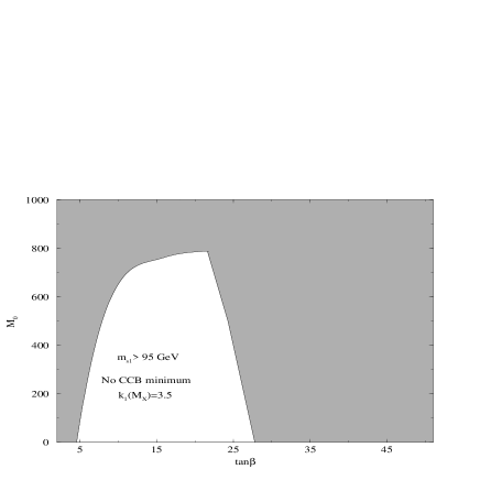
Figure 6: Taking $M_{2}=90$ GeV, we have plotted the parameter space which gives rise to charge and color conserving minima (unshaded region) in the $M_{0}-\tan\beta$ plane. When all the Yukawa couplings are at the fixed point $\tan\beta$ is typically $m_{t}/m_{b}\sim 40-60$. Note that there is no charge and color conserving solutions in this case. In this figure we have taken $k^{2}_{1}(M_{X})=4\pi$.

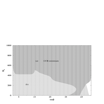
Figure 7: Taking $M_{2}=90$ GeV, we have plotted the parameter space which gives rise to charge and color conserving minima (unshaded region) in the $M_{0}-\tan\beta$ plane. Note that most of the plane is excluded. Region (b) is due to the effect of a vector-like slepton where as (a) is due to three light generations only. In this figure we have taken $k_{1}(M_{X})=0.1$.

$$\begin{array}[]{|c|c| c| c||c| c| c|}\hline\cr&\vrule\lx@intercol\hfil k_{1}(M_{X})=3.5\hfil\lx@intercol\vrule\lx@intercol\vrule\lx@intercol&\vrule\lx@intercol\hfil k_{1}(M_{X})=0.1\hfil\lx@intercol\vrule\lx@intercol\\ \hline\cr m_{i}(GeV)&\tan\beta=5&\tan\beta=30&\tan\beta=50&\tan\beta=5&\tan\beta=30&\tan\beta=50\\ \hline\cr m_{S_{1}}&120&105&107&115&119&116\\ m_{S_{2}},\,m_{S_{3}}&1061\,,1423&1227,\,1490&961,\,1171&1342,\,3950&1176,\,2124&847,\,1439\\ m_{a_{1}},\,m_{a_{2}}&1090,\,934&1219,\,1461&959,\,1455&1342,\,6840&1176,\,3678&847,\,2493\\ m_{H^{\pm}}&1061&1190&799&1344&1147&698\\ \hline\cr\end{array}$$

Table 4: Higgs masses after including one-loop radiative corrections to the scalar potential. $M_{Q}=3$ TeV ($M_{0}=0$), $M_{2}=90$ GeV (experimental lower bound on the wino mass).

3.5 EWSB without Charge and Color breaking

Stronger constraint on the parameter space at the unification scale are obtained demanding that no charge and color breaking (CCB) minima of the scalar potential is present at low energy[16]. Note that we cannot have charge and color breaking minima whereas we would like to have radiative EWSB and thereby a correct $m_{Z}$. Large Yukawa couplings drive the soft supersymmetry breaking mass terms to negative values provided the superparticles whose masses are being considered interacts via the large Yukawa coupling under consideration. For example a large top Yukawa coupling drives the Higgs masses to negative values triggering radiative electroweak breaking. From(4) we see that ESSM has a number of Yukawa couplings at the unification scale which couples to the colored superpartners. Hence there is a possibility that their large renormalization effects may lead to masses of superparticles with weak isospin and color quantum numbers which lead to charge and color breaking. This will be the situation when $M_{0}$ and/or $\tan\beta$ are large. Note that large $\tan\beta$ region has a large bottom quark coupling. To get the constraint in the plane $M_{0}$-$\tan\beta$ we verify that for each set of parameters corresponding to a correct EWSB minimum there is no deeper charge or color breaking minimum. The allowed parameter space obtained when $k_{1}(M_{X})=\sqrt{4\pi}$ is given in figure 6. We have also included the constraint $m_{S1}>95$ GeV which forbids low values of $\tan\beta$ whereas the CCB constraint excludes large values of $\tan\beta$. The constraint on the low values of $\tan\beta$ can be evaded if we reduce $k_{1}(M_{X})$(figure 7) .

Reducing $k_{1}$ implies allowing larger values of the couplings $z_{f}$ and $z^{\prime}_{c}$. This turns out to be enough to affect the masses of the extra generation sleptons which are the eigenvalues of the mass matrix

$${\cal M}^{2}(E^{\prime}_{L},E^{\prime}_{R})=\left(\matrix{\tilde{m}^{2}_{E_{L}}+z_{E}^{2}v_{\lambda}^{2}&z_{E}(k_{1}v_{1}v_{2}-k_{2}v_{\lambda}^{2}+A_{N}v_{\lambda})\cr z_{N}(k_{1}v_{1}v_{2}-k_{2}v_{\lambda}^{2}+A_{E}v_{\lambda}&\tilde{m}^{2}_{E_{R}}+z_{E}^{2}v_{\lambda}^{2}\cr}\right)\,,$$ (23)

where $\tilde{m}^{2}_{E_{i}}$ are the running mass parameters. Let us discuss the slepton masses for the time being in the context of electric charge breaking. Color breaking can be understood very similarly. For a vector-like scale of $M_{L}\sim M_{Q}/3\sim 1$ TeV the off-diagonal terms in the above mass matrix can compete with the diagonal ones. This increases the splitting between the eigenvalues and even rendering one of the eigenvalues negative. Coming back to RGE, this would be the situation for most of the parameter space when $k_{1}(M_{X})=0.1$ as shown in figure 7. Squared mass parameter of a neutral slepton becoming negative may only indicate that it would also get a VEV, and it may affect the values of the other VEVs. But a negative charged slepton squared mass parameter would imply a new source of electric charge breaking minima in ESSM. This should be understood parallel to EWSB. Note that a negative squared mass parameter of the doublet Higgs may not be enough to generate a EWSB minimum.

Thus in the small $k_{1}$ case save the parameter space lost due to CCB a small region corresponding to large values of $\tan\beta$ is all that remains. We point out that there is no such constraint due to the vector-like spectrum for larger values of $k_{1}$.

4 Conclusion

We question the commonly accepted notion of a unified gauge coupling $\alpha_{X}\sim 0.04$. If the Minimal Supersymmetric Standard Model (MSSM) is extended by including two vector-like families (ESSM) the couplings grow stronger than the low energy ones due to the renormalization effects of the extra matter and unify at a semi-perturbative scale of around $0.2$. This is actually the only extension of MSSM containing complete families of quarks and leptons that is permitted by measurements of the oblique electroweak parameters on one hand and renormalization group analysis on the other. The former restricts one to add only vector-like families whereas the latter states that no more than one pair of families can be added to maintain the perturbative unitarity up to the unification scale. In ESSM the weak SU(2) coupling grows by a factor of six at the unification scale compared to the weak-scale value (figure 1.a). The four dimensional string coupling may have a similar intermediate value which is large enough to make the dilaton stable as was conjectured by the previous authors[1]. ESSM has a unique pattern of the Yukawa matrices which is motivated by preon theories. The vector-like matter and normal matter has off diagonal Yukawa couplings whereas the normal three generations do not have Yukawa couplings among them at all. This leads to a see-saw like picture of the fermion masses. Below the mass scale of the vector-like generation a hierarchical mass pattern of chiral fermions emerge. If we fix all the Yukawa couplings to be large at the unification scale we get unique predictions of the low energy fermion masses when the Yukawa couplings approach their “quasi-infrared fixed points” at the scale of the top quark mass. On the contrary the renormalization effects of these relatively large Yukawa couplings have non-trivial effects on the unification of gauge couplings. Keeping this in mind we have also performed the renormalization group evolution of the gauge couplings taking into account the Yukawa effects at the two-loops. If we assume the universality of the soft supersymmetry-breaking parameters at the unification scale renormalization group evolution enable us to determine the supersymmetry spectrum at low energy quite easily. Note that due to the presence of the heavy generations the renormalization of the superparticle mass parameters are considerably different from that of MSSM as we would expect. This makes ESSM distinct from MSSM from the point of view of collider searches. The first and second generation squarks do not have large Yukawa renormalization hence they experience pronounced QCD renormalization which make them heavy (figure 3.b).

A further question will be to get the correct radiative electroweak breaking. We point out that the mass of the vector-like generations is actually linked to the electroweak symmetry breaking mechanism by the approximate relation $M_{Q}\sim(z_{q}/k_{1})\mu$. An electroweak symmetry breaking minimum which fits the mass of the Z boson exactly cannot be obtained in the “quasi-infrared fixed-point” scenario of the Yukawa couplings if we like $M_{Q}$ to be below $100$ TeVs. This is too large to be interesting experimentally. Thus at least some of the Yukawa couplings must have smaller values. The fixed-point scenario naturally have a large $\tan\beta$. We show that large $\tan\beta$ region suffers from the presence of Charge and Color breaking minima for any value of the vector-like scale from $m_{Z}$ up to $M_{X}$. So also in this case we find that to get a global charge and color conserving minima we must give up the assumption of all Yukawa couplings at their “quasi-infrared fixed point” in the case of ESSM.

5 Appendix

5.1 RGE coefficients of Yukawa couplings

The RGE for the Yukawa couplings (at any order) are given by the following general expression which is perturbatively exact

$$16\pi^{2}\frac{d\mbox{$h_{ij}^{m}$}}{dt}=\mbox{$h_{ik}^{m}$}(\gamma_{L})^{k}_{j}+(\gamma_{R})^{i}_{k}\mbox{$h_{kj}^{m}$}+\mbox{$h_{ij}^{m}$}\gamma_{H_{m}}\,.$$ (24)

In (24) $h_{ij}^{m}$ is the Yukawa coupling for the right-handed field $R_{i}$, the left-handed field $L_{j}$ and the scalar $H_{m}$. The functions $\gamma_{A}$ are the anomalous dimensions for the superfield $A$[20]. We define $h_{ij}^{m}$ as the Yukawa coupling matrix when all the superfields enter in the vertex and $h_{ij}^{m^{\dagger}}$ when they leave.

We have used the two-loop anomalous dimensions to evaluate the expression (24) which can be splitted as follows

$$(\gamma_{A})^{i}_{j}=(\gamma_{A}^{1})^{i}_{j}+\frac{1}{16\pi^{2}}(\gamma^{2}_{A})^{i}_{j}.$$ (25)

The component one-loop and two-loop parts are given by the expressions

$$(\gamma^{1}_{A})^{i}_{j} = \mbox{$h_{ik}^{m}$}\mbox{$h_{kj}^{m^{\dagger}}$}-2g_{a}^{2}C_{2}(R_{a})\delta_{ij}\,,$$ (26)

$$(\gamma^{2}_{A})^{i}_{j} = -\left(\mbox{$h_{ik}^{m}$}(\gamma^{(1)}_{B})^{k}_{l}\mbox{$h_{lj}^{m^{\dagger}}$}+\mbox{$h_{ik}^{m}$}\gamma^{(1)}_{H_{m}}\mbox{$h_{kj}^{m^{\dagger}}$}\right)+2b_{a}C_{2}(R_{a})g_{a}^{4}\delta_{ij}-2(\gamma_{A}^{(1)})^{i}_{j}C_{2}(R_{a})g_{a}^{2}\,.$$ (27)

We have denoted $g_{a}$ as the gauge coupling $b_{a}$ as in the one-loop gauge $\beta$-function and $C_{2}(R_{a})$ as the quadratic Casimir operator for the $R_{a}$ dimensional irreducible representation. The anomalous dimensions can be expanded in terms of four Yukawa coupling matrices $h^{m}_{f}$ related to equal number of Higgs bosons (at the unification scale they can be thought of a 10 and two singlets of SO(10)). The index $m$ assumes the values $m=H_{1},\,H_{2},\,H_{S},\,H_{\lambda}$ whereas $f=u,\,d,\,l,\,\nu$. The up sector Yukawa matrix can be re-expanded in terms of the individual matrices which are

x′q00000),fragments fragmentsx′𝑞00000\displaystyle\left(\begin{tabular}[]{ccc}0&$x_{u}$&0\\ $x^{\prime}_{q}$&0&0\\ 0&0&0\end{tabular}\right)\,,

$$h_{u}^{H_{2}} = \left(\begin{tabular}[]{ccc}0&$x_{u}$&0\\ $x^{\prime}_{q}$&0&0\\ 0&0&0\end{tabular}\right)\,,$$ 0xu00xu0 (31)

$$h_{u}^{H_{S}} = \left(\begin{tabular}[]{ccc}0&0&$y_{u}$\\ 0&0&0\\ $y^{\prime}_{q}/\sqrt{2}$&0&0\end{tabular}\right)\,,$$ (35)

$$h_{u}^{H_{\lambda}} = \left(\begin{tabular}[]{ccc}0&0&0\\ 0&0&$z_{u}$\\ 0&$z^{\prime}_{q}/\sqrt{2}$&0\end{tabular}\right)\,.$$ (39)

We will have similar expressions for the down-quark sector and similarly for the leptonic sector. The normalization factor $\sqrt{2}$ avoids over counting when we sum over the index $f=u,\,d$ or $f=l,\,\nu$.

The one-loop anomalous dimensions for the quark sector are as follows

$$(\mbox{$\gamma_{\bar{u}}^{1}$})_{ij} = 2(\mbox{$h_{u}^{H_{2}}$}\mbox{$h_{u}^{{H_{2}}^{\dagger}}$})_{ij}+(\mbox{$h_{u}^{H_{S}}$}\mbox{$h_{u}^{{H_{S}}^{\dagger}}$})_{ij}+(\mbox{$h_{u}^{H_{\lambda}}$}\mbox{$h_{u}^{{H_{\lambda}}^{\dagger}}$})_{ij}-\left(\frac{8}{15}g_{1}^{2}+\frac{8}{3}g_{3}^{2}\right)\delta_{ij}\,,$$ (40)

$$(\mbox{$\gamma_{\bar{d}}^{1}$})_{ij} = 2(\mbox{$h_{d}^{H_{1}}$}\mbox{$h_{d}^{{H_{1}}^{\dagger}}$})_{ij}+(\mbox{$h_{d}^{H_{S}}$}\mbox{$h_{d}^{{H_{S}}^{\dagger}}$})_{ij}+(\mbox{$h_{d}^{H_{\lambda}}$}\mbox{$h_{d}^{{H_{\lambda}}^{\dagger}}$})_{ij}-(\frac{2}{15}g_{1}^{2}+\frac{8}{3}g_{3}^{2})\delta_{ij}\,,$$ (41)

$$(\mbox{$\gamma_{q}^{1}$})_{ij} = (\mbox{$h_{u}^{{H_{2}}^{\dagger}}$}\mbox{$h_{u}^{H_{2}}$})_{ij}+(\mbox{$h_{d}^{{H_{1}}^{\dagger}}$}\mbox{$h_{d}^{H_{1}}$})_{ij}+(\mbox{$h_{u}^{{H_{S}}^{\dagger}}$}\mbox{$h_{u}^{H_{S}}$})_{ij}+(\mbox{$h_{d}^{{H_{S}}^{\dagger}}$}\mbox{$h_{d}^{H_{S}}$})_{ij}+(\mbox{$h_{u}^{{H_{\lambda}}^{\dagger}}$}\mbox{$h_{u}^{H_{\lambda}}$})_{ij}$$

$$+(\mbox{$h_{d}^{{H_{\lambda}}^{\dagger}}$}\mbox{$h_{d}^{H_{\lambda}}$})_{ij}-(\frac{1}{30}g_{1}^{2}+\frac{3}{2}g_{2}^{2}+\frac{8}{3}g_{3}^{2})\delta_{ij}\,,$$

$$\;\;\;\;\;\;\;\;i,j=1,2\;$$

$$\gamma_{U}^{1} = (\mbox{$h_{u}^{{H_{\lambda}}^{\dagger}}$}\mbox{$h_{u}^{H_{\lambda}}$})_{(3,3)}+(\mbox{$h_{u}^{{H_{S}}^{\dagger}}$}\mbox{$h_{u}^{H_{S}}$})_{(3,3)}-\frac{8}{15}g_{1}^{2}-\frac{8}{3}g_{3}^{2}\,,$$ (43)

$$\gamma_{D}^{1} = (\mbox{$h_{d}^{{H_{\lambda}}^{\dagger}}$}\mbox{$h_{d}^{H_{\lambda}}$})_{(3,3)}+(\mbox{$h_{d}^{{H_{S}}^{\dagger}}$}\mbox{$h_{d}^{H_{S}}$})_{(3,3)}-\frac{2}{15}g_{1}^{2}-\frac{8}{3}g_{3}^{2}\,,$$

$$\gamma_{\bar{Q}}^{1} = (\mbox{$h_{u}^{H_{\lambda}}$}\mbox{$h_{u}^{{H_{\lambda}}^{\dagger}}$})_{(3,3)}+(\mbox{$h_{d}^{H_{\lambda}}$}\mbox{$h_{d}^{{H_{\lambda}}^{\dagger}}$})_{(3,3)}+(\mbox{$h_{u}^{H_{S}}$}\mbox{$h_{u}^{{H_{S}}^{\dagger}}$})_{(3,3)}+(\mbox{$h_{d}^{H_{S}}$}\mbox{$h_{d}^{{H_{S}}^{\dagger}}$})_{(3,3)}$$

$$-\frac{1}{30}g_{1}^{2}-\frac{3}{2}g_{2}^{2}-\frac{8}{3}g_{3}^{2}\,,$$

$$\gamma_{\bar{U}}^{1} = \left(\begin{tabular}[]{cc}$(\mbox{$\gamma_{\bar{u}}^{1}$})_{ij}$&0\\ 0&$\mbox{$\gamma_{\bar{Q}}^{1}$}$\end{tabular}\right)\,,$$ (48)

$$\gamma_{\bar{D}}^{1} = \left(\begin{tabular}[]{cc}$(\mbox{$\gamma_{\bar{d}}^{1}$})_{ij}$&0\\ 0&$\mbox{$\gamma_{\bar{Q}}^{1}$}$\end{tabular}\right)\,,$$ (51)

$$\gamma_{Q_{u}}^{1} = \left(\begin{tabular}[]{cc}$(\mbox{$\gamma_{q}^{1}$})_{ij}$&0\\ 0&\mbox{$\gamma_{U}^{1}$}\end{tabular}\right)\,,$$ (54)

$$\gamma_{Q_{d}}^{1} = \left(\begin{tabular}[]{cc}$(\mbox{$\gamma_{q}^{1}$})_{ij}$&0\\ 0&\mbox{$\gamma_{D}^{1}$}\end{tabular}\right)\,.$$ (57)

The two-loop contributions to the anomalous dimensions for the quark sector are as follows

$$(\mbox{$\gamma_{\bar{u}}^{2}$})_{ij} = -\left(2\mbox{$h_{u}^{H_{2}}$}(\mbox{$\gamma_{Q_{u}}^{1}$}+\mbox{$\gamma_{H_{2}}^{1}$})\mbox{$h_{u}^{{H_{2}}^{\dagger}}$}+\mbox{$h_{u}^{H_{S}}$}(\mbox{$\gamma_{Q_{u}}^{1}$}+\mbox{$\gamma_{H_{S}}^{1}$})\mbox{$h_{u}^{{H_{S}}^{\dagger}}$}+\mbox{$h_{u}^{H_{\lambda}}$}(\mbox{$\gamma_{Q_{u}}^{1}$}+\mbox{$\gamma_{H_{\lambda}}^{1}$})\mbox{$h_{u}^{{H_{\lambda}}^{\dagger}}$}\right)_{ij}$$ (58)

$$-\left(\frac{8}{15}g_{1}^{2}+\frac{8}{3}g_{3}^{2}\right)(\mbox{$\gamma_{\bar{u}}^{1}$})_{ij}+\left(\frac{8}{15}b_{1}g_{1}^{4}+\frac{8}{3}b_{3}g_{3}^{4}\right)\delta_{ij}$$

$$(\mbox{$\gamma_{\bar{d}}^{2}$})_{ij} = -\left(2\mbox{$h_{d}^{H_{1}}$}(\mbox{$\gamma_{Q_{d}}^{1}$}+\mbox{$\gamma_{H_{1}}^{1}$})\mbox{$h_{d}^{{H_{1}}^{\dagger}}$}+\mbox{$h_{d}^{H_{S}}$}(\mbox{$\gamma_{Q_{d}}^{1}$}+\mbox{$\gamma_{H_{S}}^{1}$})\mbox{$h_{d}^{{H_{S}}^{\dagger}}$}+\mbox{$h_{d}^{H_{\lambda}}$}(\mbox{$\gamma_{Q_{d}}^{1}$}+\mbox{$\gamma_{H_{\lambda}}^{1}$})\mbox{$h_{d}^{{H_{\lambda}}^{\dagger}}$}\right)_{ij}$$ (59)

$$-\left(\frac{2}{15}g_{1}^{2}+\frac{8}{3}g_{3}^{2}\right)(\mbox{$\gamma_{\bar{d}}^{1}$})_{ij}+\left(\frac{2}{15}b_{1}g_{1}^{4}+\frac{8}{3}b_{3}g_{3}^{4}\right)\delta_{ij}\,,$$

$$(\mbox{$\gamma_{q}^{2}$})_{ij} = (\mbox{$h_{u}^{{H_{2}}^{\dagger}}$}(\mbox{$\gamma_{\bar{U}}^{1}$}+\mbox{$\gamma_{H_{2}}^{1}$})\mbox{$h_{u}^{H_{2}}$}+\mbox{$h_{d}^{{H_{1}}^{\dagger}}$}(\mbox{$\gamma_{\bar{D}}^{1}$}+\mbox{$\gamma_{H_{1}}^{1}$})\mbox{$h_{d}^{H_{1}}$}+\mbox{$h_{u}^{{H_{S}}^{\dagger}}$}(\mbox{$\gamma_{\bar{U}}^{1}$}+\mbox{$\gamma_{H_{S}}^{1}$})\mbox{$h_{u}^{H_{S}}$}+\mbox{$h_{d}^{{H_{S}}^{\dagger}}$}(\mbox{$\gamma_{\bar{D}}^{1}$}+\mbox{$\gamma_{H_{S}}^{1}$})\mbox{$h_{d}^{H_{S}}$}$$ (60)

$$+\mbox{$h_{u}^{{H_{\lambda}}^{\dagger}}$}(\mbox{$\gamma_{\bar{U}}^{1}$}+\mbox{$\gamma_{H_{\lambda}}^{1}$})\mbox{$h_{u}^{H_{\lambda}}$}+\mbox{$h_{d}^{{H_{\lambda}}^{\dagger}}$}(\mbox{$\gamma_{\bar{D}}^{1}$}+\mbox{$\gamma_{H_{\lambda}}^{1}$})\mbox{$h_{d}^{H_{\lambda}}$})_{ij}$$

$$-\left(\frac{1}{30}g_{1}^{2}+\frac{3}{2}g_{2}^{2}+\frac{8}{3}g_{3}^{2}\right)(\mbox{$\gamma_{q}^{1}$})_{ij}+\left(\frac{1}{30}b_{1}g_{1}^{4}+\frac{3}{2}b_{2}g_{2}^{4}+\frac{8}{3}b_{3}g_{3}^{4}\right)\delta_{ij}\,,$$

$$\gamma_{U}^{2} = -\left(\mbox{$h_{u}^{{H_{\lambda}}^{\dagger}}$}(\mbox{$\gamma_{\bar{U}}^{1}$}+\mbox{$\gamma_{H_{\lambda}}^{1}$})\mbox{$h_{u}^{H_{\lambda}}$}+\mbox{$h_{u}^{{H_{S}}^{\dagger}}$}(\mbox{$\gamma_{\bar{U}}^{1}$}+\mbox{$\gamma_{H_{S}}^{1}$})\mbox{$h_{u}^{H_{S}}$}\right)_{(3,3)}$$ (61)

$$-\left(\frac{8}{15}g_{1}^{2}+\frac{8}{3}g_{3}^{2}\right)\mbox{$\gamma_{U}^{1}$}+\frac{8}{15}b_{1}g_{1}^{4}+\frac{8}{3}b_{3}g_{3}^{4}\,,$$

$$\gamma_{D}^{2} = -\left(\mbox{$h_{d}^{{H_{\lambda}}^{\dagger}}$}(\mbox{$\gamma_{\bar{D}}^{1}$}+\mbox{$\gamma_{H_{\lambda}}^{1}$})\mbox{$h_{d}^{H_{\lambda}}$}+\mbox{$h_{d}^{{H_{S}}^{\dagger}}$}(\mbox{$\gamma_{\bar{D}}^{1}$}+\mbox{$\gamma_{H_{S}}^{1}$})\mbox{$h_{d}^{H_{S}}$}\right)_{(3,3)}$$ (62)

$$-\left(\frac{2}{15}g_{1}^{2}+\frac{8}{3}g_{3}^{2}\right)\mbox{$\gamma_{D}^{1}$}+\frac{2}{15}b_{1}g_{1}^{4}+\frac{8}{3}b_{3}g_{3}^{4}\,,$$

$$\gamma_{\bar{Q}}^{2} = -\left(\mbox{$h_{u}^{H_{\lambda}}$}(\mbox{$\gamma_{Q_{u}}^{1}$}+\mbox{$\gamma_{H_{\lambda}}^{1}$})\mbox{$h_{u}^{{H_{\lambda}}^{\dagger}}$}+\mbox{$h_{d}^{H_{\lambda}}$}(\mbox{$\gamma_{Q_{d}}^{1}$}+\mbox{$\gamma_{H_{\lambda}}^{1}$})\mbox{$h_{d}^{{H_{\lambda}}^{\dagger}}$}+\mbox{$h_{u}^{H_{S}}$}(\mbox{$\gamma_{Q_{u}}^{1}$}+\mbox{$\gamma_{H_{S}}^{1}$})\mbox{$h_{u}^{{H_{S}}^{\dagger}}$}+\mbox{$h_{d}^{H_{S}}$}(\mbox{$\gamma_{Q_{d}}^{1}$}+\mbox{$\gamma_{H_{S}}^{1}$})\mbox{$h_{d}^{{H_{S}}^{\dagger}}$}\right)_{(3,3)}$$ (63)

$$-\left(\frac{1}{30}g_{1}^{2}+\frac{3}{2}g_{2}^{2}+\frac{8}{3}g_{3}^{2}\right)\mbox{$\gamma_{\bar{Q}}^{1}$}+\frac{1}{30}b_{1}g_{1}^{4}+\frac{3}{2}b_{2}g_{2}^{4}+\frac{8}{3}b_{3}g_{3}^{4}.$$

Two-loop anomalous dimensions of leptons can be obtained from the above expressions with the replacements $u\rightarrow\nu$, $d\rightarrow e$ and $q\rightarrow l$.

We have set the Yukawa couplings for the first and second generation to zero. They can be included by the replacement of the numbers $x_{f}$, $x^{\prime}_{c}$, $y_{f}$ and $y^{\prime}_{c}$ by corresponding three dimensional vectors. In this case $3\times 3$ Yukawa matrices given in equations (31-39) will become $5\times 5$ matrices.

The one-loop and two-loop anomalous dimensions for the Higgs scalars are as follows

(a) one-loop anomalous dimensions

$$\gamma_{H_{1}}^{1} = 3Tr[\mbox{$h_{d}^{H_{1}}$}\mbox{$h_{d}^{{H_{1}}^{\dagger}}$}]+Tr[\mbox{$h_{e}^{H_{1}}$}\mbox{$h_{e}^{{H_{1}}^{\dagger}}$}]+k_{1}^{2}-\frac{3}{10}g_{1}^{2}-\frac{3}{2}g_{2}^{2}\,,$$ (64)

$$\gamma_{H_{2}}^{1} = 3Tr[\mbox{$h_{u}^{H_{1}}$}\mbox{$h_{u}^{{H_{1}}^{\dagger}}$}]+Tr[\mbox{$h_{\nu}^{H_{1}}$}\mbox{$h_{\nu}^{{H_{1}}^{\dagger}}$}]+k_{1}^{2}-\frac{3}{10}g_{1}^{2}-\frac{3}{2}g_{2}^{2}\,,$$ (65)

$$\gamma_{H_{S}}^{1} = 6Tr[\mbox{$h_{d}^{H_{S}}$}\mbox{$h_{d}^{{H_{S}}^{\dagger}}$}+\mbox{$h_{u}^{H_{S}}$}\mbox{$h_{u}^{{H_{S}}^{\dagger}}$}]+2Tr[\mbox{$h_{e}^{H_{S}}$}\mbox{$h_{e}^{{H_{S}}^{\dagger}}$}+\mbox{$h_{\nu}^{H_{S}}$}\mbox{$h_{\nu}^{{H_{S}}^{\dagger}}$}]+k_{3}^{2}\,,$$ (66)

$$\gamma_{H_{\lambda}}^{1} = 6Tr[\mbox{$h_{d}^{H_{\lambda}}$}\mbox{$h_{d}^{{H_{\lambda}}^{\dagger}}$}+\mbox{$h_{u}^{H_{\lambda}}$}\mbox{$h_{u}^{{H_{\lambda}}^{\dagger}}$}]+2Tr[\mbox{$h_{e}^{H_{\lambda}}$}\mbox{$h_{e}^{{H_{\lambda}}^{\dagger}}$}+\mbox{$h_{\nu}^{H_{\lambda}}$}\mbox{$h_{\nu}^{{H_{\lambda}}^{\dagger}}$}]+2k_{1}^{2}+k_{2}^{2}.$$ (67)

(a) two-loop contributions to the anomalous dimensions

$$\gamma_{H_{1}}^{2} = -3Tr[\mbox{$h_{d}^{H_{1}}$}\mbox{$\gamma_{Q_{d}}^{1}$}\mbox{$h_{d}^{{H_{1}}^{\dagger}}$}+\mbox{$h_{d}^{{H_{1}}^{\dagger}}$}\mbox{$\gamma_{\bar{D}}^{1}$}\mbox{$h_{d}^{H_{1}}$}]-Tr[\mbox{$h_{e}^{H_{1}}$}\mbox{$\gamma_{L_{e}}^{1}$}\mbox{$h_{e}^{{H_{1}}^{\dagger}}$}+\mbox{$h_{e}^{{H_{1}}^{\dagger}}$}\mbox{$\gamma_{\bar{E}}^{1}$}\mbox{$h_{e}^{H_{1}}$}]$$ (68)

$$-k_{1}(\mbox{$\gamma_{H_{1}}^{1}$}+\mbox{$\gamma_{H_{\lambda}}^{1}$})k_{1}-\left(\frac{3}{10}g_{1}^{2}+\frac{3}{2}g_{2}^{2}\right)\mbox{$\gamma_{H_{1}}^{1}$}+\frac{3}{10}b_{1}g_{1}^{4}+\frac{3}{2}b_{2}g_{2}^{4}\,,$$

$$\gamma_{H_{2}}^{2} = -3Tr[\mbox{$h_{u}^{H_{1}}$}\mbox{$\gamma_{Q_{u}}^{1}$}\mbox{$h_{u}^{{H_{1}}^{\dagger}}$}+\mbox{$h_{u}^{{H_{1}}^{\dagger}}$}\mbox{$\gamma_{\bar{U}}^{1}$}\mbox{$h_{u}^{H_{1}}$}]-Tr[\mbox{$h_{\nu}^{H_{1}}$}\mbox{$\gamma_{L_{\nu}}^{1}$}\mbox{$h_{\nu}^{{H_{1}}^{\dagger}}$}+\mbox{$h_{\nu}^{{H_{1}}^{\dagger}}$}\mbox{$\gamma_{\bar{\nu}}^{1}$}\mbox{$h_{\nu}^{H_{1}}$}]$$ (69)

$$-k_{1}(\mbox{$\gamma_{H_{2}}^{1}$}+\mbox{$\gamma_{H_{\lambda}}^{1}$})k_{1}-\left(\frac{3}{10}g_{1}^{2}+\frac{3}{2}g_{2}^{2}\right)\mbox{$\gamma_{H_{2}}^{1}$}+\frac{3}{10}b_{1}g_{1}^{4}+\frac{3}{2}b_{2}g_{2}^{4}\,,$$

$$\gamma_{H_{S}}^{2} = -6Tr[\mbox{$h_{d}^{H_{S}}$}\mbox{$\gamma_{Q_{d}}^{1}$}\mbox{$h_{d}^{{H_{S}}^{\dagger}}$}+\mbox{$h_{d}^{{H_{S}}^{\dagger}}$}\mbox{$\gamma_{\bar{D}}^{1}$}\mbox{$h_{d}^{H_{S}}$}+\mbox{$h_{u}^{H_{S}}$}\mbox{$\gamma_{Q_{u}}^{1}$}\mbox{$h_{u}^{{H_{S}}^{\dagger}}$}+\mbox{$h_{u}^{{H_{S}}^{\dagger}}$}\mbox{$\gamma_{\bar{U}}^{1}$}\mbox{$h_{u}^{H_{S}}$}]$$

$$-2Tr[\mbox{$h_{e}^{H_{S}}$}\mbox{$\gamma_{L_{e}}^{1}$}\mbox{$h_{e}^{{H_{S}}^{\dagger}}$}+\mbox{$h_{e}^{{H_{S}}^{\dagger}}$}\mbox{$\gamma_{\bar{E}}^{1}$}\mbox{$h_{e}^{H_{S}}$}+\mbox{$h_{\nu}^{H_{S}}$}\mbox{$\gamma_{L_{\nu}}^{1}$}\mbox{$h_{\nu}^{{H_{S}}^{\dagger}}$}+\mbox{$h_{\nu}^{{H_{S}}^{\dagger}}$}\mbox{$\gamma_{\bar{\nu}}^{1}$}\mbox{$h_{\nu}^{H_{S}}$}]$$

$$-k_{3}\mbox{$\gamma_{H_{S}}^{1}$}k_{3},$$

$$\gamma_{H_{\lambda}}^{2} = -6Tr[\mbox{$h_{d}^{H_{\lambda}}$}\mbox{$\gamma_{Q_{d}}^{1}$}\mbox{$h_{d}^{{H_{\lambda}}^{\dagger}}$}+\mbox{$h_{d}^{{H_{\lambda}}^{\dagger}}$}\mbox{$\gamma_{\bar{D}}^{1}$}\mbox{$h_{d}^{H_{\lambda}}$}+\mbox{$h_{u}^{H_{\lambda}}$}\mbox{$\gamma_{Q_{u}}^{1}$}\mbox{$h_{u}^{{H_{\lambda}}^{\dagger}}$}+\mbox{$h_{u}^{{H_{\lambda}}^{\dagger}}$}\mbox{$\gamma_{\bar{U}}^{1}$}\mbox{$h_{u}^{H_{\lambda}}$}]$$ (70)

$$-2Tr[\mbox{$h_{e}^{H_{\lambda}}$}\mbox{$\gamma_{L_{e}}^{1}$}\mbox{$h_{e}^{{H_{\lambda}}^{\dagger}}$}+\mbox{$h_{e}^{{H_{\lambda}}^{\dagger}}$}\mbox{$\gamma_{\bar{E}}^{1}$}\mbox{$h_{e}^{H_{\lambda}}$}+\mbox{$h_{\nu}^{H_{\lambda}}$}\mbox{$\gamma_{L_{\nu}}^{1}$}\mbox{$h_{\nu}^{{H_{\lambda}}^{\dagger}}$}+\mbox{$h_{\nu}^{{H_{\lambda}}^{\dagger}}$}\mbox{$\gamma_{\bar{\nu}}^{1}$}\mbox{$h_{\nu}^{H_{\lambda}}$}]$$

$$-k_{3}\mbox{$\gamma_{H_{\lambda}}^{1}$}k_{3}.$$

5.2 Two-loop formulae of threshold corrections in step-function approximation.

The two-loop coefficient for the RGE of the gauge coupling $b_{ij}$ and $a_{i}^{(k)}$ including the threshold corrections are listed here. $\theta_{i}$ is the step function. The mass thresholds are denoted by the index $i=\tilde{w},\tilde{g},\tilde{q}_{L},\,\tilde{u}_{R},\,\tilde{d}_{R},\,\tilde{l}_{L},\,\tilde{e}_{R},\,\tilde{h},\,H$ and similarly the vector-like thresholds $i=Q,\,L$. Here $n_{f}$ is the number of chiral generations and $n_{V}$ is the number of extra generations.

(a) Gauge contribution

$$b_{11} = n_{f}\left(\frac{19}{15}+\left(2-\mbox{$\theta_{\tilde{w}}$}\right)\left(\frac{9}{100}\mbox{$\theta_{\tilde{l}_{L}}$}+\frac{18}{25}\mbox{$\theta_{\tilde{e}_{R}}$}+\frac{2}{75}\mbox{$\theta_{\tilde{d}_{R}}$}+\frac{1}{300}\mbox{$\theta_{\tilde{q}_{L}}$}+\frac{32}{75}\mbox{$\theta_{\tilde{u}_{R}}$}\right)\right)$$ (71)

$$+\frac{9}{50}\left(1+\mbox{$\theta_{H}$}+\mbox{$\theta_{\tilde{h}}$}\left(1-\mbox{$\theta_{\tilde{w}}$}\right)\right)$$

$$+n_{V}\left(3-\mbox{$\theta_{\tilde{w}}$}\right)\left(\frac{81}{100}\mbox{$\theta_{L}$}+\frac{137}{300}\mbox{$\theta_{Q}$}\right)\,,$$

$$b_{12} = n_{f}\left(\frac{3}{5}+\left(2-\mbox{$\theta_{\tilde{w}}$}\right)\left(\frac{9}{20}\mbox{$\theta_{\tilde{l}_{L}}$}+\frac{3}{20}\mbox{$\theta_{\tilde{q}_{L}}$}\right)\right)$$ (72)

$$+\frac{9}{10}\left(1+\mbox{$\theta_{H}$}+\mbox{$\theta_{\tilde{h}}$}\left(1-\mbox{$\theta_{\tilde{w}}$}\right)\right)$$

$$+n_{V}\left(3-\mbox{$\theta_{\tilde{w}}$}\right)\left(\frac{9}{20}\mbox{$\theta_{L}$}+\frac{3}{20}\mbox{$\theta_{Q}$}\right)\,,$$

$$b_{13} = n_{f}\left(\frac{44}{15}+\left(2-\mbox{$\theta_{\tilde{g}}$}\right)\left(\frac{4}{15}\mbox{$\theta_{\tilde{q}_{L}}$}+\frac{6}{15}\mbox{$\theta_{\tilde{d}_{R}}$}+\frac{32}{15}\mbox{$\theta_{\tilde{u}_{R}}$}\right)\right)$$ (73)

$$+n_{V}\left(3-\mbox{$\theta_{\tilde{g}}$}\right)\frac{44}{15}\mbox{$\theta_{Q}$}\,,$$

$$b_{21} = n_{f}\left(\frac{1}{5}+\left(2-\mbox{$\theta_{\tilde{w}}$}\right)\left(\frac{3}{20}\mbox{$\theta_{\tilde{l}_{L}}$}+\frac{1}{20}\mbox{$\theta_{\tilde{q}_{L}}$}\right)\right)$$ (74)

$$+\frac{3}{10}\left(1+\mbox{$\theta_{H}$}+\mbox{$\theta_{\tilde{h}}$}\left(1-\mbox{$\theta_{\tilde{w}}$}\right)\right)$$

$$+n_{V}\left(3-\mbox{$\theta_{\tilde{w}}$}\right)\left(\frac{3}{20}\mbox{$\theta_{L}$}+\frac{1}{20}\mbox{$\theta_{Q}$}\right)\,,$$

$$b_{22} = -\frac{136}{3}+\frac{64}{3}\mbox{$\theta_{\tilde{w}}$}+n_{f}\left(\frac{49}{3}+\left(26-33\mbox{$\theta_{\tilde{w}}$}\right)\left(\frac{1}{12}\mbox{$\theta_{\tilde{l}_{L}}$}+\frac{1}{4}\mbox{$\theta_{\tilde{q}_{L}}$}\right)\right)$$ (75)

$$+\left(\frac{13}{6}+\frac{13}{6}\mbox{$\theta_{H}$}+\mbox{$\theta_{\tilde{h}}$}\left(\frac{49}{6}-\frac{11}{2}\mbox{$\theta_{\tilde{w}}$}\right)\right)$$

$$+n_{V}\left(25-11\mbox{$\theta_{\tilde{w}}$}\right)\left(\frac{1}{4}\mbox{$\theta_{L}$}+\frac{3}{4}\mbox{$\theta_{Q}$}\right)\,,$$

$$b_{23} = n_{f}\left(4+4\left(2-\mbox{$\theta_{\tilde{g}}$}\right)\mbox{$\theta_{\tilde{q}_{L}}$}\right)$$ (76)

$$+n_{V}4\left(3-\mbox{$\theta_{\tilde{g}}$}\right)\mbox{$\theta_{Q}$}\,,$$

$$b_{31} = n_{f}\left(\frac{11}{30}+\left(2-\mbox{$\theta_{\tilde{g}}$}\right)\left(\frac{1}{30}\mbox{$\theta_{\tilde{q}_{L}}$}+\frac{1}{15}\mbox{$\theta_{\tilde{d}_{R}}$}+\frac{4}{15}\mbox{$\theta_{\tilde{u}_{R}}$}\right)\right)$$ (77)

$$+n_{V}\frac{11}{30}\left(3-\mbox{$\theta_{\tilde{g}}$}\right)\mbox{$\theta_{Q}$}\,,$$

$$b_{32} = n_{f}\left(\frac{3}{2}+\frac{3}{2}\left(2-\mbox{$\theta_{\tilde{g}}$}\right)\mbox{$\theta_{\tilde{q}_{L}}$}\right)$$ (78)

$$+n_{V}\frac{3}{2}\left(3-\mbox{$\theta_{\tilde{g}}$}\right)\mbox{$\theta_{Q}$}\,,$$

$$b_{33} = -102+48\mbox{$\theta_{\tilde{g}}$}+n_{f}\left(\frac{76}{3}+\left(\frac{11}{3}-\frac{13}{3}\mbox{$\theta_{\tilde{g}}$}\right)\left(2\mbox{$\theta_{\tilde{q}_{L}}$}+\mbox{$\theta_{\tilde{d}_{R}}$}+\mbox{$\theta_{\tilde{u}_{R}}$}\right)\right)$$ (79)

$$+n_{V}\left(40-\frac{52}{3}\mbox{$\theta_{\tilde{g}}$}\right)\mbox{$\theta_{Q}$}.$$

(b) Now the coefficients $a_{i}^{k}$: Let us become careful here. We define $\hat{\gamma}_{j}^{1}$ to be the anomalous dimensions without the gauge contributions which are as follows

$$\sum_{k}a_{1}^{k} = \frac{6}{5}\left(\frac{4}{3}\left(Tr\mbox{$\hat{\gamma}_{\bar{u}}^{1}$}+\mbox{$\hat{\gamma}_{U}^{1}$}\right)+\frac{1}{3}\left(Tr\mbox{$\hat{\gamma}_{\bar{d}}^{1}$}+\mbox{$\hat{\gamma}_{D}^{1}$}\right)+\frac{1}{6}\left(Tr\mbox{$\hat{\gamma}_{q}^{1}$}+\mbox{$\hat{\gamma}_{\bar{Q}}^{1}$}\right)+Tr\mbox{$\hat{\gamma}_{e}^{1}$}+\mbox{$\hat{\gamma}_{E}^{1}$}+\frac{1}{2}\left(Tr\mbox{$\hat{\gamma}_{l}^{1}$}+\mbox{$\hat{\gamma}_{L}^{1}$}\right)\right.$$ (80)

$$\left.+\frac{1}{2}\left(\mbox{$\hat{\gamma}_{H_{1}}^{1}$}+\mbox{$\hat{\gamma}_{H_{2}}^{1}$}\right)\right)\,,$$

$$\sum_{k}a_{2}^{k} = 3\left(Tr\mbox{$\hat{\gamma}_{q}^{1}$}+\mbox{$\hat{\gamma}_{\bar{Q}}^{1}$}\right)+Tr\mbox{$\hat{\gamma}_{l}^{1}$}+\mbox{$\hat{\gamma}_{\bar{L}}^{1}$}+\mbox{$\hat{\gamma}_{H_{1}}^{1}$}+\mbox{$\hat{\gamma}_{H_{2}}^{1}$}\,,$$ (81)

$$\sum_{k}a_{3}^{k} = Tr\mbox{$\hat{\gamma}_{\bar{u}}^{1}$}+Tr\mbox{$\hat{\gamma}_{\bar{d}}^{1}$}+\mbox{$\hat{\gamma}_{U}^{1}$}+\mbox{$\hat{\gamma}_{D}^{1}$}+2\left(Tr\mbox{$\hat{\gamma}_{q}^{1}$}+\mbox{$\hat{\gamma}_{\bar{Q}}^{1}$}\right)\,.$$ (82)

The vector-like superfields are massive at the scales ($M_{Q}$, $M_{L}$). After the rotation of the Yukawa matrices we get

$$\mbox{$h_{u}^{H_{2}}$}(\mu<M_{Q}) = \left(\begin{tabular}[]{ccc}$h_{t}(\mu)$&0&0\\ 0&0&0\\ 0&0&0\end{tabular}\right)\,,$$ (86)

$$\mbox{$h_{u}^{H_{S}}$}(\mu<M_{Q}) = \mbox{$h_{u}^{H_{\lambda}}$}(\mu<M_{Q})=0\,,$$ (87)

$$\mbox{$h_{d}^{H_{1}}$}(\mu<M_{Q}) = \left(\begin{tabular}[]{ccc}$h_{b}(\mu)$&0&0\\ 0&0&0\\ 0&0&0\end{tabular}\right)\,,$$ (91)

$$\mbox{$h_{d}^{H_{S}}$}(\mu<M_{Q}) = \mbox{$h_{d}^{H_{\lambda}}$}(\mu<M_{Q})=0\,,$$ (92)

$$\mbox{$h_{e}^{H_{1}}$}(\mu<M_{L}) = \left(\begin{tabular}[]{ccc}$h_{\tau}(\mu)$&0&0\\ 0&0&0\\ 0&0&0\end{tabular}\right)\,,$$ (96)

$$\mbox{$h_{e}^{H_{S}}$}(\mu<M_{L}) = \mbox{$h_{e}^{H_{\lambda}}$}(\mu<M_{L})=0\,,$$ (97)

with our boundary conditions(5).

References

• [1] K. S. Babu and J. C. Pati, Phys. Lett B384, (1996) 140.
• [2] P. Langacker and N. Polonsky, Phys. Rev. D52, (1995) 3081.
• [3] P. Ginsparg, Phys. Lett. B 197, (1987) 139; V. S. Kaplenovsky, Nucl. Phys. B 307, (1988) 145; erratum ibid. B442, (1995) 461.
• [4] K.S. Babu, K. Choi, J.C. Pati and X. Zhang, Phys. Lett. B333 (1994) 364.
• [5] M. Peskin and T. Takeuchi, Phys. Rev. Lett. 65, (1990) 964; G.Altarelli, R. Barbieri and S. Jadach, Nucl. Phys. B369, (1992) 3.
• [6] K. S. Babu, J. C. Pati and H. Stremnitzer, Phys. Rev. Lett 67, (1991) 1688; Phys. Rev. D51, (1995) 2451.
• [7] D. C. Kennedy and B. W. Lynn, Nucl. Phys. B322, (1989) 1; A. E. Faraggi and B. Grinstein, Nucl. Phys. B 422, (1994) 3; M. Bastero-Gil and J. Perez-Mercader, Nucl. Phys. B450, (1995) 21.
• [8] P. Chankowski, Z. Pluciennik and S. Pokorski, Nucl. Phys. B439, (1995)23; R. Barbieri, P. Ciafaloni and A. Strumia, Nucl. Phys. B442, (1995) 461; J. Bagger, K. Machev and D. Pierce, Phys. Lett. B 348, (1995) 443. M. Bastero-Gil and B. Brahmachari, Phys. Rev. D54, (1996) 1063; B. Brahmachari and R. N. Mohapatra, Phys. Lett. B 357, (1995), 566.
• [9] C. Kolda, J. March-Russell, Phys. Rev. D55, (1997) 4252.
• [10] L. Maiani, G. Parisi and R. Petronzio, Nucl. Phys. B136, (1978) 115; R. Hempfling, Phys. Lett B351, (1995) 206; B. Brahmachari, U. Sarkar and K. Sridhar, Mod. Phys. Lett A8, (1993) 3349; D. Ghilencea, M. Lanzagorta and G. G. Ross, Phys. Lett B415, (1997) 253; Nucl. Phys. B511, (1998) 3; G. Amelino-Camelia, D. ghilancea and G. G. Ross, Nucl. Phys. B528, (1998) 35.
• [11] K. Inoue et al, Prog. Theor. Phys. 68, (1982) 927; ibid 67, (1982) 1889. J. E. Bjorkman and D. R. T. Jones, Nucl. Phys. B259, (1985) 533.
• [12] P. Fayet, Nucl. Phys. B90, (1975) 104; H. P. Nilles, M. Srednicki, and D. Wyler, Phys. Lett. 120 B, (1983) 346; L. Durand and J. L. Lopez, Phys. Lett. B217, (1989) 46; M. Drees, Int. J. Mod. Phys. A4, (1989) 3645.
• [13] J. M. Frere, D. R. T. Jones and S. Raby, Nucl. Phys. B222, (1983) 11; J. P. Derendinger and C. A. Savoy, $ibid$ B237, (1984) 307.
• [14] J. Ellis, J. Gunion, H. Haber, L. Roszkowski and F. Zwirner, Phys. Rev. D39, (1989) 844; U. Ellwanger, M. Rausch de Traubenberg and C. A. Savoy, Phys. Lett. B315 (1993) 331; T. Elliott, S. F. King and P. L. White, Phys. Lett B305 (1993) 71; $ibid$ 314 (1993) 56; Phys. Rev. D49 (1994) 2435; U. Ellwanger, M. Rausch de Trubenberg and C. A. Savoy, Z. Phys. C67 (1995) 665.
• [15] L. Alvarez-GaumΓ©, J. Polchinski and M. Wise, Nucl. Phys. B221 (1983) 495; M. Claudson, L. J. Hall and I. Hinchliffe, Nucl. Phys. B 228 (1983) 501; C. Kounnas, A. B. Lahanas, D. V. Nanopoulos and M. QuirΓ³s, Nucl. Phys. B236 (1984) 438; M. Drees, M. GΓΌck and K. Grassie, Phys. Lett. B 157 (1985) 164; J. F. Gunion, H. E. Haber and M. Sher, Nucl Phys. B 306 (1988) 1; H. Komatsu, Phys. Lett. B 215 (1998) 323.
• [16] J. A. Casas, A. Lleyda and C. MuΓ±oz, Nucl. Phys. B471 (1996) 1; Phys. Lett. B389 (1996) 305; S. A. Abel and C. A. Savoy, Phys. Lett B 444 (1998) 119; $ibid$ B B444 (1998) 427.
• [17] A more accurate estimation would be when we take into account the scale dependence of these relations. See for example M. Bastero-Gil and B. Brahmachari Phys. ReV D56 (1997) 6912 and references there.
• [18] J. Ellis, Ridolfi and F. Zwirner, Phys. Lett. B 257 (1991) 83; $ibid$ B262 (1991) 477; A. Brignole, J. Ellis, G. Ridolfi and F. Zwirner, $ibid$ B271 (1991) 123.
• [19] A through analysis is given by S. F. King and P. L. White, Phys. Rev. D52, (1995) 4183.
• [20] P. P. Srivastava, β€œSupersymmetry, Superfields and Supergravity: an Introduction” (Adam Hilger, Bristol and Boston, 1985) page 130. P. West, β€œIntroduction to Supersymmetry and Supergravity” (World Scientific, Singapore, 1990) page 179.