TUM-HEP-352/99
MPI-PhT/99-24
June 1999

The Nielsen Identities of the SM
and the definition of mass

P. Gambino^a and P.A. Grassi^b

^a Technische Universität München,
Physik Dept., D-85748 Garching, Germany
^b Max Planck Institut für Physik (Werner-Heisenberg-Institut),
Föhringer Ring 6, D-80805 Munich, Germany

Abstract

In a generic gauge theory the gauge parameter dependence of individual Green functions is controlled by the Nielsen identities, which originate from an enlarged BRST symmetry. We give a practical introduction to the Nielsen identities of the Standard Model (SM) and to their renormalization and illustrate the power of this elegant formalism in the case of the problem of the definition of mass. We prove to all orders in perturbation theory the gauge-independence of the complex pole of the propagator for all physical fields of the SM, in the most general case with mixing and CP violation. At the amplitude level, the formalism provides an intuitive and general understanding of the gauge recombinations which makes it particularly useful at higher orders. We also include in an appendix the explicit expressions for the fermionic two-point functions in a generic $R_{\xi}$ gauge.

1 Introduction

Considering the subtle cancellations between various contributions necessary to make physical observables gauge-parameter independent, it is not surprising that the variation of individual Green functions with respect to the gauge-fixing parameters are governed by symmetry relations. Formally, these relations can be shown to follow from an enlarged BRST symmetry in which the gauge parameters also undergo a BRST transformation [1, 2]. They are non-linear identities of the same kind of the Slavnov-Taylor Identities (STI), satisfied by Green functions at arbitrary external momenta, and are usually called Nielsen identities, after the seminal paper [3] in which they were first presented.

The power of this technique lies in the possibility of factorizing the gauge parameter dependence in terms of new objects, the Green functions of BRST sources associated to the gauge parameters. In principle, this factorization holds at any order in perturbation theory, but its interplay with the renormalization procedure is not trivial. In the case of gauge-independent quantities, the gauge cancellations emerge from the recombination between these new objects and can be verified without an explicit evaluation of multi-loop diagrams. As we will see in the following, the mechanism of gauge recombination is revealed in great simplicity in the case of physical amplitudes.

The Nielsen identities provide the appropriate framework to study any problem related to gauge dependence. They are well known to field theory experts and have been used in the study of the effective potential [3, 4] and in high temperature field theory [5]. Recently, they have also been studied in the context of the Abelian Higgs model [6] and of Yang-Mills theories [7] with background fields. Our main purpose in this paper is to introduce the Nielsen identities of the full Standard Model (SM) and to study their renormalization. From a conceptual point of view, if all the physical parameters are fixed by normalization conditions directly based on physical observables, using the Nielsen identities it is possible to make sure that other quantities are gauge-independent. This applies to mass and mixing parameters of unstable fields — which we consider in detail — as well as to off-shell objects like effective charges. From a more practical point of view, we believe the Nielsen identities are also a useful tool for multi-loop calculations both in the electroweak SM and in QCD. The identities for the two, three, and four point functions that we obtain in the present paper can also be useful in this context. Throughout the paper, we will proceed in a pedagogical way and complement the formal treatment with explicit one-loop examples.

As a demonstrative ground for the technique of the Nielsen identities we have chosen the problem of the definition of mass in the SM. This is an important and non-trivial issue which recently has received renewed attention [8, 9, 10, 11], prompted in part by the high precision measurements of the $Z^{0}$ mass at LEP and SLC. It has been shown long ago [12] that unstable particles are compatible with unitarity and causality. However, what makes the perturbative definition of the parameters associated to unstable fields a delicate and intriguing problem is the interplay between the phenomenon of resonance (which goes beyond perturbation theory as it implies the Dyson summation of an infinite number of diagrams) and the perturbative implementation of gauge symmetry. In particular, the correct identification of the mass parameters of an unstable particle is not obvious: their gauge independence must be proved in full generality and their connection to experimental quantities clarified.

A concept which is generally believed to be gauge-independent is the complex pole of the resummed propagator. To the best of our knowledge, there exists no general and rigorous proof that this is true. In this paper we use the Nielsen identities to provide the proof to all orders in perturbation theory and for all physical fields of the SM. The only assumption clearly needed to obtain this result is that the renormalization conditions for the physical parameters do not introduce spurious gauge dependence. This is the case whenever they are based on a well-defined set of physical observables. We also discuss how a mass parameter for the unstable fields can be consistently defined on this basis.

We have organized the paper in the following way. In the next section we introduce the Nielsen Identity for the 1PI generating functional at the classical level. After a discussion of the renormalization conditions, we study the modifications introduced by quantum corrections in the most general scenario. In Sec. 3, as an elementary illustration, we discuss the Nielsen identities for the one-point Green functions. In Sec. 4 we consider the case of the $W$ boson and prove the gauge-parameter independence of the complex pole of its propagator. Several comments and examples here should help clarify the most important points. As a digression, we also consider the infrared finiteness of the $W$ pole mass. The analysis is then extended to the case of mixing. In Sec.5 we consider the $\gamma,Z^{0}$ sector and derive an interesting relation for the photon correlator at $q^{2}=0$ in the SM. We then study in Sec. 6 the scalar sector and in Sec. 7 the fermionic sector. The following section is devoted to a discussion of the mechanism of gauge-cancellations in the case of four-fermion processes. Sec. 9 concludes the main text summarizing the most important points. We have collected some useful material in three appendices: in the first one we discuss some aspects of the derivation of the Nielsen identities and present the sector of the Lagrangian containing the BRST sources. In App. B we give a technical proof that is crucial for the results of Sec. 2. Finally, we provide in App. C the full one-loop fermionic self-energies in an arbitrary $R_{\xi}$ gauge. This completes the work of Ref.[13], where the one-loop gauge dependence of the basic electroweak corrections has been considered.

2 The Nielsen identities in the SM

The idea behind the Nielsen identities is simple: the variation of the classical action with respect to a gauge parameter coincides with the BRST variation of a local polynomial in the fields. This is clearly necessary in order to guarantee the gauge-independence of physical observables. For example, the variation of an S-matrix element with respect to the gauge parameters corresponds to the insertion of the BRST variation of a local term between physical states, which is known to vanish. The Nielsen identities implement this simple idea at the quantum level.

Our starting point is the Nielsen identity for the generating functional ${\bf\Gamma}$ at the classical level [2, 3],

$$\frac{\partial}{\partial\xi}{\bf\Gamma}_{0}={{\cal S}_{\Gamma_{0}}}\left(\frac{\partial}{\partial\chi}\,{\bf\Gamma}_{0}\right),$$ (1)

where $\chi=s\,\xi$ is the BRST source associated to a generic gauge parameter $\xi$, $s$ is the classical BRST generator, and ${\cal S}_{\Gamma_{0}}$ the linearized Slavnov-Taylor operator whose definition is recalled in Appendix A. Notice that the operator coupled to $\chi$ is non-linear in the quantum fields, therefore it requires a proper renormalization. The extended BRST automatically takes into account the renormalization of the theory and the renormalization of the composite operators generated by the variations of the action with respect to the gauge parameters. Here and henceforth, we used the reduced functional, also defined in App. A, in place of the standard functional of proper functions. In the case of linear gauges, this allows us to write STI and Nielsen identities in a more compact way without modifying the Green functions of the physical fields. The 1PI Green functions of the theory are obtained differentiating ${\bf\Gamma}$ with respect to some of the SM fields. Differentiation of Eq. (1) therefore gives the gauge-dependence of a Green function in terms of products of other Green functions, which also contain the source $\chi$.

We denote by ${\bf\Gamma}^{(n)}_{\varphi_{1}\varphi_{2},...}(p_{1},p_{2},...)$ the 1PI Green function of $\varphi_{1},\varphi_{2},...$ at the $n$-loop level. $\varphi_{i}$ can be any physical or unphysical field of the SM in a general covariant $R_{\xi}$ gauge, as well as any of the sources $\gamma_{\varphi_{i}}$, $\chi_{j}$ associated to the BRST variation of $\varphi_{i}$ and of the gauge parameter $\xi_{j}$. ${\bf\Gamma}_{\varphi_{1}\varphi_{2}...}$ can be expressed as functional derivatives of the generating functional, the effective action ${\bf\Gamma}$, with respect to the fields and sources $\varphi_{1},...,\varphi_{m}$,

$${\bf\Gamma}_{\varphi_{1}...\varphi_{m}}(p_{1},...,p_{m})=\left.\frac{\delta^{m}{\bf\Gamma}}{\delta\varphi_{1}(p_{1})\,...\,\delta\varphi_{m}(p_{m})}\right|_{\varphi_{i}=0}.$$

The exchange of two fermionic indices leads to a change in sign. We also adopt the short-hand notation $\partial_{\xi}$ for the partial derivative with respect to a generic gauge parameter $\xi$, whose associated source is generically called $\chi$. Some details concerning the action of the Slavnov-Taylor operator ${{\cal S}_{\Gamma}}$ on ${\bf\Gamma}$, the precise gauge-fixing term, and the complete source Lagrangian are given in App. A. Notice that $\Gamma$ and its Green functions are renormalized objects, unless explicitly stated.

Before we consider the quantum counterpart of Eq. (1), it is necessary to discuss the parametrization of the theory in some detail. We distinguish between three different categories of renormalization conditions.

• The ones that fix the physical parameters $p_{i}$, namely the parameters of the classical gauge-invariant Lagrangian. They must be fixed using physical observables $O_{i}$ (cross sections, decay rates, resonance parameters etc.):

  $$O_{i}=f_{i}(p_{j}).$$ (2)

  A set of renormalization conditions commonly used in precision calculations is given by the fine structure constant $\alpha$, the Fermi constant $G_{F}$ (measured in the muon decay), $\alpha_{s}$ (measured e.g. from the ratio $R$ of hadronic to leptonic decays of the $Z^{0}$), the mixing parameters of the quark sector (measured e.g. in hadronic decays), and the masses of the $Z^{0}$, the Higgs boson $H$, and all the fermions. In order to keep the renormalization program simple, it is indeed standard procedure to adopt mass parameters also for unstable fields. This has the advantage of establishing a direct connection between an experimental quantity and the two-point Green functions, ${\bf\Gamma}_{\phi\phi}(q^{2})$. On the other hand, the identification of the masses of unstable particles from the resonance parameters is not straightforward beyond the lowest orders of perturbation theory. For example, the masses of unstable particles are often defined in terms of the zero of the real part of the two-point function, i.e. by imposing

  $${\rm Re}\,{\bf\Gamma}_{\phi\phi}(M^{2}_{\phi})=0.$$ (3)

  This definition is not gauge independent beyond one-loop [8, 10] unless $\phi$ is a stable field, but it has been used sometimes also in all-orders analyses [14]. A similar problem of gauge-dependence may arise if one tries to define the mixing parameters in the quark sector in terms of two-point functions only, instead of relying on physical amplitudes [15]. It follows that, if physical amplitudes are not directly employed like in Eq. (2), the consistency of the renormalization conditions has to be proved by means of the Nielsen identities, to all orders in perturbation theory, and the connection between theoretical constructs and experimental quantities has to be elucidated. In our discussion we will fix all the physical parameters using unambiguously defined physical observables (cross-sections, decays rates etc.). All sets of physical observables are equivalent and are chosen according to the experimental precision of the inputs and to the convenience for the problem at hand. It is irrelevant for our analysis which set is actually employed. Having defined the physical parameters in terms of observables, we will show that the position of the complex pole of the propagator of all physical fields of the SM is a gauge independent quantity and can be used to define the mass parameters, provided the connection between the field-theory concept and the experimental quantities is clarified. This is the case, for instance, for the $Z^{0}$ mass parameter defined from the complex pole, whose relation with the resonance shape measured at LEP is well-understood — see the first of Refs. [8]. This procedure applies also in the case of mixing between different fields.

• The conditions needed to prevent infrared (IR) divergences. Due to the presence of massless degrees of freedom, it is necessary to impose some auxiliary conditions that guarantee the correct IR behaviour of the theory. In particular, it is necessary to impose ${\bf\Gamma}_{{\scriptscriptstyle A}{\scriptscriptstyle Z}}(0)=0$ and similar conditions in the ghost sector [16, 14].

• Other unphysical renormalization conditions, such as wave function renormalizations, tadpole and gauge parameter renormalization. Apart from the case of the tadpole, discussed in Sec.3, we do not restrict ourselves to a specific choice, but simply require that they do not spoil the STI and do not affect the nilpotency of the Slavnov-Taylor operator. An alternative approach is followed in [14].

We recall that no invariant regularization is known for the SM. The implementation of dimensional regularization of Ref.[17], for instance, is consistent but breaks the STI. They have to be restored order by order through the introduction of non-invariant counterterms — see e.g. [18, 19]. This is a precondition to any discussion of the renormalization and it is necessary to recover the unitarity of the theory and the physical interpretation of the S-matrix amplitudes.

Unlike the STI, Eq. (1) does not have to be preserved in the renormalization process, as the extended BRST symmetry is just a technical tool for the derivation of the Nielsen identities. Therefore, in the following we will consider the possible deformations of Eq. (1) induced by quantum effects in complete generality and write:

$$\partial_{\xi}{\bf\Gamma}={{\cal S}_{\Gamma}}\left(\frac{\partial}{\partial\chi}\,{\bf\Gamma}\right)+\Delta,$$ (4)

where the symmetry breaking term $\Delta$  is a dimension four operator with zero ghost number such that ${\cal S}_{\Gamma}\,\Delta=0$.

The investigation of the structure of $\Delta$ in Eq. (4) can be performed according to standard cohomological techniques [18, 14, 16]. Recalling that ${\cal S}_{\Gamma}^{2}=0$ if ${\cal S}\left({\bf\Gamma}\right)=0$, the first step consists in writing $\Delta=X+{\cal S}_{\Gamma}Y$ with $X\neq{\cal S}_{\Gamma}\Xi$. As can be intuitively understood, the part of $\Delta$ which can be expressed as the BRST variation of something else does not contribute to physical quantities. On the other hand, $X$ does not decouple from the calculation of observables and is usually called the cohomology of the operator ${\cal S}_{\Gamma}$. In the SM, $X$ is composed of the dimension four gauge-invariant operators with zero ghost number, each of them representing a cohomology class. The coefficients of the cohomology classes of ${\cal S}_{\Gamma}$ are the physical parameters of the theory. Therefore, a contribution to $X$ can be absorbed into a renormalization of some of the physical parameters $p_{i}$ and we can write $X=\sum_{i}\beta_{i}^{\xi}\,\frac{\partial}{\partial p_{i}}{\bf\Gamma}$. For what concerns ${\cal S}_{\Gamma}Y$, it admits different kinds of contributions and is extensively studied in the literature [18, 21, 22]. The most general expression for (4) turns out to be

$$\partial_{\xi}{\bf\Gamma}=(1+\rho^{\xi})\,{{\cal S}_{\Gamma}}\left(\frac{\partial}{\partial\chi}\,{\bf\Gamma}\right)+\sum_{i}\beta_{i}^{\xi}\,\frac{\partial}{\partial p_{i}}{\bf\Gamma}+\sum_{\varphi}\gamma_{\varphi}^{\xi}\,{\cal N}_{\varphi}\,{\bf\Gamma}+\delta_{t}\int d^{4}x\frac{\delta{\bf\Gamma}}{\delta H(x)}.$$ (5)

In App. B we show how this structure is actually implemented and preserved at all orders. In Eq. (5) $p_{i}$ are the renormalized parameters of the SM, $\beta_{i}^{\xi}$ describes their explicit gauge dependence (or equivalently that of their corresponding counterterms), and $\varphi$ is any of the physical or unphysical fields of the SM. When Eq. (5) is differentiated to obtain identities between Green functions, the operator ${\cal N}_{\varphi}$ counts the external fields, while $\rho^{\xi}$, $\gamma_{\varphi}^{\xi}$ and $\delta_{t}$ parametrize the deformation of the Nielsen identity; they correspond to a renormalization of unphysical parameters. In particular, the third term in Eq. (5) renormalizes the external fields (wave function renormalization), the fourth renormalizes the tadpoles, and $\rho^{\xi}$ rescales the gauge parameters. As in the SM with restricted ‘t Hooft gauge-fixing there are four gauge-fixing parameters $\xi_{i}$ ($i=Z,W,\gamma,g$) and as many sources $\chi_{i}$, $\rho^{\xi}$ is in fact a matrix. In the case of mixing between fields characterized by the same quantum numbers, $\gamma_{\varphi}^{\xi}$ and ${\cal N}_{\varphi}$ are also matrices.

Eq. (5) shows the most general structure of the renormalized Nielsen identity. In many practical cases, however, the situation is simpler. First, our assumption on the renormalization of the physical parameters in terms of physical quantities implies automatically $\beta^{\xi}_{i}=0$. This follows directly from Eqs. (2), as $O_{i}$ are gauge-independent physical objects. If the physical renormalization conditions were mistakenly chosen in a gauge-dependent way, non-vanishing $\beta^{\xi}_{i}$ would arise because spurious gauge-dependence would be introduced in Eq. (1).

In pure QCD, where naive dimensional regularization is consistent and respects the STI, it is customary to adopt a minimal subtraction ($\overline{\mbox{MS}}$) as an intermediate renormalization condition. Such $\overline{\mbox{MS}}$ subtraction leads in this case not only to $\beta_{i}^{\xi}=0$, because the renormalized parameters are guaranteed to be gauge-independent [24], but also to $\Delta=0$.

One can also wonder whether the NI can be realized at all orders by an appropriate set of unphysical renormalization conditions. Although a complete analysis of this problem is beyond the scope of the present paper, the possibility of preserving the form of the NI without modifying ad hoc the structure of the ST operator (as in [2]) seems unlikely [6]. On the other hand, the point of view we have followed here has been to allow for arbitrary deformations of the NI.

The decomposition of $\Delta$ in Eq. (4) into $X$ and ${\cal S}_{\Gamma}Y$ becomes important in the calculation of physical observables. Since any operator that can be expressed as the BRST variation of something else decouples from physical quantities, ${\cal S}_{\Gamma}Y$ is completely irrelevant to their calculation. Hence, no contribution to the third, fourth and $\rho_{\xi}$ terms in the rhs of Eq. (5) has an effect on physical quantities. In Sec. 8 we will consider, in particular, the gauge cancellations leading to gauge-independent physical amplitudes. Eq. (5) tells us that neither the renormalization of the fields, nor the one of the unphysical parameters, can spoil the gauge independence of the amplitudes. Only $X=\sum_{i}\beta_{i}^{\xi}\,\frac{\partial}{\partial p_{i}}{\bf\Gamma}$ can make them gauge dependent [25]. In other words, only the renormalization of the physical parameters of the theory affects the gauge-dependence of the physical observables.

3 Tadpoles

As a preliminary step in our analysis, we consider in this section the gauge-parameter dependence of the tadpoles. This is a very simple case and provides a first introduction to the use of the Nielsen identities. Because of the close connection between the mass and the tadpole renormalizations, the results of this section will be necessary in all subsequent applications.

The 1PI generator ${\bf\Gamma}$ is defined as the Legendre transform of the connected generating functional ${\bf Z}$. The Legendre transform is well-defined only if the linear terms in the fields (tadpoles) are removed at all orders in perturbation theory [26, 27]. This is equivalent to setting the renormalization condition

$${\bf\Gamma}_{\scriptscriptstyle H}^{(n)}=0,$$ (6)

and also corresponds to minimizing the effective potential at each order [28].

We now consider how the condition of Eq. (6) affects the Nielsen Identity. First, we differentiate both sides of Eq. (5) with respect to $H$. Taking into account Eq. (A3) and setting all deformation parameters to zero, but before employing Eq. (6), we obtain

$$-\partial_{\xi}{\bf\Gamma}_{{\scriptscriptstyle H}}(0)={\bf\Gamma}_{\chi\gamma_{{\scriptscriptstyle H}}{\scriptscriptstyle H}}(0)\,{\bf\Gamma}_{{\scriptscriptstyle H}}(0)+{\bf\Gamma}_{\chi\gamma_{{\scriptscriptstyle H}}}(0)\,{\bf\Gamma}_{{\scriptscriptstyle H}{\scriptscriptstyle H}}(0).$$ (7)

All the external momenta are zero and we will drop them in the following of this section. As $\chi$ is the source associated to a gauge parameter, it is a Grassman variable which does not depend on the space-time and does not carry any momentum. In deriving Eq. (7), we have used the fact that the $\chi$’s and the $\gamma$’s have ghost number equal to +1 and $-1$, respectively, and that non-vanishing Green functions must conserve the ghost charge. We have also used CP conservation to avoid, for instance, the appearance of $H$-$G^{0}$ mixing in higher orders. This assumption will be relaxed later.

The renormalization of ${\bf\Gamma}_{\chi\gamma_{{\scriptscriptstyle H}}}$, which is logarithmically divergent, has to be fixed explicitly. It follows from Eqs. (7) and (6) that for the Nielsen identity not to be deformed we must impose

$${\bf\Gamma}_{\chi\gamma_{{\scriptscriptstyle H}}}^{(n)}=0$$ (8)

at any order $n$ of perturbation theory. If we allow the renormalization of ${\bf\Gamma}_{\chi\gamma_{{\scriptscriptstyle H}}}$ to deform Eq. (5) according to Eq. (5), however, we have

$$(1+\rho^{\xi})\,{\bf\Gamma}_{\chi\gamma_{{\scriptscriptstyle H}}}+\delta_{t}\,{\bf\Gamma}_{{\scriptscriptstyle H}{\scriptscriptstyle H}}(0)=0.$$ (9)

In the following we will consistently impose Eq. (8).

In the presence of CP violation, another tadpole amplitude emerges in the SM, connected to the vacuum expectation value of the CP-odd neutral would-be Goldstone boson, $G_{0}$. As the CP violation in the SM is confined to the fermionic sector, this will happen only at higher orders. In extended models, any neutral scalar field with zero ghost charge could develop a vacuum expectation value through radiative corrections. In all cases the linear terms in the fields must be removed. However, given Eq. (6), the STI imply the vanishing of tadpoles of the unphysical fields. Upon differentiation with respect to the neutral ghost field $c^{{\scriptscriptstyle Z}}$, Eq. (A3) yields

$$\left.\frac{\delta\,{{\cal S}_{\Gamma}}\left({\bf\Gamma}\right)}{\delta c^{{\scriptscriptstyle Z}}(0)}\right|_{\varphi=0}={\bf\Gamma}_{c^{\scriptscriptstyle Z}\gamma_{0}}\,{\bf\Gamma}_{{\scriptscriptstyle G}_{0}}+{\bf\Gamma}_{c^{\scriptscriptstyle Z}\,\gamma_{{\scriptscriptstyle H}}}{\bf\Gamma}_{\scriptscriptstyle H}=0.$$ (10)

To derive the previous equation, we have used Eqs. (A3) and (A9) and the fact that one-point functions are not vanishing only for neutral scalars with zero ghost number. As can be seen from Eq. (A9), ${\bf\Gamma}_{c^{\scriptscriptstyle Z}\gamma_{0}}^{(0)}$ differs from zero already at the tree level, in which case it is proportional to $v$, the Higgs v.e.v.. From Eq. (10) it then follows that the vanishing of the CP-even tadpole ${\bf\Gamma}_{\scriptscriptstyle H}^{(n)}$ implies the vanishing of the CP-odd tadpole ${\bf\Gamma}_{{\scriptscriptstyle G}_{0}}^{(n)}$ at any order. Moreover, in the presence of CP violation a term $\delta_{t}^{CP}\int d^{4}x\,\delta{\bf\Gamma}/\delta G_{0}(x)$ should be added to Eq. (5). Using the STI for the two-point functions and the analogous of Eq. (7), and requiring $\delta_{t}^{CP}=0$ one then finds that Eq. (8) is also valid, together with ${\bf\Gamma}_{\chi\gamma_{0}}^{(n)}=0$.

In the case of a model with two Higgs-doublets [29], Eq. (10) takes the form

$${\bf\Gamma}_{c^{\scriptscriptstyle Z}\gamma_{0}}\,{\bf\Gamma}_{G_{0}}+{\bf\Gamma}_{c^{\scriptscriptstyle Z}\,\gamma_{{\scriptscriptstyle H}}}{\bf\Gamma}_{\scriptscriptstyle H}+{\bf\Gamma}_{c^{\scriptscriptstyle Z}\,\gamma_{h}}{\bf\Gamma}_{h}+{\bf\Gamma}_{c^{\scriptscriptstyle Z}\,\gamma_{A}}{\bf\Gamma}_{A}=0.$$ (11)

where $H,h$ and $A$ are the physical neutral Higgs fields. It is sufficient to require only the vanishing of the tadpoles of the physical fields $H,h,A$. It then follows that the tadpole of the unphysical Goldstone boson is zero (identifying a flat direction in the Higgs potential [30]) at any order in perturbation theory.

Before closing this section, it is instructive to check explicitly Eq. (7) at the one-loop order. At this order none of the pathologies of (naive) dimensional regularization is apparent and we have an elementary example of a calculation with the $\chi$ sources. To this end we expand Eq. (7) at $O(g)$ and consider dimensionally regularized Green functions before implementing the renormalization conditions. As a consequence of the Feynman rules given in App. A, the tree level Green functions ${\bf\Gamma}_{\chi\gamma_{{\scriptscriptstyle H}}{\scriptscriptstyle H}}^{(0)}$ and ${\bf\Gamma}_{\chi\gamma_{{\scriptscriptstyle H}}}^{(0)}$ vanish. We also have ${\bf\Gamma}_{{\scriptscriptstyle H}}^{(0)}=0$ by construction, while ${\bf\Gamma}_{{\scriptscriptstyle H}{\scriptscriptstyle H}}^{(0)}(0)=-M_{\scriptscriptstyle H}^{2}$. We therefore find

$$\partial_{\xi}{\bf\Gamma}_{{\scriptscriptstyle H}}^{(1)}=M_{\scriptscriptstyle H}^{2}\,{\bf\Gamma}_{\chi\gamma_{{\scriptscriptstyle H}}}^{(1)},$$ (12)

where the last term is logarithmically divergent. It is straightforward to compute ${\bf\Gamma}_{\chi\gamma_{{\scriptscriptstyle H}}}^{(1)}$ using the Lagrangian given in App. A. Only diagrams of the kind displayed in Fig.1 contribute and we recover the gauge dependence of ${\bf\Gamma}_{{\scriptscriptstyle H}}^{(1)}$ given in Eqs.(11,12) of [13].

Figure 1: One-loop diagram contributing to ${\bf\Gamma}_{\chi\gamma_{\scriptscriptstyle H}}$.

4 W boson

As a first application of the technique to the case of the definition of mass, we consider the case of the charged $W$ boson, which is particularly simple because it does not involve any mixing between different fields. We split the inverse $W$ propagator into its transverse and longitudinal parts

$${\bf\Gamma}^{\mu\nu}_{{\scriptscriptstyle W}{\scriptscriptstyle W}}(q)=\left(g^{\mu\nu}-\frac{q^{\mu}q^{\nu}}{q^{2}}\right){\bf\Gamma}^{{\scriptscriptstyle T}}_{{\scriptscriptstyle W}{\scriptscriptstyle W}}(q^{2})+\frac{q^{\mu}q^{\nu}}{q^{2}}{\bf\Gamma}^{{\scriptscriptstyle L}}_{{\scriptscriptstyle W}{\scriptscriptstyle W}}(q^{2}).$$ (13)

Our first aim is to obtain a Nielsen identity for the transverse part of the two-point function. The longitudinal part will be considered in Sec. 6. As a first step, we differentiate both sides of Eq. (1) with respect to $W_{\mu}^{+}$ and $W_{\nu}^{-}$, take into account Eq. (A3), and set to zero the Green functions which do not conserve the ghost charge. We obtain

$$\partial_{\xi}{\bf\Gamma}_{{\scriptscriptstyle W}{\scriptscriptstyle W}}^{{\scriptscriptstyle T}}(q) = -\displaystyle{\sum_{\varphi}}\left[{\bf\Gamma}_{\chi\gamma_{\varphi}{\scriptscriptstyle W}{\scriptscriptstyle W}}^{\scriptscriptstyle T}(q)\,{\bf\Gamma}_{\varphi}+{\bf\Gamma}_{\chi\gamma_{\varphi}}\,{\bf\Gamma}_{\varphi{\scriptscriptstyle W}{\scriptscriptstyle W}}^{\scriptscriptstyle T}(q)\right.$$ (14)

$$\ \ \ \ \ +\left.t^{\mu\nu}\left({\bf\Gamma}_{\chi\gamma_{\varphi}{\scriptscriptstyle W}_{\mu}}(q)\,{\bf\Gamma}_{\varphi{\scriptscriptstyle W}_{\nu}}(q)+{\bf\Gamma}_{\chi{\scriptscriptstyle W}_{\nu}\gamma_{\varphi}}(q)\,{\bf\Gamma}_{{\scriptscriptstyle W}_{\mu}\varphi}(q)\right)\right]$$

where $t^{\mu\nu}=g^{\mu\nu}-{q^{\mu}q^{\nu}}/{q^{2}}$ is the transverse projector and the superscript $T$ indicates the transverse part of a Green function. From the discussion of the previous section we know that there is no non-vanishing one-point function and that ${\bf\Gamma}_{\chi\gamma_{\varphi}}$ for $\varphi=H,G_{0}$, which describe the gauge-dependence of the tadpoles, must also vanish — see Eq. (8) — if we impose $\delta_{t}=\delta_{t}^{CP}=0$. The second line of Eq. (14), on the other hand, is not zero only for $\varphi=W^{\pm}_{\lambda}$, so that we obtain, at any order in perturbation theory ($s=q^{2}$),

$$\partial_{\xi}{\bf\Gamma}_{{\scriptscriptstyle W}{\scriptscriptstyle W}}^{{\scriptscriptstyle T}}(s) = -2\,{\bf\Gamma}_{\chi\gamma_{{\scriptscriptstyle W}}{\scriptscriptstyle W}}^{\scriptscriptstyle T}(s)\,{\bf\Gamma}_{{\scriptscriptstyle W}{\scriptscriptstyle W}}^{\scriptscriptstyle T}(s),$$ (15)

with ${\bf\Gamma}_{\chi\gamma_{{\scriptscriptstyle W}^{+}}{\scriptscriptstyle W}^{-}}^{\scriptscriptstyle T}={\bf\Gamma}_{\chi\gamma_{{\scriptscriptstyle W}^{-}}{\scriptscriptstyle W}^{+}}^{\scriptscriptstyle T}$. We now include the possible deformations present in Eq. (5): using $\beta_{i}^{\xi}=0$, Eq. (15) becomes

$$\partial_{\xi}{\bf\Gamma}_{{\scriptscriptstyle W}{\scriptscriptstyle W}}^{{\scriptscriptstyle T}}(s)=2\left[-\left(1+\rho^{\xi}\right){\bf\Gamma}_{\chi\displaystyle{\gamma_{{\scriptscriptstyle W}}}{\scriptscriptstyle W}}^{\scriptscriptstyle T}(s)+\gamma_{\scriptscriptstyle W}^{\xi}\right]\,{\bf\Gamma}_{{\scriptscriptstyle W}{\scriptscriptstyle W}}^{\scriptscriptstyle T}(s).$$ (16)

For what concerns the mass parameter definition, the significance of Eq. (16) is that a gauge invariant and self-consistent normalization condition on ${\bf\Gamma}_{{\scriptscriptstyle W}{\scriptscriptstyle W}}^{{\scriptscriptstyle T}}(s)$ can only be given at the location of the pole of the propagator. Defining the latter by

$${\bf\Gamma}_{{\scriptscriptstyle W}{\scriptscriptstyle W}}^{{\scriptscriptstyle T}}(\bar{s}_{\scriptscriptstyle W})=0,$$ (17)

we see that Eq. (16) leads to $\partial_{\xi}{\bf\Gamma}_{{\scriptscriptstyle W}{\scriptscriptstyle W}}^{{\scriptscriptstyle T}}(s)|_{s=\bar{s}_{\scriptscriptstyle W}}=\partial_{\xi}({\bf\Gamma}_{{\scriptscriptstyle W}{\scriptscriptstyle W}}^{{\scriptscriptstyle T}}(\bar{s}_{\scriptscriptstyle W}))$, which in turn implies that the location $\bar{s}_{\scriptscriptstyle W}$ of the complex pole of the propagator is gauge-independent at any order in perturbation theory. This is a remarkably non-trivial result of perturbation theory, as it concerns the parameters that describe the non-perturbative phenomenon of resonance. It relies exclusively on $\beta_{i}^{\xi}=0$, which follows from our use of observables to fix all the physical parameters. The mass parameter $m_{\scriptscriptstyle W}$ and the width parameter $\Gamma_{\scriptscriptstyle W}$ defined by ${\bar{s}}_{\scriptscriptstyle W}=m_{\scriptscriptstyle W}^{2}-i\,m_{\scriptscriptstyle W}\Gamma_{\scriptscriptstyle W}$ are gauge independent quantities and, as a consequence of the discussion at point (i) in Sec. 2, $m_{\scriptscriptstyle W}$ can be adopted as renormalized $W$ mass. Clearly, the precise connection between this parameter and related experimental quantities must be clarified in order to adopt Eq. (17) as a renormalization condition that directly fixes the $W$ mass parameter.

Beyond one-loop order the definition of the mass parameter of an unstable particle in terms of its two-point function is not trivially gauge-independent as in Eq. (17) [8, 10]. Consider for instance the case in which the mass of the $W$ boson is defined by a renormalization condition of the kind in Eq. (3), namely

$${\rm Re}\,{\bf\Gamma}_{{\scriptscriptstyle W}{\scriptscriptstyle W}}^{{\scriptscriptstyle T}}(M_{\scriptscriptstyle W}^{2})=0;$$ (18)

the $W$ mass counterterm is then ${\rm Re}\,{\bf\Gamma}_{{\scriptscriptstyle W}{\scriptscriptstyle W}}(M_{\scriptscriptstyle W}^{2})$. This is the conventional approach to one-loop mass renormalization [31, 32, 33]. Taking the real part of Eq. (16) at $s=M_{\scriptscriptstyle W}^{2}$, expanding it at two-loop, and dropping $\rho^{\xi}$ and $\gamma^{\xi}_{\varphi}$ as they would not affect our conclusions being real, we obtain

$$\partial_{\xi}{\rm Re}\,{\bf\Gamma}_{{\scriptscriptstyle W}{\scriptscriptstyle W}}^{{\scriptscriptstyle T}(2)} = -2\,{\rm Re}\,{\bf\Gamma}_{\chi\gamma_{{\scriptscriptstyle W}}{\scriptscriptstyle W}}^{{\scriptscriptstyle T}(1)}{\rm Re}\,{\bf\Gamma}_{{\scriptscriptstyle W}{\scriptscriptstyle W}}^{{\scriptscriptstyle T}(1)}+2\,{\rm Im}\,{\bf\Gamma}_{{\scriptscriptstyle W}{\scriptscriptstyle W}}^{{\scriptscriptstyle T}(1)}\ {\rm Im}\,{\bf\Gamma}_{\chi\gamma_{{\scriptscriptstyle W}}{\scriptscriptstyle W}}^{{\scriptscriptstyle T}(1)}$$

where all terms are evaluated at $q^{2}=M_{\scriptscriptstyle W}^{2}$. Using the normalization condition Eq. (18), we see that the last term is left over, so that Eq. (16) is not satisfied. As a consequence, the mass parameter defined by Eq. (18) is gauge-parameter dependent beyond one-loop [10]. As the imaginary part in the last term of the previous equation originates from gauge-dependent thresholds, there exists a class of gauges where ${\rm Im}\,{\bf\Gamma}_{\chi\gamma_{{\scriptscriptstyle W}}{\scriptscriptstyle W}}^{{\scriptscriptstyle T}(1)}(M_{\scriptscriptstyle W}^{2})$ vanishes (Cf. Fig. 2) and for which the gauge parameter dependence of $M_{\scriptscriptstyle W}$ is only apparent at the three loop level [10]. The actual difference between the two mass definitions, $\Delta M^{2}={\rm Re}[{\bf\Gamma}_{{\scriptscriptstyle W}{\scriptscriptstyle W}}(\bar{s}_{\scriptscriptstyle W})-{\bf\Gamma}_{{\scriptscriptstyle W}{\scriptscriptstyle W}}(M_{\scriptscriptstyle W}^{2})]$, can be evaluated expanding ${\bf\Gamma}_{{\scriptscriptstyle W}{\scriptscriptstyle W}}$ in powers of $|\bar{s}_{\scriptscriptstyle W}-M_{\scriptscriptstyle W}^{2}|\approx\Gamma_{\scriptscriptstyle W}M_{\scriptscriptstyle W}=O(g^{2})$ up to $O(g^{4})$. The result is $\Delta M^{2}\approx M_{\scriptscriptstyle W}\Gamma_{\scriptscriptstyle W}{\rm Im}\,{\bf\Gamma}_{{\scriptscriptstyle W}{\scriptscriptstyle W}}^{(1)^{\prime}}(M_{\scriptscriptstyle W}^{2})$, which is clearly gauge parameter dependent. The renormalization condition (18) is an example of definition of a physical parameter in a gauge-dependent way: beyond one-loop it induces $\beta^{\xi}_{M_{\scriptscriptstyle W}}\neq 0$.

A comment on the factor $\gamma^{\xi}_{{\scriptscriptstyle W}}$ is now in order. As explained in the introduction, this term originates from the potential deformation of the Nielsen identity by the renormalization procedure. For instance, there is considerable freedom in the choice of both the wave function renormalization of the $W$ field and the renormalization of ${\bf\Gamma}_{\chi\gamma_{{\scriptscriptstyle W}}{\scriptscriptstyle W}}^{\scriptscriptstyle T}(s)$. In case they do not respect the Nielsen identity, $\gamma^{\xi}_{{\scriptscriptstyle W}}$ compensates for its breaking. Let us consider, for ex., the following two procedures at one-loop. A first possibility is to adopt a minimal subtraction ($\overline{\mbox{MS}}$ scheme) for both the wave function renormalization of the $W$ and ${\bf\Gamma}^{{\scriptscriptstyle T},(1)}_{\chi\gamma_{{\scriptscriptstyle W}}{\scriptscriptstyle W}}(s)$. It should be clear that in this case $\gamma^{\xi,(1)}_{{\scriptscriptstyle W}}=0$. A second possibility consists in using the on-shell scheme for the $W$ field rescaling. If we now insist in using a minimal subtraction for ${\bf\Gamma}_{\chi\gamma_{{\scriptscriptstyle W}}{\scriptscriptstyle W}}^{\scriptscriptstyle T}(s)$, Eq. (15) is not satisfied by the finite parts of the counterterms, leading to a factor $\gamma^{\xi,(1)}_{{\scriptscriptstyle W}}={\bf\Gamma}^{{\scriptscriptstyle T},(1)}_{\chi\gamma_{{\scriptscriptstyle W}}{\scriptscriptstyle W}}(M_{\scriptscriptstyle W}^{2})|_{\overline{\rm MS}}=\frac{1}{2}{\bf\Gamma}^{{\scriptscriptstyle T}^{\prime},(1)}_{{\scriptscriptstyle W}{\scriptscriptstyle W}}(M_{\scriptscriptstyle W}^{2})|_{\overline{\rm MS}}$, where the subscript $\overline{\mbox{MS}}$ means that only the finite part of this Green function is considered. Similar considerations apply to $\rho^{\xi}$, which appears first at the two-loop level and is related to the renormalization of the gauge-fixing parameters.

Like in the case of the tadpole, let us see explicitly what happens at the one loop level for regularized Green functions. Using Eq. (12) and noting that the Green functions involving $\chi$ vanish at the tree level, Eq. (14) reduces to

$$\partial_{\xi}\left[{\bf\Gamma}_{{\scriptscriptstyle W}{\scriptscriptstyle W}}^{{\scriptscriptstyle T},(1)}(s)+T^{(1)}_{\scriptscriptstyle W}\right]=2\,{\bf\Gamma}_{\chi\gamma_{{\scriptscriptstyle W}}{\scriptscriptstyle W}}^{{\scriptscriptstyle T},(1)}(s)\,(s-M_{\scriptscriptstyle W}^{2}),$$ (19)

where $T^{(1)}_{\scriptscriptstyle W}$ is the contribution of the one-loop tadpole. The zero of the $W$ inverse propagator is gauge-independent at $s=M_{\scriptscriptstyle W}^{2}$. Notice that ${\bf\Gamma}_{\chi\gamma_{{\scriptscriptstyle W}}{\scriptscriptstyle W}}^{{\scriptscriptstyle T},(1)}(s)$ describes the gauge-dependence of the residue of the physical pole, i.e. of the on-shell wave function renormalization factor.

Figure 2: One-loop diagrams contributing to ${\bf\Gamma}_{\displaystyle{\chi_{\scriptscriptstyle W}\gamma_{\scriptscriptstyle W}}{\scriptscriptstyle W}}$.

An explicit calculation of the diagrams in Fig.2 which contribute to ${\bf\Gamma}_{\displaystyle{\chi_{\scriptscriptstyle W}\gamma_{{\scriptscriptstyle W}}}{\scriptscriptstyle W}}^{{\scriptscriptstyle T},(1)}$ leads to the same $\xi_{\scriptscriptstyle W}$-dependence of $A_{{\scriptscriptstyle W}{\scriptscriptstyle W}}^{(1)}$ reported in [13]; the same happens for the $\xi_{{\scriptscriptstyle Z},\gamma}$-dependence.

We have seen that if the renormalization condition is not properly chosen, the mass parameter is gauge-dependent. A possible source of confusion, however, is the interplay of mass and tadpole renormalization. To make this point clear, it is sufficient to keep the discussion at the one-loop level. From Eq. (19) we know that the $W$ mass counterterm $\delta M_{\scriptscriptstyle W}^{2}={\rm Re}{\bf\Gamma}_{{\scriptscriptstyle W}{\scriptscriptstyle W}}^{{\scriptscriptstyle T}(1)}(M_{\scriptscriptstyle W}^{2})+T_{\scriptscriptstyle W}^{(1)}$ is gauge-independent. The tadpole renormalization according to Sec. 3, however, eliminates $T_{\scriptscriptstyle W}^{(1)}$ from the previous expression and makes $\delta M_{\scriptscriptstyle W}^{2}$ gauge-dependent. Nevertheless, we still have $\beta^{\xi}_{M_{\scriptscriptstyle W}}=0$. This is a consequence of the unphysical character of the tadpole renormalization. What is essential here is that the renormalization condition which fixes the physical parameter $M_{\scriptscriptstyle W}$ be gauge-independent, as is the case for Eq. (17) and not for Eq. (18). This and only this guarantees $\beta^{\xi}_{M_{\scriptscriptstyle W}}=0$.

Two simple practical applications follow from Eq. (16), and we report them as illustrations of the technique. First, we can consider the dependence of the $W$ self-energy on the QCD gauge-parameter $\xi_{g}$. It is easy to show that the deformation parameters cannot affect it in this case, and that it is controlled by ${\bf\Gamma}^{\scriptscriptstyle T}_{\chi_{g}\gamma_{\scriptscriptstyle W}{\scriptscriptstyle W}}$ only. However, the ghost charge associated to the QCD gauge group and the one associated to the SU(2) group must be conserved independently of each other. Therefore, ${\bf\Gamma}^{\scriptscriptstyle T}_{\chi_{g}\gamma_{\scriptscriptstyle W}{\scriptscriptstyle W}}=0$ at any order, which implies that the $W$ two-point function does not depend on the gluon gauge parameter, as verified in actual calculations at two and three loops [34]. The second application concerns the contributions to the $W$ self-energy which are leading in an expansion in the heavy top quark mass. At the one-loop level, they are trivially gauge-independent, like all the fermionic contributions. At higher orders, one can use the fact that ${\bf\Gamma}^{\scriptscriptstyle T}_{\chi\gamma_{\scriptscriptstyle W}{\scriptscriptstyle W}}(s)$ is only logarithmically divergent to show that the gauge dependence of the heavy top expansion of ${\bf\Gamma}_{{\scriptscriptstyle W}{\scriptscriptstyle W}}$ starts at the next-to-leading order. Again, this is not surprising, because the leading contributions in $M_{t}$ can be obtained in the framework of a Yukawa Lagrangian where the heavy fermions only couple to the Higgs boson and to the longitudinal components of the gauge bosons. This Lagrangian, which corresponds to the gaugeless limit of the SM [35], does not require gauge-fixing.

Infrared finiteness of the $W$ mass

The complex pole definition of mass based on Eq. (17) avoids also IR problems at higher orders in perturbation theory. It has been shown in Ref. [10] that the use of the normalization condition of Eq. (18) leads to severe IR divergences in a class of higher order graphs containing the photon when the external momentum approaches the mass-shell of the $W$. As a consequence, in the resonance region, $|s-M_{\scriptscriptstyle W}^{2}|\;\hbox to0.0pt{\lower 3.5pt\hbox{$\mathchar 0\relax\sim$}\hss}\raise 1.0pt\hbox{$<$}\;M_{\scriptscriptstyle W}\Gamma_{\scriptscriptstyle W}$, the perturbative series fails to converge, while it was found that the pole mass definition avoids all these pathologies. The origin of the problem is similar to the one of the gauge-dependence of the mass parameter defined by Eq. (18) and is related to the need to take into account the imaginary part of ${\bf\Gamma}_{{\scriptscriptstyle W}{\scriptscriptstyle W}}^{\scriptscriptstyle T}$ in the renormalization procedure.

More generally, the problem is common to all particles coupled to massless quanta, independently of whether they are stable or not, and concerns the perturbative description of the resonance region. For instance, in pure QCD it is well-known [36] that at two-loop order the two-point function of a massive quark is IR divergent at $q^{2}=m_{q}^{2}$ unless the quark mass is renormalized on the pole. In Ref.[11] it was shown that this property persists at all orders in QCD, namely that the perturbative pole mass of the quark in QCD is infrared safe (or finite). In the following we would like to approach the case of the $W$ boson from a slightly different point of view, along the lines of [11], generalizing some of the results of Ref.[10]. We will show that the complex pole mass of the $W$ is IR safe at any order in perturbation theory, namely that the renormalization condition of Eq. (17) does not lead to IR divergences in the resonance region of the $W$ boson, nor to pathologies in the perturbative expansion. In that respect, the presence of the width does not alter the discussion in a relevant way.

A convenient tool to analyze the IR properties of the $W$ self-energy from a perturbative point of view are the renormalized Schwinger-Dyson equations (see e.g. [26]). These equations provide a simple iterative way to define the higher order graphs in terms of sub-diagrams. In the case of the $W$ boson there are only two topologies containing the photon which should be considered, as they contain thresholds at $s=M_{\scriptscriptstyle W}^{2}$ and can lead at higher orders to IR problems. Their Schwinger-Dyson equations are graphically depicted in Fig. 3.

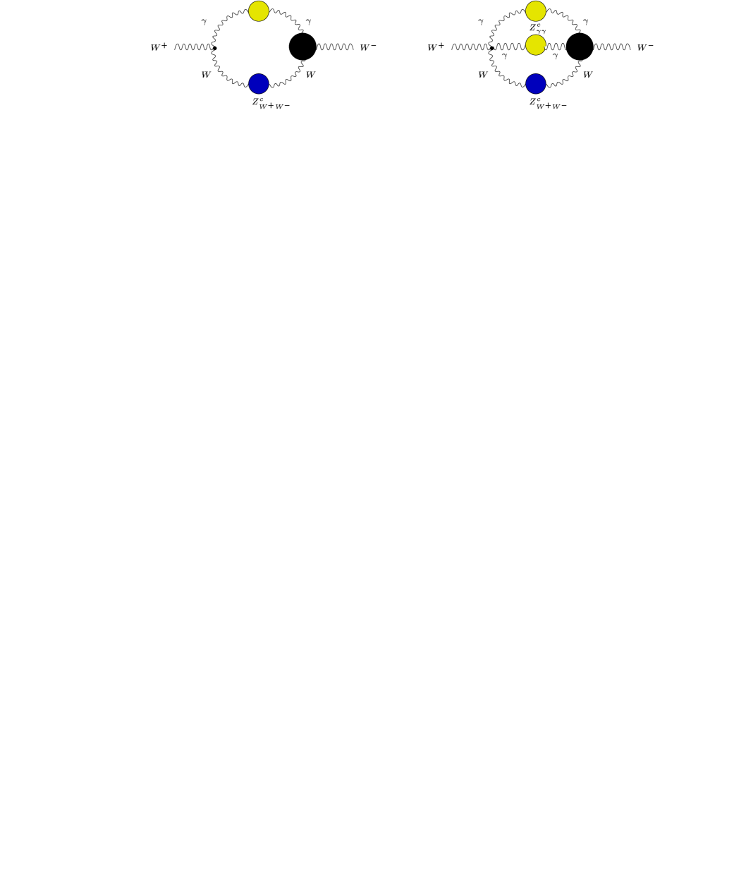
Figure 3: Schwinger-Dyson equation for the $W$ two-point function. The blobs on the internal lines represent connected propagators (chains of bubbles), while the blob on the vertex represents a one-particle irreducible Green function.

Diagrams with gauge-dependent threshold (like those with a charged Goldstone boson in place of the $W$) and with thresholds far away from the resonance region (like those with a $Z^{0}$ boson instead of the photon) can be discarded because their expansion around $s=M_{\scriptscriptstyle W}^{2}$ does not contain non-analytic terms.

We will treat explicitly only the case of the topology on the left side of Fig. 3, as the other diagram can be discussed along the same lines. In this case the Schwinger-Dyson equation has the form

$${\bf\Gamma}^{(\gamma)}_{{\scriptscriptstyle W}^{+}_{\mu}{\scriptscriptstyle W}^{-}_{\nu}}(p)\sim\int d^{n}k\ {\bf\Gamma}^{(0)}_{{\scriptscriptstyle W}^{+}_{\mu}A_{\rho}{\scriptscriptstyle W}^{-}_{\sigma}}(k,p+k)\,Z^{c}_{{\scriptscriptstyle A}_{\sigma}{\scriptscriptstyle A}_{\beta}}(k)\,Z^{c}_{{\scriptscriptstyle W}^{+}_{\sigma}{\scriptscriptstyle W}^{-}_{\alpha}}(k+p)\,{\bf\Gamma}_{{\scriptscriptstyle W}^{+}_{\alpha}A_{\beta}{\scriptscriptstyle W}^{-}_{\nu}}(k,p),$$ (20)

where ${\bf\Gamma}^{(\gamma)}_{{\scriptscriptstyle W}^{+}_{\mu}{\scriptscriptstyle W}^{-}_{\nu}}(p)$ is the contribution to the self-energy due to the exchange of a single photon, ${\bf\Gamma}_{{\scriptscriptstyle W}^{+}_{\mu}A_{\rho}{\scriptscriptstyle W}^{-}_{\sigma}}(k,p+k)$ is the 1PI vertex, the superscript $(0)$ indicates that the vertex is considered at the tree level, and finally $Z^{c}_{{\scriptscriptstyle A}_{\sigma}{\scriptscriptstyle A}_{\beta}}(k)$ and $Z^{c}_{{\scriptscriptstyle W}^{+}_{\sigma}{\scriptscriptstyle W}^{-}_{\alpha}}(k+p)$ are the connected propagator for the photon and for the $W$ boson, respectively. To study the IR behavior of Eq. (20) near the mass-shell, we now consider the transverse part of the self-energy ${\bf\Gamma}^{(\gamma)}_{{\scriptscriptstyle W}^{+}_{\mu}{\scriptscriptstyle W}^{-}_{\nu}}(p)$ and approach the limit $p^{2}\rightarrow\bar{s}_{\scriptscriptstyle W}$. We expand the propagator into the Dyson series of self-energies and tree propagators. Concerning the photon line, we recall that a convenient choice of the normalization conditions for the neutral gauge boson sector, i.e. ${\bf\Gamma}^{\scriptscriptstyle T}_{{\scriptscriptstyle Z}{\scriptscriptstyle A}}(0)=0$, makes ${\bf\Gamma}_{{\scriptscriptstyle A}{\scriptscriptstyle A}}^{\scriptscriptstyle T}(0)$ vanish at all orders (Cf. next section). Therefore, the photon propagator $Z^{c}_{{\scriptscriptstyle A}_{\sigma}{\scriptscriptstyle A}_{\tau}}(k)$ is always proportional to $1/k^{2}$ in the limit $k\rightarrow 0$ and has IR dimension -2.

For what concerns the $W$ propagator, the IR divergent contributions are related only to the transverse component of $Z^{c}_{{\scriptscriptstyle W}^{+}{\scriptscriptstyle W}^{-}}(k+p)$ because the propagator of the longitudinal components of the $W$ boson has a gauge dependent pole. In the on-shell limit for the momentum $p$ and for $k\rightarrow 0$, the tree level $W$ propagators present in the Dyson series for $Z^{c,{\scriptscriptstyle T}}_{{\scriptscriptstyle W}^{+}{\scriptscriptstyle W}^{-}}(k+p)$ are linearly divergent. Therefore, expanding $Z^{c,{\scriptscriptstyle T}}_{{\scriptscriptstyle W}^{+}{\scriptscriptstyle W}^{-}}(k+p)$ around $k=0,p^{2}=\bar{s}_{\scriptscriptstyle W}$ we have

$$\left.Z^{c,{\scriptscriptstyle T}}_{{\scriptscriptstyle W}^{+}{\scriptscriptstyle W}^{-}}(k+p)\right|_{p^{2}=\bar{s}_{\scriptscriptstyle W}}\stackrel{{\scriptstyle k\rightarrow 0}}{{\sim}}\,\sum_{n}\left(\frac{1}{2p\cdot k}\right)^{n+1}\left[{\bf\Gamma}^{{\scriptscriptstyle T}}_{{\scriptscriptstyle W}{\scriptscriptstyle W}}(\bar{s}_{\scriptscriptstyle W})\right]^{n}.$$ (21)

Here we consider only the most dangerous terms, which vanish if and only if ${\bf\Gamma}^{{\scriptscriptstyle T}}_{{\scriptscriptstyle W}{\scriptscriptstyle W}}(\bar{s}_{\scriptscriptstyle W})=0$. Under this condition, $\left.Z^{c,{\scriptscriptstyle T}}_{{\scriptscriptstyle W}^{+}{\scriptscriptstyle W}^{-}}(k+p)\right|_{p^{2}=\bar{s}_{\scriptscriptstyle W}}$ is at most linearly divergent in the IR limit. If, on the other hand, Eq. (17) is not satisfied, severe IR divergences appear in each order. The situation is not much improved if we move off the pole position in the resonance region. Indeed, in this case the $W$ width acts as an IR regulator in the denominator of Eq. (21), but leads to a series where the denominator $1/(s-\bar{s}_{\scriptscriptstyle W})\approx O(1/g^{2})$ spoils the convergence of the perturbative expansion in the resonance region [10].

The last information we need concerns the behavior of the vertex ${\bf\Gamma}^{{\scriptscriptstyle T}}_{{\scriptscriptstyle W}^{+}{\scriptscriptstyle A}_{\beta}{\scriptscriptstyle W}^{-}}(k,p)$ ($T$ refers to the transverse components of the $W$ bosons) around $k=0,p^{2}=M_{\scriptscriptstyle W}^{2}$. By analyticity and dimensional analysis, the vertex functions can be at most logarithmically divergent in the limit $k\rightarrow 0$ (this can also be verified exploiting the STI together with a proper use of the renormalization conditions). Having IR dimension -3, it follows by power counting that Eq. (20) does not lead to IR divergences when the integral in the internal momentum $k$ is performed around $k=0$.

In summary, we have seen that the pole mass of the $W$ boson, defined by Eq. (17), is IR safe to all orders in perturbation theory and that only if this definition is adopted a perturbative description of the resonance region is possible.

5 The $Z-\gamma$ system

The main difference between the case of the $W$ boson and the one of the neutral vector bosons is the presence of mixing. We now directly use Eq. (5) with $\beta^{\xi}_{i}=0$ and set $\rho^{\xi}=0$ for ease of notation (doing otherwise would not modify our results). Following the same steps as in the derivation of Eq. (16), and keeping in mind that the abelian vector field does not need a BRST source, we find for $i,j=A,Z$

$$\partial_{\xi}{\bf\Gamma}_{ij}^{{\scriptscriptstyle T}}(s) = -\left({\bf\Gamma}_{\chi\gamma_{3}i}^{\scriptscriptstyle T}(s)-\gamma^{\xi}_{i3}\right)\left[c_{\scriptscriptstyle W}{\bf\Gamma}_{{\scriptscriptstyle Z}j}^{\scriptscriptstyle T}(s)-s_{\scriptscriptstyle W}{\bf\Gamma}_{{\scriptscriptstyle A}j}^{\scriptscriptstyle T}(s)\right]$$ (22)

$$-\Big{[}c_{\scriptscriptstyle W}{\bf\Gamma}_{i{\scriptscriptstyle Z}}^{\scriptscriptstyle T}(s)-s_{\scriptscriptstyle W}{\bf\Gamma}_{i{\scriptscriptstyle A}}^{\scriptscriptstyle T}(s)\Big{]}\left({\bf\Gamma}_{\chi\gamma_{3}j}^{\scriptscriptstyle T}(s)-\gamma^{\xi}_{3j}\right),$$

where $\gamma^{\xi}_{i3}=\gamma^{\xi}_{3i}$ is the deformation induced by the possible mismatch between the wave function renormalization matrix $Z_{ij}$ and the renormalization of ${\bf\Gamma}_{\chi\gamma_{3}j}$. We recall that ${\bf\Gamma}_{ik}^{\scriptscriptstyle T}(s)$ is a symmetric matrix. We now consider the quantity

$${\cal D}_{{\scriptscriptstyle A}{\scriptscriptstyle Z}}^{\scriptscriptstyle T}(s)=\det\left(\begin{array}[]{ll}{\bf\Gamma}_{{\scriptscriptstyle A}{\scriptscriptstyle A}}^{{\scriptscriptstyle T}}(s)&{\bf\Gamma}_{{\scriptscriptstyle A}{\scriptscriptstyle Z}}^{{\scriptscriptstyle T}}(s)\\ {\bf\Gamma}_{{\scriptscriptstyle Z}{\scriptscriptstyle A}}^{{\scriptscriptstyle T}}(s)&{\bf\Gamma}_{{\scriptscriptstyle Z}{\scriptscriptstyle Z}}^{{\scriptscriptstyle T}}(s)\end{array}\right),$$ (23)

which appears in the denominator of the propagators of the photon-$Z^{0}$ system (see for ex. [33]). If we are interested in the analytic structure of neutral current amplitudes in the typical configuration of a high-energy collider, where external fermion masses can be neglected, ${\cal D}_{{\scriptscriptstyle A}{\scriptscriptstyle Z}}^{\scriptscriptstyle T}(s)$ is what we need to investigate. It is straightforward to derive

$$\partial_{\xi}{\cal D}_{{\scriptscriptstyle A}{\scriptscriptstyle Z}}^{\scriptscriptstyle T}(s)=-2\left(c_{\scriptscriptstyle W}{\bf\Gamma}_{\chi\gamma_{3}{\scriptscriptstyle Z}}^{\scriptscriptstyle T}(s)-c_{\scriptscriptstyle W}\gamma^{\xi}_{3{\scriptscriptstyle Z}}-s_{\scriptscriptstyle W}{\bf\Gamma}_{\chi\gamma_{3}{\scriptscriptstyle A}}^{\scriptscriptstyle T}(s)-s_{\scriptscriptstyle W}\gamma^{\xi}_{3{\scriptscriptstyle A}}\right){\cal D}_{{\scriptscriptstyle A}{\scriptscriptstyle Z}}^{\scriptscriptstyle T}(s).$$ (24)

This tells us that the zeros of ${\cal D}_{{\scriptscriptstyle A}{\scriptscriptstyle Z}}^{\scriptscriptstyle T}$ identify gauge-independent quantities. On the other hand, we know from the STI that ${\cal D}_{{\scriptscriptstyle A}{\scriptscriptstyle Z}}^{\scriptscriptstyle L}(0)=0$ (see for ex. [32]; Ref. [16] considers also the case of CP violation) which in turn implies by analyticity ${\cal D}_{{\scriptscriptstyle A}{\scriptscriptstyle Z}}^{\scriptscriptstyle T}(0)=0$. This result ensures the existence of a massless state, the photon. ${\cal D}_{{\scriptscriptstyle A}{\scriptscriptstyle Z}}^{\scriptscriptstyle T}$ has, however, another zero, corresponding to the $Z^{0}$ complex pole, at $q^{2}=\bar{s}_{\scriptscriptstyle Z}$. As in the case of the $W$ boson, this result implies that the position of the complex pole is a gauge independent quantity and that the only self-consistent normalization condition for the $Z^{0}$ mass is the one given in analogy to Eq. (17). With the exception of the IR problems, all the discussion on the $W$ mass applies directly to the case of the $Z^{0}$ boson mass [8]. A Ward Identity similar to the Nielsen identity of Eq. (16) has been applied in [9] to the case of the $Z^{0}$ resonance, to the same avail.

Another interesting application of Eq. (22) concerns the photon correlator at $q^{2}=0$. As is well known [32], using the renormalization condition ${\bf\Gamma}^{\scriptscriptstyle T}_{{\scriptscriptstyle A}{\scriptscriptstyle Z}}(0)=0$ the result ${\cal D}^{\scriptscriptstyle T}_{{\scriptscriptstyle A}{\scriptscriptstyle Z}}(0)$ that we have used above implies ${\bf\Gamma}_{{\scriptscriptstyle A}{\scriptscriptstyle A}}^{\scriptscriptstyle T}(0)=0$. In this case it is straightforward to verify from Eq. (22) that the derivative wrt $q^{2}$ of the photon two-point function calculated at $q^{2}=0$ is gauge-independent at all orders. Imposing the condition ${\bf\Gamma}^{\scriptscriptstyle T}_{{\scriptscriptstyle A}{\scriptscriptstyle Z}}(0)=0$ in the expression of $\partial_{\xi}{\bf\Gamma}^{\scriptscriptstyle T}_{{\scriptscriptstyle A}{\scriptscriptstyle Z}}(0)$, we obtain the constraint ${\bf\Gamma}^{\scriptscriptstyle T}_{\chi\gamma_{3}{\scriptscriptstyle A}}(0)-\gamma^{\xi}_{3{\scriptscriptstyle A}}=0$. We can now differentiate $\partial_{\xi}{\bf\Gamma}_{{\scriptscriptstyle A}{\scriptscriptstyle A}}^{\scriptscriptstyle T}$ wrt $s$ and evaluate it at $s=0$. Using the various constraints we have obtained, we immediately derive

$$\partial_{\xi}\,\left.\frac{\partial}{\partial{s}}{\bf\Gamma}_{{\scriptscriptstyle A}{\scriptscriptstyle A}}^{\scriptscriptstyle T}(s)\right|_{s=0}=0.$$ (25)

Notice that no particular renormalization condition on the derivative $\frac{\partial}{\partial{s}}{\bf\Gamma}_{{\scriptscriptstyle A}{\scriptscriptstyle A}}^{\scriptscriptstyle T}|_{s=0}$ has been imposed, so one should think, for instance, of a minimal subtraction. This interesting and non-trivial result shows that under the condition ${\bf\Gamma}^{\scriptscriptstyle T}_{{\scriptscriptstyle A}{\scriptscriptstyle Z}}(0)=0$ and at $s=0$ there exists in the full SM something analogous to what happens in QED, where the vacuum polarization of the photon is gauge-independent for any $s$ (see for ex. Ref.[37]). An alternative derivation of Eq. (25) can be obtained starting from the physical photon-electron amplitude at $s=0$, proceeding along the lines of the discussion of Sec. 8, and taking the gauge-independence of the on-shell amplitude for granted.

6 The scalar sector

In the previous section we have studied a first example of mixing. Indeed, mixing occurs in several other cases in the SM and in most of its extensions; all can be treated in a way very similar to the $\{\gamma,Z\}$ case discussed above. In this section, we first consider the matrix ${\bf\Gamma}^{\phi}(s)$ of the two point functions relative to the scalar fields $\phi=\{\phi_{1},\phi_{2},...,\phi_{n}\}$ in the general case of mixing and show that the gauge dependence of its determinant follows an equation analogous to Eq. (24), if the rank of ${\bf\Gamma}^{\phi}(s)$ is equal to its dimension $n$. As CP violation is present in the SM, we then consider the system formed by $\{A_{\scriptscriptstyle L},Z_{\scriptscriptstyle L},G_{0},H\}$, where the subscript $L$ denotes the longitudinal component of the vector boson fields. This system is highly constrained by the STI and we show that in this case the complex pole of the only physical field, the Higgs boson, is gauge-invariant. In an analogous way one can consider the $\{W_{\scriptscriptstyle L}^{\pm},G^{\pm}\}$ system, which however has no physical degree of freedom and is completely constrained by the STI.

The general form of the Nielsen identity in the case of a system $\phi$ of fields characterized by the same conserved quantum numbers can be obtained in analogy to Eq. (22) and reads

$$\partial_{\xi}{\bf\Gamma}^{\phi}(s)=\Lambda(s)\,{\bf\Gamma}^{\phi}(s)+{\bf\Gamma}^{\phi}(s)\,\Lambda^{\prime}(s),$$ (26)

where we do not need to specify the matrices $\Lambda$ and $\Lambda^{\prime}$ any further. Using $\ln\,\det{\bf\Gamma}^{\phi}={\rm tr}\,\ln{\bf\Gamma}^{\phi}$ and exploiting the properties of the trace, one finds for ${\cal D}_{\phi}\equiv\det{\bf\Gamma}^{\phi}$

$$\partial_{\xi}{\cal D}_{\phi}(s)={\rm tr}\left[\Lambda(s)+\Lambda^{\prime}(s)\right]{\cal D}_{\phi}(s),$$ (27)

which generalizes Eq. (24) in the case the rank of ${\bf\Gamma}^{\phi}(s)$ at arbitrary $s$ is equal to its dimensionality. In the case of $n$ scalar fields this ensures the gauge-independence of $n$ complex poles. Notice that the physical information contained in the matrix ${\bf\Gamma}^{\phi}$ is not restricted to the physical poles. Indeed, the higher order definition of the mixing parameters is affected by the off-diagonal elements of ${\bf\Gamma}^{\phi}$. In general, it does not seem possible to form gauge-independent quantities on the basis of two-point functions only, i.e. of ${\bf\Gamma}^{\phi}$, and to employ them to renormalize the mixing parameters [15]. On the other hand, the mixing parameters can be safely defined in terms of physical observables such as mesonic decay rates.

Neutral current processes are mediated by photons and $Z^{0}$, as well as by scalar fields, like $G_{0}$ and the physical Higgs. As it is well-known, the propagator matrix is obtained by inversion of the two-point function matrix and, in the process of inversion, the transverse and longitudinal components of the vector boson fields decouple. Having considered the transverse degrees of freedom in the preceding section, we can now limit ourselves to the system formed by the longitudinal components of the photon and of the $Z^{0}$ and by the Higgs and the neutral Goldstone bosons, which we denote by $S=\{A_{\scriptscriptstyle L},Z_{\scriptscriptstyle L},G_{0},H\}$. The two point functions involving one vector boson and one scalar are defined extracting $q^{\mu}$. In this way, ${\bf\Gamma}^{S}$ is the 4$\times$4 matrix of the two-point functions of $S$.

The system $S$ includes unphysical degrees of freedom. As we have noted in the introduction, even at the tree level the Green functions of unphysical fields are modified by the choice to use the reduced generating functional ${\bf\Gamma}$ in place of the complete functional ${{\bf\Gamma}^{c}}$ (see the App. A). For the purposes of this section, however, the reduced functional simplifies significantly the derivation without affecting the physical information we can extract from ${\bf\Gamma}^{S}$. In a way, this can be viewed as a consequence of the fact that the cancellation between the unphysical degrees of freedom occurs independently of the gauge-fixing sector [32, 20].

Each row of ${\bf\Gamma}^{S}$ is connected by a STI. For instance, differentiating Eq. (A3) with respect to $A^{\mu}$ and $c^{\scriptscriptstyle A}$, we obtain for the first row

$$\left(c^{2}_{\scriptscriptstyle W}-s_{\scriptscriptstyle W}{\bf\Gamma}_{c_{\scriptscriptstyle A}\gamma_{3}}\right){\bf\Gamma}_{{\scriptscriptstyle A}{\scriptscriptstyle A}}^{\scriptscriptstyle L}+\left(s_{\scriptscriptstyle W}c_{\scriptscriptstyle W}+c_{\scriptscriptstyle W}{\bf\Gamma}_{c_{\scriptscriptstyle A}\gamma_{3}}\right){\bf\Gamma}_{{\scriptscriptstyle A}{\scriptscriptstyle Z}}^{\scriptscriptstyle L}+{\bf\Gamma}_{{\scriptscriptstyle A}{\scriptscriptstyle G}_{0}}{\bf\Gamma}_{c_{\scriptscriptstyle A}\gamma_{0}}+{\bf\Gamma}_{{\scriptscriptstyle A}{\scriptscriptstyle H}}{\bf\Gamma}_{c_{\scriptscriptstyle A}\gamma_{\scriptscriptstyle H}}=0.$$ (28)

Similar identities can be derived for the other rows, so that the STI for the two-point functions can be written as ${\bf\Gamma}^{S}V_{c_{\scriptscriptstyle A}}=0$, where $V_{c_{\scriptscriptstyle A}}^{\scriptscriptstyle T}=(c^{2}_{\scriptscriptstyle W}-s_{\scriptscriptstyle W}{\bf\Gamma}_{c_{\scriptscriptstyle A}\gamma_{3}},s_{\scriptscriptstyle W}c_{\scriptscriptstyle W}+c_{\scriptscriptstyle W}{\bf\Gamma}_{c_{\scriptscriptstyle A}\gamma_{3}},{\bf\Gamma}_{c_{\scriptscriptstyle A}\gamma_{0}},{\bf\Gamma}_{c_{\scriptscriptstyle A}\gamma_{\scriptscriptstyle H}})$. Since $\phi$ includes the unphysical components of the photon and $Z^{0}$ fields and since we have eliminated the gauge fixing sector of the tree level Lagrangian in using the reduced functional (see Eq. (A2)), it is perhaps not surprising that there is no propagator for $A_{\scriptscriptstyle L}$ and $Z_{\scriptscriptstyle L}$ and that $\det{\bf\Gamma}^{S}=0$ or the rank of ${\bf\Gamma}^{S}$ is less than 4. In fact, ${\bf\Gamma}^{S}$ has another linearly independent eigenvector $V_{c_{\scriptscriptstyle Z}}$ with zero eigenvalue, corresponding to the set of STI obtained by differentiation wrt $c_{\scriptscriptstyle Z}$. Therefore, the rank of ${\bf\Gamma}^{S}$ is at most 2 and that we cannot use Eq. (27) at this stage. Moreover, the sub-matrix of ${\bf\Gamma}^{S}$ identified by the indices $G_{0}$ and $H$ has the same rank as ${\bf\Gamma}^{S}$. This can be seen by noting that $V_{c_{\scriptscriptstyle Z}}$ and $V_{c_{\scriptscriptstyle A}}$ can be orthogonalized in the subspace of the $A^{\scriptscriptstyle L}$ and $Z^{\scriptscriptstyle L}$ components because

$$\det\left(\begin{array}[]{ll}c^{2}_{\scriptscriptstyle W}-s_{\scriptscriptstyle W}{\bf\Gamma}_{c_{\scriptscriptstyle A}\gamma_{3}}&s_{\scriptscriptstyle W}c_{\scriptscriptstyle W}-s_{\scriptscriptstyle W}{\bf\Gamma}_{c_{\scriptscriptstyle Z}\gamma_{3}}\\ s_{\scriptscriptstyle W}c_{\scriptscriptstyle W}+c_{\scriptscriptstyle W}{\bf\Gamma}_{c_{\scriptscriptstyle A}\gamma_{3}}&s^{2}_{\scriptscriptstyle W}+c_{\scriptscriptstyle W}{\bf\Gamma}_{c_{\scriptscriptstyle Z}\gamma_{3}}\end{array}\right)=1+O(\hbar)\neq 0,$$ (29)

Having eliminated the unphysical longitudinal components of the vector bosons, we can now concentrate on the sub-matrix

$${\bf\Gamma}^{\cal H}=\left(\begin{array}[]{ll}{\bf\Gamma}_{G_{0}G_{0}}&{\bf\Gamma}_{G_{0}H}\\ {\bf\Gamma}_{HG_{0}}&{\bf\Gamma}_{HH}\\ \end{array}\right),$$ (30)

whose rank is equal to the one of ${\bf\Gamma}^{S}$. Indeed, at arbitrary $q^{2}$, its rank is 2, so that Eq. (27) is satisfied. ${\bf\Gamma}^{\cal H}$ is very similar to the $\gamma-Z^{0}$ transverse mixing matrix. Even if the CP violation mixes up physical and unphysical scalar fields at high perturbative orders, it is not difficult to disentangle them taking advantage of the STI. At $q^{2}=0$ the two STI obtained by differentiating wrt $c_{{\scriptscriptstyle A},{\scriptscriptstyle Z}}$ and $G_{0}$ imply that $\det{\bf\Gamma}^{\cal H}(0)=0$. This zero is related to the $G^{0}$ field and is located at $q^{2}=0$ (in the standard $R_{\xi}$ gauge it would be at $q^{2}=\xi_{\scriptscriptstyle Z}M_{\scriptscriptstyle Z}^{2}$) as a consequence of the use of the reduced functional. The remaining zero, at $q^{2}=\bar{s}_{\scriptscriptstyle H}$, corresponds instead to the physical pole of the Higgs boson and its location in the complex plane is therefore gauge-independent, as it follows from Eq. (27). A discussion of the relation between the pole mass and the conventionally renormalized mass of the Higgs boson in this case can be found in Ref.[38].

7 Fermions

The treatment of the fermionic sector is only slightly more involved than that of the scalar sector. Again, we consider the most general case of mixing and call ${\bf\Gamma}^{f}$ the matrix of the fermionic two-point functions, ${\bf\Gamma}_{\bar{f}f^{\prime}}$. In the case of massless neutrinos, there is no mixing in the leptonic sector and ${\bf\Gamma}^{lept}$ is a diagonal matrix. As a first step, we need to decompose ${\bf\Gamma}^{f}$ into scalar pieces:

$${\bf\Gamma}^{f}(p)=\Sigma_{{\scriptscriptstyle L}}(p^{2})\not\!p\,P_{{\scriptscriptstyle L}}+\Sigma_{{\scriptscriptstyle R}}(p^{2})\not\!p\,P_{{\scriptscriptstyle R}}+\Sigma_{{\scriptscriptstyle D}}(p^{2})P_{{\scriptscriptstyle L}}+\Sigma_{{\scriptscriptstyle D}}^{\dagger}(p^{2})P_{{\scriptscriptstyle R}}$$ (31)

where $P_{{\scriptscriptstyle L},{\scriptscriptstyle R}}=\frac{1}{2}(1\mp\gamma_{5})$ are the left and right-handed projectors. As can be seen by inverting ${\bf\Gamma}^{f}$, the relevant quantity for the fermion propagator matrix is the matrix [39]

$${K_{f}}(p^{2})=p^{2}\,\Sigma_{{\scriptscriptstyle L}}-\Sigma_{{\scriptscriptstyle D}}^{\dagger}\,\,\Sigma_{{\scriptscriptstyle R}}^{-1}\,\Sigma_{{\scriptscriptstyle D}},$$ (32)

where we have dropped the $p^{2}$ dependence of the $\Sigma$ matrices. Since the determinant of this matrix appears in the denominator of the fermion propagators, we want to study its zeros, i.e. the zeros of the eigenvalues of $K_{f}$. We recall that by pseudo-hermiticity ${\bf\Gamma}^{f}=\gamma^{\dagger}_{0}\,{{\bf\Gamma}}^{f\dagger}\,\gamma_{0}$, so that $\Sigma_{{\scriptscriptstyle L}}^{\dagger}(p^{2})=\Sigma_{{\scriptscriptstyle L}}(p^{2})$ and $\Sigma_{{\scriptscriptstyle R}}^{\dagger}(p^{2})=\Sigma_{{\scriptscriptstyle R}}(p^{2})$ (this is actually true below thresholds, but it does not affect our conclusions). Hence, the matrix ${K}_{f}(p^{2})$ is hermitian and can be diagonalized by means of a unitary transformation. Under the usual assumption $\beta_{i}^{\xi}=0$, the gauge-parameter dependence of ${\bf\Gamma}^{f}$ is described by a Nielsen identity which has exactly the same form of Eq. (26). Setting furthermore $\rho^{\xi}=\gamma^{\xi}_{\varphi}=0$ for ease of notation (the results would not change), we have $\Lambda=-{\bf\Gamma}_{\chi\bar{f}\eta_{f^{\prime}}}$ and $\Lambda^{\prime}=-{\bf\Gamma}_{\chi\bar{\eta}_{f}f^{\prime}}$, which have a Dirac structure and undergo a decomposition analogous to Eq. (31). Again by pseudo-hermiticity, we find that in this case $\Lambda_{{\scriptscriptstyle L},{\scriptscriptstyle R}}=(\Lambda^{\prime}_{{\scriptscriptstyle L},{\scriptscriptstyle R}})^{\dagger}$ and $\Lambda_{\scriptscriptstyle D}=\Lambda^{\prime}_{\scriptscriptstyle D}$. It is then straightforward to verify that the components of ${\bf\Gamma}^{f}$ satisfy

$$\partial_{\xi}\Sigma_{{\scriptscriptstyle L}} = {\Lambda}_{{\scriptscriptstyle L}}\Sigma_{{\scriptscriptstyle D}}+\Sigma_{{\scriptscriptstyle L}}{\Lambda}_{{\scriptscriptstyle D}}+{\Lambda}_{{\scriptscriptstyle D}}^{\dagger}\Sigma_{{\scriptscriptstyle L}}+\Sigma_{{\scriptscriptstyle D}}^{\dagger}{\Lambda}_{{\scriptscriptstyle L}}^{\dagger}$$

$$\partial_{\xi}\Sigma_{{\scriptscriptstyle R}} = {\Lambda}_{{\scriptscriptstyle D}}\Sigma_{{\scriptscriptstyle R}}+\Sigma_{{\scriptscriptstyle R}}{\Lambda}_{{\scriptscriptstyle D}}^{\dagger}+{\Lambda}_{{\scriptscriptstyle R}}\Sigma_{{\scriptscriptstyle D}}^{\dagger}+\Sigma_{{\scriptscriptstyle D}}{\Lambda}_{{\scriptscriptstyle R}}^{\dagger}$$ (33)

$$\partial_{\xi}\Sigma_{{\scriptscriptstyle D}} = p^{2}({\Lambda}_{{\scriptscriptstyle R}}\Sigma_{{\scriptscriptstyle L}}+\Sigma_{{\scriptscriptstyle R}}{\Lambda}_{{\scriptscriptstyle L}}^{\dagger})+\Lambda_{\scriptscriptstyle D}\Sigma_{\scriptscriptstyle D}+\Sigma_{\scriptscriptstyle D}\Lambda_{\scriptscriptstyle D}\ ,$$

from which it follows that

$$\partial_{\xi}{K_{f}}={K_{f}}\,F+F^{\dagger}\,K_{f}\,,$$ (34)

with $F=\Lambda_{\scriptscriptstyle D}-\Lambda_{\scriptscriptstyle R}^{\dagger}\Sigma_{\scriptscriptstyle R}^{-1}\Sigma_{\scriptscriptstyle D}$. Without using pseudo-hermiticity, we would have $F^{\prime}\neq F^{\dagger}$ in place of $F^{\dagger}$ in the previous equation. Eq. (34) is in the form of Eq. (26) and therefore ${\cal D}_{f}\equiv\det K_{f}$ satisfies Eq. (27). We have therefore algebraically reduced the problem in the fermionic case to the scalar one. In the case of mixing between $n$ fermions, the gauge-parameter independence of $n$ complex poles is thus warranted. Again, this result holds for any choice of the fermion wave function renormalization and relies solely on the $\beta^{\xi}_{i}=0$ assumption.

The above proof is new and valid in the full SM. For what concerns pure QED and QCD, the result that the pole masses of the electron and of the quark are gauge-independent is not new and has been obtained both using the Nielsen identities [37] and in different ways [11, 40]. In QED (QCD) the situation simplifies considerably: writing ${\bf\Gamma}_{\bar{f}f}=B\not\!p-mA$, where $m$ is the mass of the electron (quark), and decomposing $\Lambda$ in an analogous way, we find

$$-\partial_{\xi}A=\frac{p^{2}}{m}\,B\,\Lambda_{\scriptscriptstyle B}+m\,A\,\Lambda_{\scriptscriptstyle A};\ \ \ \ -\partial_{\xi}B={m}\left(A\,\Lambda_{\scriptscriptstyle B}+B\,\Lambda_{\scriptscriptstyle A}\right),$$ (35)

which could be tested up to $O(\alpha_{s}^{2})$ against the general $R_{\xi}$ gauge calculation of Ref.[41].

The proof of the IR finiteness of the fermions in the SM follows Ref.[11] and the final discussion in Sec. 3 and is already present in nuce in Ref.[10]. For completeness, in App. B we present the explicit gauge-parameter dependence of the one-loop fermionic self-energies in a general $R_{\xi}$ gauge for the full SM. Remembering that $\Lambda$ first occur at the one-loop level, it is straightforward to see that they satisfy the Nielsen identities Eq. (7). This completes the set of expressions given in Ref.[13] and is very useful in particular applications. For instance, Eqs. (C1-C3) have been used in Ref.[15] to discuss the gauge dependence of the one-loop definition of the CKM matrix. Indeed, as noted in the previous section, the renormalization of the mixing parameters is a delicate subject for what concerns the gauge-parameter dependence. An adequate framework for studying it is the Background Field Method [16]. In the case of the fermion mixing a comprehensive analysis has been presented in Ref.[15].

8 Application to physical amplitudes

In this section we apply the formalism of the Nielsen identities to four-fermion physical amplitudes and study the mechanism of gauge cancellations at any order in perturbation theory. Our purpose here is not to prove the gauge-independence of the physical amplitudes, a result which was accomplished in full generality long ago at the level of the generating functional [25]. We would rather like to study a specific example and carry out the analysis at an arbitrary order in perturbation theory. The use of the Nielsen identities allows us to uncover the regularities of the gauge recombinations between the different components (vertices, boxes and self-energies) in great generality. The following derivation is formally independent of the perturbative expansion of the Green functions. In other words, if we work at order $n$ in perturbation theory the Green functions have to be expanded up to this order, but the factorization works independently of that. At the one-loop level, a similar factorization is also accomplished diagrammatically by the Pinch Technique (PT) [42], whose extension at higher orders has however proved problematic. Unlike the PT, the Nielsen identities control only the gauge parameter variation and cannot be used to construct explicitly gauge-independent proper functions which satisfy basic requirements and tree-level-like Ward identities. However, they may prove useful in the search for the higher-order extension of the PT. The analysis of this section gives us also the opportunity to present explicitly the Nielsen identities for vertices and boxes involving fermions, which are interesting in their own respect as they appear in most phenomenological applications.

We first consider the truncated Green function $Z^{trunc}_{\bar{I}J\bar{K}N}$ (see e.g. [26]) for a generic four fermion process $f_{\bar{I}}f_{J}\longrightarrow f_{\bar{K}}f_{N}$ and we decompose it in terms of irreducible diagrams and propagators. We will use capital and lowercase letters to denote fermions and bosonic fields (scalar as well as gauge vector bosons), respectively. Therefore, $Z^{c}_{\bar{I}J}$ and $Z^{c}_{ij}$ are the propagator functions of fermions and bosons. Following the convention of the preceding sections, irreducible boxes and vertices are denoted by ${\bf\Gamma}_{\bar{I}J\bar{K}N},{\bf\Gamma}_{\bar{I}Ji}$, and ${\bf\Gamma}_{j\bar{K}N}$. To keep the notation simple, we drop Lorentz indices and the dependence on the external momenta. The physical amplitude ${\cal M}_{\bar{I}J\bar{K}N}$ for our process is obtained from $Z^{trunc}_{\bar{I}J\bar{K}N}$ using the LSZ reduction formula [26], which in the case of fermion with mixing reads [32]

$${\cal M}_{\bar{I}J\bar{K}N}=\lim_{on-shell}{\widetilde{Z}}^{1/2}_{\bar{I}I^{\prime}}\,{\widetilde{Z}}^{1/2}_{\bar{J}^{\prime}J}\,\,Z^{trunc}_{\bar{I}^{\prime}J^{\prime}\bar{K}^{\prime}N^{\prime}}\,\,{\widetilde{Z}}^{1/2}_{\bar{K}K^{\prime}}\,{\widetilde{Z}}^{1/2}_{\bar{N}^{\prime}N},$$ (36)

where the on-shell limit includes the projection on the asymptotic states and $\widetilde{Z}$ controls the relation between the asymptotic states and the renormalized spinors:

$${\widetilde{Z}}^{1/2}_{\bar{I}J}\,u_{as,J}=u_{I}.$$ (37)

The matrix ${\widetilde{Z}}$ can be computed from the conditions [32] (quantum equations of motion)

$${\bf\Gamma}_{\bar{I}J}\,u_{J}(m_{J})=0;\ \ \ \ \ \bar{u}_{I}(m_{I})\,{\bf\Gamma}_{\bar{I}J}=0$$

$$\frac{\tilde{Z}_{II}}{\not\!p-m_{I}}\,{\bf\Gamma}_{\bar{I}I}\,u_{I}(m_{I})=u_{I}(m_{I});\ \ \ \bar{u}_{I}(m_{I})\,{\bf\Gamma}_{\bar{I}I}\,\frac{\tilde{Z}_{II}}{\not\!p-m_{I}}=\bar{u}_{I}(m_{I}),$$ (38)

using the fact that $(\not\!p-m_{J})\,u_{as}(m_{J})=0$ at any order by definition. Of course, $\widetilde{Z}$ should be decomposed in left and right-handed parts, $\widetilde{Z}=\widetilde{Z}^{\scriptscriptstyle L}P_{\scriptscriptstyle L}+\widetilde{Z}^{\scriptscriptstyle R}P_{\scriptscriptstyle R}$. Notice that the first line of Eqs. (38) implies $\det K_{f}=0$ and consequently includes the requirement that the mass parameters of the external fermions are renormalized on the poles of the propagators (see Sec. 7). Strictly speaking, the LSZ formalism applies only to stable external states, i.e.  to the electron and neutrinos and, to a good approximation, to the muon. Nevertheless, we will consider here the general case of mixing. We also stress that the LSZ factors $\widetilde{Z}$ should not be confused with the wave-function renormalization factors for the external fields. Of course, the latter can be chosen by imposing Eqs. (38) together with $\widetilde{Z}={\bf 1}$ (on-shell scheme [32]), but there is in general no restriction on their choice (see also [15]) and it is even possible to avoid them altogether, in which case $\widetilde{Z}$ is divergent. Once the wave-function renormalization has been defined, for instance through a minimal subtraction, the factors $\widetilde{Z}$ can be computed from Eqs. (38).

As a first step, we consider the gauge variation of the truncated Green function $Z^{trunc}_{\bar{I}J\bar{K}N}$ In the most general case of mixing, $Z^{trunc}_{\bar{I}J\bar{K}N}$ is decomposed in the following blocks (we sum over repeated indices)

$$Z^{trunc}_{\bar{I}J\bar{K}N} = i\,{\bf\Gamma}_{\bar{I}J\bar{K}N}-{\bf\Gamma}_{\bar{I}Ji}\ Z^{c}_{ij}\ {\bf\Gamma}_{j\bar{K}N}-{\bf\Gamma}_{\bar{I}Ni}\ Z^{c}_{ij}\ {\bf\Gamma}_{j\bar{K}J},$$ (39)

from which we obtain

$$\partial_{\xi}Z^{trunc}_{\bar{I}J\bar{K}N} = i\,\partial_{\xi}{\bf\Gamma}_{\bar{I}J\bar{K}N}$$

$$- \left(\partial_{\xi}{\bf\Gamma}_{\bar{I}Ji}\right)Z^{c}_{ij}\ {\bf\Gamma}_{j\bar{K}N}-{\bf\Gamma}_{\bar{I}Ji}\left(\partial_{\xi}Z^{c}_{ij}\right){\bf\Gamma}_{j\bar{K}N}-{\bf\Gamma}_{\bar{I}Ji}\ Z^{c}_{ij}\ \partial_{\xi}{\bf\Gamma}_{j\bar{K}N}$$

$$- \left(\partial_{\xi}{\bf\Gamma}_{\bar{I}Ni}\right)Z^{c}_{ij}\ {\bf\Gamma}_{j\bar{K}J}-{\bf\Gamma}_{\bar{I}Ni}\left(\partial_{\xi}Z^{c}_{ij}\right){\bf\Gamma}_{j\bar{K}J}-{\bf\Gamma}_{\bar{I}Ni}\ Z^{c}_{ij}\ \partial_{\xi}{\bf\Gamma}_{j\bar{K}J}\,.$$

We can compute the different contributions $\partial_{\xi}{\bf\Gamma}_{J\bar{I}N\bar{K}},\partial_{\xi}{\bf\Gamma}_{J\bar{I}i}$, and $\partial_{\xi}Z^{c}_{ij}$ using the Nielsen identities. The identity for the propagator functions $Z^{c}_{ij}$ and $Z^{c}_{\bar{I}J}$ is easily derived from the identity for the irreducible two-point functions ${\bf\Gamma}_{ij}$ and ${\bf\Gamma}_{\bar{I}J}$. As we have seen, the general form of the latter is

$$\partial_{\xi}{\bf\Gamma}_{ab}=-{\bf\Gamma}_{ac}\,{\bf\Gamma}_{\chi b\gamma_{c}}-{\bf\Gamma}_{\chi a\gamma_{c}}\,{\bf\Gamma}_{cb},$$ (41)

where the indices $a,b$ apply to both the bosonic and fermionic case. As usual, we employ the procedure of Sec. 2, remove all tadpoles, set $\delta_{t}=\delta_{t}^{CP}=0$, and assume $\beta^{\xi}_{i}=0,~{}\forall i$ (this is consistent with the LSZ use of pole masses, as we have seen). Concerning the $\rho^{\xi}$ and $\gamma^{\xi}_{\varphi}$ factors, we avoid them here in order to keep the formulas simple.

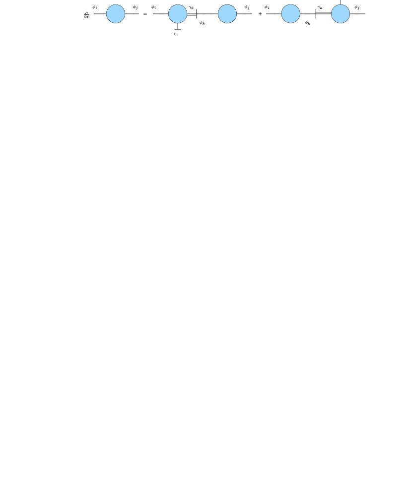
Figure 4: Nielsen identity for the two-point function ${\bf\Gamma}_{\phi_{i}\phi_{j}}$.

However, following the discussion in Sec. 2, they are bound to drop out of the amplitude and this can be explicitly verified. Eq. (41) can be graphically represented in the very simple way shown in Fig. 4. Notice that the momentum flows along the horizontal line and that the insertion of the static source $\chi$ does not carry momentum, unlike the one of $\gamma_{\varphi}$.

Using the relations $Z^{c}_{ij}\,{\bf\Gamma}_{jk}=i\delta_{ik}$ and $Z^{c}_{\bar{I}K}\,{\bf\Gamma}_{\bar{K}J}=i\delta_{IJ}{\bf 1}$, where ${\bf 1}$ is the identity matrix for the Dirac indices, we obtain the Nielsen identities for the propagator functions, which read

$$\partial_{\xi}Z^{c}_{ij} = Z^{c}_{ik}\,{\bf\Gamma}_{\chi k\gamma_{j}}+{\bf\Gamma}_{\chi\gamma_{i}k}\,Z^{c}_{kj},$$ (42)

$$\partial_{\xi}Z^{c}_{\bar{I}J} = Z^{c}_{\bar{I}K}{\bf\Gamma}_{\chi\bar{K}{\eta}_{J}}+{\bf\Gamma}_{\chi\bar{\eta}_{I}K}Z^{c}_{\bar{K}J},$$ (43)

for bosons and fermions, respectively. Graphically, these identities can be represented by Fig. 4 after replacing the blobs with the $\chi$ insertion by their mirror images and exchanging the corresponding indices. For the three-point functions we have

$$-\partial_{\xi}{\bf\Gamma}_{\bar{I}Ji} = {\bf\Gamma}_{\chi\gamma_{m}\bar{I}J}{\bf\Gamma}_{mi}+{\bf\Gamma}_{\chi i\gamma_{m}}{\bf\Gamma}_{m\bar{I}J}$$ (44)

$$+ {\bf\Gamma}_{\bar{I}Ki}{\bf\Gamma}_{\chi\bar{\eta}_{K}J}+{\bf\Gamma}_{\bar{I}K}{\bf\Gamma}_{\chi i\bar{\eta}_{K}J}+{\bf\Gamma}_{\chi\bar{I}{\eta}_{K}}{\bf\Gamma}_{\bar{K}Ji}+{\bf\Gamma}_{\chi i\bar{I}{\eta}_{K}}{\bf\Gamma}_{\bar{K}J}\,.$$

We see that the gauge-dependent terms of the form of ${\bf\Gamma}_{\chi\gamma_{i}j}$ introduced by the propagators in Eq. (8) are exactly cancelled by the last term in the first line of Eq. (44), i.e. by the vertices alone. Therefore, the boxes are not necessary to remove the gauge-dependence of the internal self-energies. The identity for the four-point functions is

$$-\partial_{\xi}{\bf\Gamma}_{\bar{I}J\bar{K}N} = {\bf\Gamma}_{\bar{I}Jm}\,{\bf\Gamma}_{\chi\gamma_{m}\bar{K}N}+{\bf\Gamma}_{\bar{I}Nm}\,{\bf\Gamma}_{\chi\gamma_{m}\bar{K}J}+{\bf\Gamma}_{\chi\gamma_{m}\bar{I}J}\,{\bf\Gamma}_{m\bar{K}N}+{\bf\Gamma}_{\chi\gamma_{m}\bar{I}N}\,{\bf\Gamma}_{m\bar{K}J}$$

$$+ {\bf\Gamma}_{\bar{I}S}\,{\bf\Gamma}_{\chi\bar{\eta}_{S}J\bar{K}N}+{\bf\Gamma}_{\bar{K}S}\,{\bf\Gamma}_{\chi\bar{I}J\bar{\eta}_{S}N}+{\bf\Gamma}_{\chi\bar{I}J\bar{K}{\eta}_{S}}\,{\bf\Gamma}_{\bar{S}N}+{\bf\Gamma}_{\chi\bar{I}{\eta}_{S}\bar{K}N}\,{\bf\Gamma}_{\bar{S}J}$$

$$+ {\bf\Gamma}_{\bar{I}J\bar{K}S}\,{\bf\Gamma}_{\chi\bar{\eta}_{S}N}+{\bf\Gamma}_{\bar{I}S\bar{K}N}\,{\bf\Gamma}_{\chi\bar{\eta}_{S}J}+{\bf\Gamma}_{\chi\bar{I}{\eta}_{S}}\,{\bf\Gamma}_{\bar{S}J\bar{K}N}+{\bf\Gamma}_{\chi\bar{K}{\eta}_{S}}\,{\bf\Gamma}_{\bar{I}J\bar{S}N}\,.$$

We now distinguish between the different Green functions containing the source $\chi$:

1. Terms of the form ${\bf\Gamma}_{\chi\gamma_{i}\bar{I}J}$ are present both in the gauge variation of the boxes (first line) and in the one of the vertices (first term). They cancel against each other in the sum (8) according to the pattern

   $$\underbrace{{\bf\Gamma}_{\chi\gamma_{m}\bar{I}J}\ {\bf\Gamma}_{mi}\ Z^{c}_{ij}\ {\bf\Gamma}_{j\bar{K}N}}_{-(\partial_{\xi}{\bf\Gamma}_{\bar{I}ji})\ Z^{c}_{ij}\ {\bf\Gamma}_{j\bar{K}N}}-\underbrace{i\,{\bf\Gamma}_{\chi\gamma_{m}\bar{I}J}\ {\bf\Gamma}_{m\bar{K}N}}_{i\,\partial_{\xi}{\bf\Gamma}_{\bar{I}J\bar{K}N}}=0\ ,$$

   where we have specified which part of Eq. (8) generates each term.

2. The factors containing ${\bf\Gamma}_{\chi i\bar{\eta}_{K}J}$ in the second line of Eq. (44) and ${\bf\Gamma}_{\chi\bar{\eta}_{S}J\bar{K}N}$ (the whole second line of Eq. (8)) always multiply a two-point function of the external fermions like ${\bf\Gamma}_{\bar{I}J}$. When they are contracted with the external spinors, these terms vanish, as a consequence of Eq. (38).

3. The remaining terms contain Green functions of the kind ${\bf\Gamma}_{\chi\bar{\eta}_{I}J}$ and ${\bf\Gamma}_{\chi\bar{I}\eta_{J}}$ which multiply vertices and boxes in Eqs. (44) and (8), respectively. As we will see in a moment, they are cancelled by the LSZ factors.

Adding together the various pieces, the gauge-parameter variation of the on-shell truncated Green function can be expressed in terms of the truncated function itself:

$$-\partial_{\xi}Z^{trunc}_{\bar{I}J\bar{K}N}|_{on-shell}={\bf\Gamma}_{\chi\bar{I}\eta_{S}}\,Z^{trunc}_{\bar{S}J\bar{K}N}+{\bf\Gamma}_{\chi\bar{K}\eta_{S}}\,Z^{trunc}_{\bar{I}J\bar{S}N}+Z^{trunc}_{\bar{I}S\bar{K}N}\,{\bf\Gamma}_{\chi\bar{\eta}_{S}J}+Z^{trunc}_{\bar{I}J\bar{K}S}\,{\bf\Gamma}_{\chi\bar{\eta}_{S}N},$$ (46)

according to the usual form for the Nielsen identities. Of course, this on-shell factorization holds in general for any amputated Green function, as it follows from the gauge independence of the $S$-matrix.

We are now ready to apply the LSZ reduction formula. The gauge variation of the factor $\widetilde{Z}$ can be computed from Eq. (37) and Eq. (38) using the Nielsen identities for the two-point functions and the gauge-independence of the asymptotic spinors $u_{as,I}$. We then obtain

$$\lim_{on-shell}\partial_{\xi}{\widetilde{Z}}^{1/2}_{\bar{I}J}\,u_{as,J}={\bf\Gamma}_{\chi\bar{I}\eta_{S}}{\widetilde{Z}}^{1/2}_{\bar{S}J}\,u_{as,J},$$ (47)

where ${\bf\Gamma}_{\chi\bar{I}\eta_{S}}$ is calculated on-shell, from which the final cancellation of the gauge-dependence follows.

If some of the $\beta^{\xi}_{i}$ do not vanish, the cancellations do not operate any longer and the amplitude turns out to be gauge parameter dependent [25]. An explicit example has been considered in [15], for the $W$ decay into quarks: if the CKM counterterm is gauge-dependent, the amplitude depends on the gauge parameters too. On the other hand, the above proof relies neither on a specific choice of renormalization of the unphysical parameters, nor on the regularization scheme adopted (provided the STI have been restored order by order).

9 Summary

We have introduced the Nielsen identities of the SM and used the problem of the definition of mass as a demonstrative example. In this context we have obtained some new results: we have proven to all orders in perturbation theory the gauge-parameter independence of the complex pole associated to any physical particle of the SM. We have considered the cases of the vector bosons, scalars and fermions in great generality, allowing for arbitrary mixing patterns. Particular attention has been paid to the case of the $W$ boson, which is simpler because of the absence of mixing and has been chosen to illustrate some features common to all cases. Most of the proofs hold without modifications also in some extensions of the SM, like non-supersymmetric two-Higgs-doublet models.

We have derived identities for the gauge-dependence of all the two-point functions of the SM, both for bosons and fermions, as well as for vertices and boxes involving external fermions. Using these expressions, we have shown the explicit mechanism of gauge cancellations which leads to gauge-independent four fermion amplitudes to all orders in the most general case of fermion and boson mixings and of CP violation. The formalism introduced in this paper, supplemented by the material given in App. A (the Lagrangian involving the BRST sources), should allow for a very simple derivation of the Nielsen identities for any proper Green function in the electroweak SM and in QCD.

We have also extensively discussed the renormalization of the Nielsen identities with an arbitrary regularization, in the case the Nielsen identities (but not the STI) are broken by renormalization. In that case the identities are deformed by new terms, which we have identified in full generality and computed in a few cases of particular interest. We have also derived new results concerning the infrared-finiteness of the $W$ pole mass and the photon two-point function at $q^{2}=0$ in the SM. For completeness, we report in App. C the expressions for the fermionic one-loop self-energies in a generic $R_{\xi}$ gauge.

In conclusion, the formalism of the Nielsen identities can be useful in various applications: (i) at the conceptual level, for the identification of gauge-independent quantities such as invariant charges [7] and for the gauge-independent definition of renormalized parameters [15]; (ii) at the practical level, because in higher orders calculations it is generally simpler to compute the gauge-dependence using the Nielsen identities, and because these identities allow for powerful checks. It deserves to be better known to theorists.

Acknowledgments

We are grateful to C. Becchi, M. Passera, A. Sirlin, and W. Zimmermann for interesting discussions and to M. Steinhauser for useful communications and a careful reading of the manuscript. This work has been supported in part by the Bundesministerium für Bildung und Forschung under contract 06 TM 874 and by the DFG project Li 519/2-2.

A. Nielsen identities for pedestrians

The aim of this Appendix is to review very briefly the formalism of Slavnov-Taylor Identities (STI) in the case of the Nielsen identities and to provide some material necessary for the explicit calculation of the Green functions involving the BRST sources. For a non-expert introduction to the STI for specific physical amplitudes, we refer to [19]. First, we recall that in our conventions the gauge-fixing term in the SM Lagrangian is given by

$${\cal{L}}_{GF} = -\frac{1}{2\xi_{\scriptscriptstyle A}}\left(\partial^{\mu}A_{\mu}\right)^{2}-\frac{1}{2\xi_{\scriptscriptstyle Z}^{(1)}}\left(\partial^{\mu}Z_{\mu}-{{\xi_{\scriptscriptstyle Z}^{(2)}\,{\sqrt{{{g^{\prime}}^{2}}+{{g}^{2}}}}}\over 2}\,v\,{G^{0}}\right)^{2}$$ (A1)

$$- \frac{1}{\xi_{\scriptscriptstyle W}^{(1)}}\left|\partial^{\mu}W^{+}_{\mu}-\frac{i\xi_{\scriptscriptstyle W}^{(2)}\,g}{2}\,v\,{G^{+}}\right|^{2}-\frac{1}{2\xi_{g}}\left(\partial^{\mu}G^{b}_{\mu}\right)^{2}.$$

We always set $\xi_{{\scriptscriptstyle W},{\scriptscriptstyle Z}}\equiv\xi_{{\scriptscriptstyle W},{\scriptscriptstyle Z}}^{(1)}=\xi_{{\scriptscriptstyle W},{\scriptscriptstyle Z}}^{(2)}$, i.e. we confine ourselves to the restricted ’t Hooft gauge. Our starting point is the complete generating vertex functional ${\bf\Gamma}^{c}$, which generates the one-particle-irreducible Green functions. In order to simplify the structure of the STI, it is convenient to introduce for linear gauge-fixings a reduced generating functional ${\bf\Gamma}$ (sometimes indicated by $\hat{{\bf\Gamma}}$ in the literature), which differs from ${{\bf\Gamma}^{c}}$ by a local term, corresponding to the gauge-fixing part of the Lagrangian:

$${\bf\Gamma}={{\bf\Gamma}^{c}}-\int d^{4}x\ {\cal{L}}_{GF}.$$ (A2)

In practice, the STI obtained from ${\bf\Gamma}$ coincide with the STI obtained from ${{\bf\Gamma}^{c}}$ after implementation of the ghost equation [26]. Of course, one should keep in mind that the Green functions involving unphysical fields generated by ${\bf\Gamma}$ coincide with the ones generated by ${{\bf\Gamma}^{c}}$ only up to constant terms. For example, one has ${\bf\Gamma}_{W_{\mu}W_{\nu}}^{(0)}={{\bf\Gamma}}_{W_{\mu}W_{\nu}}^{c(0)}+p^{\mu}p^{\nu}/\xi_{\scriptscriptstyle W}$ and ${\bf\Gamma}_{G^{+}G^{-}}^{(0)}={{\bf\Gamma}}_{G^{+}G^{-}}^{c(0)}+\xi_{\scriptscriptstyle W}M_{\scriptscriptstyle W}^{2}$ at the tree level, while the difference at higher orders depends only on the renormalization of the $W$ field and of the gauge parameters. As we have eliminated the classical gauge-fixing, it is clear that ${\bf\Gamma}_{{\scriptscriptstyle W}^{+}G^{-}}\neq 0$ already at tree level.

The invariance of the action under BRST transformations implies the STI for the functional ${\bf\Gamma}$ (see for ex. [26]),

$${{\cal S}\left(\Gamma\right)}=\int d^{4}x\,\left[\partial_{\mu}c^{0}\frac{\delta{\bf\Gamma}}{\delta B_{\mu}}+\sum_{\varphi}\,\frac{\delta{\bf\Gamma}}{\delta\gamma_{\varphi}}\,\,\frac{\delta{\bf\Gamma}}{\delta\varphi}\right]=0,$$ (A3)

where $B_{\mu}$ and $c^{0}$ are the gauge boson for the $U(1)$ abelian factor of the gauge group and the corresponding ghost. $\varphi$ stands for any other quantum field in the SM Lagrangian (gauge fields, scalars, ghosts, and fermions) and $\gamma_{\varphi}$ is the BRST source associated to $\varphi$ and is coupled to the non-linear BRST variation of $\varphi$ in the classical action. In the case of a fermion $f_{I}$ the spinorial source is denoted by $\eta_{I}$. We also introduce the Slavnov-Taylor operator ${{\cal S}_{\Gamma}}$ defined by

$${{\cal S}_{\Gamma}}=\int d^{4}x\,\left\{\partial_{\mu}c^{0}\,\frac{\delta}{\delta B_{\mu}}+\sum_{\varphi}\,\left[\frac{\delta{\bf\Gamma}}{\delta\gamma_{\varphi}}\,\,\frac{\delta}{\delta\varphi}+\frac{\delta{\bf\Gamma}}{\delta\varphi}\,\,\frac{\delta}{\delta\gamma_{\varphi}}\right]\right\};$$ (A4)

By functional differentiation of Eq. (A3) with respect to some SM fields one gets the Slavnov-Taylor Identities (STI). Electric and ghost charge conservation, as well as Lorentz invariance, should be taken into account, according to the examples given in the text.

In order to obtain the Nielsen identities for the gauge parameter dependence of irreducible Green functions, we have to consider the case of extended BRST symmetry [1], which involves also the transformation of the gauge parameters; Eq. (A3) takes then the form

$${{\cal S}\left(\Gamma\right)}\,+\sum_{i}\,\chi_{i}\,\partial_{\xi_{i}}{\bf\Gamma}=0,$$ (A5)

from which Eq. (1) follows after differentiating wrt $\chi$ and setting $\chi=0$. In the fermionic sector the expressions are slightly complicated by the anticommutation relations and the Nielsen identity becomes

$$\partial_{\xi}{\bf\Gamma}^{fer}=\sum_{I}\left[\frac{{\bf\Gamma}\stackrel{{\scriptstyle\leftarrow}}{{\delta}}}{\delta\psi_{I}}\,\,\frac{\stackrel{{\scriptstyle\rightarrow}}{{\delta}}\partial_{\chi}{\bf\Gamma}}{\delta\bar{\eta}_{I}}-\frac{\partial_{\chi}{\bf\Gamma}\stackrel{{\scriptstyle\leftarrow}}{{\delta}}}{\delta\psi_{I}}\,\,\frac{\stackrel{{\scriptstyle\rightarrow}}{{\delta}}{\bf\Gamma}}{\delta\bar{\eta}_{I}}+(\psi_{I}\leftrightarrow\eta_{I})\right],$$ (A6)

where $\partial_{\chi}=\partial/\partial\chi$ and the arrows indicate the direction in which the functional derivative wrt the fermionic field acts (this is important for anticommuting fields).

We have seen that both the Nielsen identities and the STI contain Green functions involving the BRST sources $\gamma_{\varphi}$ and $\eta_{f}$ (for fermions) associated to the various fields of the SM. If we want to compute these Green functions at a given order in perturbation theory, we need to know how the sources are coupled to the fields. To this end, we give below the complete action involving the BRST sources, which can be useful as a reference and to obtain the Feynman rules necessary for actual calculations involving $\gamma_{\varphi}$ and $\eta_{f}$. Apart from the well-known Feynman rules of the SM (see for instance the second paper in [33]), nothing else is needed to evaluate the unconventional objects that appear in the identities. Using the convention $Z_{\mu}=c_{\scriptscriptstyle W}W^{3}_{\mu}+s_{\scriptscriptstyle W}B_{\mu}$, where $W^{3}_{\mu},B_{\mu}$ are the third component of the triplet of $SU(2)_{L}$ and the $U_{Y}(1)$ gauge boson, respectively, we have

$${\cal{L}}_{BRST} = \gamma^{\mu}_{3}\left\{c_{\scriptscriptstyle W}\partial_{\mu}c^{\scriptscriptstyle Z}-s_{\scriptscriptstyle W}\partial_{\mu}c^{{\scriptscriptstyle A}}-ig\left[W^{+}_{\mu}c^{-}-W^{-}_{\mu}c^{+}\right]\right\}$$ (A9)

$$+ \gamma^{\mp\mu}_{\scriptscriptstyle W}\left\{\!\partial_{\mu}c^{\pm}\mp ieW^{\pm}_{\mu}\left(c^{{\scriptscriptstyle A}}-\frac{c_{{\scriptscriptstyle W}}}{s_{{\scriptscriptstyle W}}}c^{{\scriptscriptstyle Z}}\right)\pm iec^{\pm}\left[A_{\mu}-\!\frac{c_{{\scriptscriptstyle W}}}{s_{{\scriptscriptstyle W}}}Z_{\mu}\right]\right\}$$

$$+ \gamma^{a\mu}\left\{\partial_{\mu}c^{a}-g_{s}f^{abc}G^{b}_{\mu}c^{c}\right\}-\gamma_{c^{3}}\left\{igc^{+}c^{-}\right\}+\gamma_{c^{\mp}}\left\{\mp\frac{ie}{2}c^{\pm}\left(c^{{\scriptscriptstyle A}}-\frac{c_{{\scriptscriptstyle W}}}{s_{{\scriptscriptstyle W}}}c^{{\scriptscriptstyle Z}}\right)\right\}$$

$$+ \gamma_{c^{a}}\left\{\frac{g_{s}}{2}f^{abc}c^{b}c^{c}\right\}+\gamma^{{\scriptscriptstyle H}}\left\{\frac{ig}{2}\left[G^{+}c^{-}-G^{-}c^{+}\right]+\frac{g}{2c_{{\scriptscriptstyle W}}}G^{0}c^{{\scriptscriptstyle Z}}\right\}$$

$$+ \gamma^{\mp}\left\{\pm\frac{ig}{2}\left[H+v\pm iG^{0}\right]c^{\pm}\mp ieG^{\pm}\left(c^{{\scriptscriptstyle A}}-\frac{c^{2}_{{\scriptscriptstyle W}}-s^{2}_{{\scriptscriptstyle W}}}{2c_{{\scriptscriptstyle W}}s_{{\scriptscriptstyle W}}}c^{{\scriptscriptstyle Z}}\right)\right\}$$

$$+ \gamma^{0}\left\{\frac{g}{2}\left[G^{+}c^{-}+G^{-}c^{+}\right]-\frac{g}{2c_{{\scriptscriptstyle W}}}\left(H+v\right)c^{{\scriptscriptstyle Z}}\right\}$$

$$+ i\left(\overline{\eta}_{\nu},\overline{\eta}^{L}_{l}\right)\left(\begin{array}[]{c}\displaystyle{\frac{g}{\sqrt{2}}}\,l^{L}\,c^{+}+\displaystyle{\frac{g}{2}}\,\frac{c^{{\scriptscriptstyle Z}}}{c_{\scriptscriptstyle W}}\nu\vspace{.2cm}\\ \displaystyle{\frac{g}{\sqrt{2}}}\nu c^{-}-e\left[Q_{l}c^{{\scriptscriptstyle A}}+\left(\displaystyle{\frac{1}{2s_{{\scriptscriptstyle W}}}}+Q_{l}\displaystyle{s_{{\scriptscriptstyle W}}}\right)\frac{c^{{\scriptscriptstyle Z}}}{c_{\scriptscriptstyle W}}\right]l^{L}\end{array}\right)\vspace{.2cm}$$

$$+ i\left(\overline{\eta}^{L}_{u},\overline{\eta}^{L}_{d}\right)\left(\begin{array}[]{c}\displaystyle{\frac{gV_{u\,d}}{\sqrt{2}}}d^{L}c^{+}-e\left[Q_{u}c^{{\scriptscriptstyle A}}-\left(\displaystyle{\frac{1}{2s_{{\scriptscriptstyle W}}}}-Q_{u}\displaystyle{s_{{\scriptscriptstyle W}}}\right)\frac{c^{{\scriptscriptstyle Z}}}{c_{\scriptscriptstyle W}}\right]u^{L}+g_{s}\frac{\lambda^{a}}{2}u^{L}c_{a}\vspace{.2cm}\\ \displaystyle{\frac{gV^{*}_{u\,d}}{\sqrt{2}}}u^{L}c^{-}-e\left[Q_{d}c^{{\scriptscriptstyle A}}+\left(\displaystyle{\frac{1}{2s_{{\scriptscriptstyle W}}}}+Q_{d}\displaystyle{s_{{\scriptscriptstyle W}}}\right)\frac{c^{{\scriptscriptstyle Z}}}{c_{\scriptscriptstyle W}}\right]d^{L}+g_{s}\frac{\lambda^{a}}{2}d^{L}c_{a}\end{array}\right)$$

$$- i\,\overline{\eta}^{R}_{l}\left\{eQ_{l}\left(c^{{\scriptscriptstyle A}}+\displaystyle{\frac{s_{{\scriptscriptstyle W}}}{c_{{\scriptscriptstyle W}}}}c^{{\scriptscriptstyle Z}}\right)l^{R}\right\}+i\,\overline{\eta}^{R}_{u}\left\{-e\,Q_{u}\left(c^{{\scriptscriptstyle A}}+\displaystyle{\frac{s_{{\scriptscriptstyle W}}}{c_{{\scriptscriptstyle W}}}}c^{{\scriptscriptstyle Z}}\right)u^{R}+g_{s}\frac{\lambda^{a}}{2}u^{R}c_{a}\right\}$$

$$+ i\,\overline{\eta}^{R}_{d}\left\{-e\,Q_{d}\left(c^{{\scriptscriptstyle A}}+\displaystyle{\frac{s_{{\scriptscriptstyle W}}}{c_{{\scriptscriptstyle W}}}}c^{{\scriptscriptstyle Z}}\right)d^{R}+g_{s}\frac{\lambda^{a}}{2}d^{R}c_{a}\right\}+{\rm h.c.}$$ (A13)

where $\lambda^{a}$ are the Gell-Mann matrices, $R$ and $L$ indicate the right and left-handed components of the fermion fields, and $s_{\scriptscriptstyle W}=\sin\theta_{\scriptscriptstyle W}$, $c_{\scriptscriptstyle W}=\cos\theta_{\scriptscriptstyle W}$. The hermitian conjugate for the fermionic part is added at the end. The ghost charge of the various sources, which is important in writing the STI, can be inferred by Eq. (A9), assigning a number +1 to the ghosts and requiring ${\cal{L}}$ to be ghost charge neutral. No BRST source needs to be introduced for the abelian vector field and for its ghost. $\gamma^{3}_{\mu}$ is the source of the BRST transformation of the third component of the gauge boson triplet.

The last ingredient for the calculation of the Green functions involving the source $\chi$, characteristic of the Nielsen identities, are the couplings of $\chi$ with the other fields. There is a source $\chi_{i}$ associated to any gauge parameter $\xi_{i}$ . The relevant Lagrangian takes the form:

$${\cal{L}}_{\chi} = -\frac{\chi_{g}}{2\xi_{g}}\,\bar{c}^{a}\,\partial_{\mu}G^{a,\mu}-\frac{\chi_{\scriptscriptstyle A}}{2\xi_{\scriptscriptstyle A}}\,\bar{c}^{{\scriptscriptstyle A}}\,\partial_{\mu}A^{\mu}-\frac{\chi_{\scriptscriptstyle Z}}{2\xi_{\scriptscriptstyle Z}}\,\bar{c}^{{\scriptscriptstyle Z}}\left(\partial_{\mu}Z^{\mu}+\xi_{\scriptscriptstyle Z}M_{\scriptscriptstyle Z}G_{0}\right)$$ (A14)

$$- \frac{\chi_{\scriptscriptstyle W}}{2\xi_{\scriptscriptstyle W}}\left[\bar{c}^{\,+}\left(\partial^{\mu}W_{\mu}^{-}-i\xi_{\scriptscriptstyle W}M_{\scriptscriptstyle W}G^{-}\right)+\bar{c}^{\,-}\left(\partial^{\mu}W_{\mu}^{+}+i\xi_{\scriptscriptstyle W}M_{\scriptscriptstyle W}G^{+}\right)\right]$$

B. Nielsen identities and regularization

In this appendix we clarify the meaning of Eq. (5) and show how its structure is preserved if the STI are enforced at each perturbative order by means of appropriate non-invariant counterterms.

Let us consider a non-invariant regularization, such as dimensional regularization in the implementation of Ref.[17], and proceed to impose the renormalization conditions according to the procedure outlined in Sec. 2. At a given order $n$ in perturbation theory the STI are violated. We now assume that at order $n-1$ the STI have been restored by the introduction of appropriate non-invariant counterterms. Following the discussion of Sec. 2, the Nielsen identity corresponding to the extended BRST symmetry can be written, at order $n-1$, in the following form (here we consider explicitly different gauge-fixing parameters)

$$\left[{\cal S}\left(\Gamma\right)+\sum_{i}\chi\left(\partial_{\xi_{i}}\Gamma+\Delta_{\chi_{i}}\cdot\Gamma\right)\right]^{(n-1)}=0,$$ (B1)

where

$$\left(\Delta_{\chi_{i}}\cdot\Gamma\right)^{(n-1)}=\sum_{m=1}^{n-1}\Delta^{(m)}_{\chi_{i}}\cdot\Gamma^{(n-m-1)}=$$ (B2)

$$\sum_{m=1}^{n}\left(\rho^{\xi,(m)}_{ij}\,\partial_{\xi_{j}}+\sum_{j}\beta_{j}^{\xi_{i},(m)}\,\frac{\partial}{\partial p_{j}}+\sum_{\varphi}\gamma_{\varphi}^{\xi_{i},(m)}\,{\cal N}_{\varphi}+\delta^{\xi_{i},(m)}_{t}\int d^{4}x\frac{\delta}{\delta H(x)}\right)\Gamma^{(n-m-1)}.$$

The matrices $\beta_{j}^{\xi_{i},(m)},\gamma_{\varphi}^{\xi_{i},(m)},\delta^{\xi_{i},(m)}_{t}$, and $\rho^{\xi,(m)}_{ij}$ are straightforward extensions of the parameters introduced in Eq. (5). Following the general theorem of renormalization theory known as Quantum Action Principle (QAP) [43], the terms breaking the Nielsen identity at order $n$ are local polynomial of the fields and we have

$$\left[{\cal S}\left(\Gamma\right)+\sum_{i}\chi_{i}\left(\partial_{\xi_{i}}\Gamma+\Delta_{\chi_{i}}\cdot\Gamma\right)\right]^{(n)}=\Delta^{(n)}_{0}+\sum_{i}\chi_{i}\Delta^{(n)}_{\chi_{i}}+{\cal O}(\chi_{i}\chi_{j}),$$ (B3)

where the new terms ${\Delta}_{0}^{(n)}+\sum_{i}\chi_{i}\Delta^{(n)}_{\chi_{i}}$ are local operators. We do not consider here the terms ${\cal O}(\chi_{j}\chi_{j})$ as they will not enter our forthcoming discussion. Now we can use the nilpotency of the operator ${\cal S}_{\Gamma_{0}}+\sum_{i}\chi_{i}\partial_{\xi_{i}}$ to establish the following consistency conditions for the breaking terms of Eq. (B3):

$${\cal S}_{\Gamma_{0}}\Delta^{(n)}_{0}=0,~{}~{}~{}~{}~{}~{}~{}\partial_{\xi_{i}}\Delta^{(n)}_{0}-{\cal S}_{\Gamma_{0}}\Delta^{(n)}_{\chi_{i}}=0.$$ (B4)

In the absence of anomalies the first equation can be integrated obtaining the general solution [14, 16]

$$\Delta^{(n)}_{0}=-{\cal S}_{\Gamma_{0}}\Gamma^{(n)}_{CT}$$ (B5)

where $\Gamma^{(n)}_{CT}$ are local non-invariant counterterms. These counterterms are needed to restore the symmetries (in our case the STI) to the order $n$ and are computed by standard techniques of algebraic renormalization [19, 18]. The removal of the breaking terms $\Delta^{(n)}_{0}$ by means of the counterterms $\Gamma^{(n)}_{CT}$ is essential in order to recover the unitarity of the theory and the physical interpretation of the S-matrix amplitudes. For what concerns the other breaking terms, namely $\Delta^{(n)}_{\chi_{i}}$, they do not play the essential rôle of the previous ones, but contain the information on the gauge dependence of $\Gamma^{(n)}_{CT}$.

The new functional given by ${\bf\Gamma}^{(n)}+{\bf\Gamma}_{CT}^{(n)}$ satisfies the STI identity at order $n$. On this basis we can study the gauge parameter dependence of the Green functions according to the Nielsen identities. Combining the second of Eqs. (B4) with Eq. (B5) we obtain

$$\partial_{\xi_{i}}{\cal S}_{\Gamma_{0}}\Gamma^{(n)}_{CT}+{\cal S}_{\Gamma_{0}}\Delta^{(n)}_{\chi_{i}}={\cal S}_{\Gamma_{0}}\left[\partial_{\xi_{i}}\Gamma^{(n)}_{C.T.}+\Delta^{(n)}_{\chi_{i}}\right]=0,$$ (B6)

where we have also used $\left[\partial_{\xi_{i}},{\cal S}_{\Gamma_{0}}\right]=0$ . Finally, the last equation can be solved using the cohomological methods outlined in Sec. 2,

$$\Gamma^{(n)}_{CT}+\Delta^{(n)}_{\chi_{i}}=X^{(n)}+{\cal S}_{\Gamma_{0}}Y^{(n)}.$$ (B7)

As discussed in the text, the terms in $X^{(n)}$ belong to the cohomology and represent the gauge parameter dependence of the physical parameters. On the other hand, the terms in ${\cal S}_{\Gamma_{0}}Y^{(n)}$ are cohomologically trivial and contribute only to the unphysical parameters such as the renormalization of the fields, of the gauge fixing parameters etc. Therefore the insertion of the non-invariant counterterms at order $n$ does not affect ${\beta}_{j}^{\xi_{i},(n)},{\gamma}_{\varphi}^{\xi_{i},(n)},{\delta}^{\xi_{i},(n)}_{t}$ at the same order and does not spoil the simple physical interpretation we have given them in the text.

In summary, we have explicitly seen how the structure of Eq. (5) is preserved at all orders. When the renormalization conditions are chosen according to the scheme presented in Sec. 2 and all the steps are properly performed, the result of the whole renormalization program are Green functions which at each order $n$ are finite, satisfy the symmetry properties of the model and provide S-matrix elements which are bound to be gauge-parameter independent.

C. Gauge dependence of the fermionic self-energies

In this appendix we present the explicit gauge-parameter dependence of the one-loop fermionic unrenormalized self-energies in the SM. We consider the most general case of mixing and define the fermionic self-energy $\Sigma_{ij}$ as $+i$ times the standard Feynman amplitude for the transition $j\to i$ and extract a factor $g^{2}$. The expressions in the ’t Hooft-Feynman gauge ($\xi_{i}=1$) can be found, for example, in Ref.[44]. At the one-loop level, instead of Eq. (31), we can use the decomposition

$$\Sigma_{ij}(p)=\Sigma^{{\scriptscriptstyle L}}_{ij}(p^{2})\not\!p\,P_{{\scriptscriptstyle L}}+\Sigma^{{\scriptscriptstyle R}}_{ij}(p^{2})\not\!p\,P_{{\scriptscriptstyle R}}+\Sigma^{{\scriptscriptstyle S}}_{ij}(p^{2})\left(m_{i}P_{{\scriptscriptstyle L}}+m_{j}P_{{\scriptscriptstyle R}}\right).$$

The individual components of the self-energies are then given in an arbitrary gauge by (similar formulae are also in [45])

$$\Sigma^{{\scriptscriptstyle S}}_{ij} = \Sigma^{{\scriptscriptstyle S}}_{ij}|_{\xi=1}+(\xi_{\gamma}-1)\,\delta_{ij}\,s_{\scriptscriptstyle W}^{2}\,Q_{i}^{2}\,b_{\gamma i}+(\xi_{\scriptscriptstyle W}-1)\sum_{k}\lambda^{ij}_{k}\,\frac{m_{k}^{2}}{2}\,c_{{\scriptscriptstyle W}k}$$ (C1)

$$+ (\xi_{\scriptscriptstyle Z}-1)\,\frac{\delta_{ij}}{c_{\scriptscriptstyle W}^{2}}\left[\ell_{i}\,r_{i}\,b_{{\scriptscriptstyle Z}i}+\left(\ell_{i}\,r_{i}\,\xi_{\scriptscriptstyle Z}\,M_{\scriptscriptstyle Z}^{2}+\frac{m_{i}^{2}}{4}\right)c_{{\scriptscriptstyle Z}i}\right]$$

$$\Sigma^{{\scriptscriptstyle L}}_{ij} = \Sigma^{{\scriptscriptstyle L}}_{ij}|_{\xi=1}$$ (C2)

$$+ (\xi_{\gamma}-1)\,\delta_{ij}\,\frac{s_{\scriptscriptstyle W}^{2}}{2}\,Q_{i}^{2}\left[p^{2}(1-x_{i})^{2}c_{\gamma i}-(1-x_{i})\alpha_{\gamma}-(1+x_{i})b_{\gamma i}\right]$$

$$+ (\xi_{\scriptscriptstyle W}-1)\sum_{k}\frac{\lambda^{ij}_{k}}{4}\left[p^{2}(1-3x_{k})c_{{\scriptscriptstyle W}k}-b_{{\scriptscriptstyle W}k}-\xi_{\scriptscriptstyle W}M_{\scriptscriptstyle W}^{2}c_{{\scriptscriptstyle W}k}-\alpha_{\scriptscriptstyle W}\right]$$

$$+ (\xi_{\scriptscriptstyle Z}-1)\,\frac{\delta_{ij}}{2c_{\scriptscriptstyle W}^{2}}\left\{p^{2}\,c_{{\scriptscriptstyle Z}i}\left[\ell_{i}^{2}(1-x_{i})^{2}-\frac{x_{i}}{4}(1+x_{i})\right]-\left(\ell_{i}^{2}(1-x_{i})+\frac{x_{i}}{4}\right)\alpha_{\scriptscriptstyle Z}\right.$$

$$- \left.\left[\ell_{i}^{2}(1+x_{i})-\frac{x_{i}}{4}\right]\left(b_{{\scriptscriptstyle Z}i}+\xi_{\scriptscriptstyle Z}\,M_{\scriptscriptstyle Z}^{2}\,c_{{\scriptscriptstyle Z}i}\right)\right\}$$

$$\Sigma^{{\scriptscriptstyle R}}_{ij} = \Sigma^{{\scriptscriptstyle R}}_{ij}|_{\xi=1}$$ (C3)

$$+ (\xi_{\gamma}-1)\,\delta_{ij}\,\frac{s_{\scriptscriptstyle W}^{2}}{2}\,Q_{i}^{2}\left[p^{2}(1-x_{i})^{2}c_{\gamma i}-(1-x_{i})\alpha_{\gamma}-(1+x_{i})b_{\gamma i}\right]$$

$$- (\xi_{\scriptscriptstyle W}-1)\sum_{k}\lambda^{ij}_{k}\,\frac{m_{i}m_{j}}{4p^{2}}\left[\alpha_{\scriptscriptstyle W}-b_{{\scriptscriptstyle W}k}+(m_{k}^{2}+p^{2}-\xi_{\scriptscriptstyle W}M_{\scriptscriptstyle W}^{2})c_{{\scriptscriptstyle W}k}\right]$$

$$+ (\xi_{\scriptscriptstyle Z}-1)\,\frac{\delta_{ij}}{2c_{\scriptscriptstyle W}^{2}}\left\{p^{2}\,c_{{\scriptscriptstyle Z}i}\left[r_{i}^{2}(1-x_{i})^{2}-\frac{x_{i}}{4}(1+x_{i})\right]-\left(r_{i}^{2}(1-x_{i})+\frac{x_{i}}{4}\right)\alpha_{\scriptscriptstyle Z}\right.$$

$$- \left.\left[r_{i}^{2}(1+x_{i})-\frac{x_{i}}{4}\right]\left(b_{{\scriptscriptstyle Z}i}+\xi_{\scriptscriptstyle Z}\,M_{\scriptscriptstyle Z}^{2}\,c_{{\scriptscriptstyle Z}i}\right)\right\}$$

where we have used the following notation for the $n$-dimensional integrals ($i,j=\gamma,Z^{0},W,f$)

$$\alpha_{i} = i\mu^{4-n}\int\frac{d^{n}k}{(2\pi)^{n}}\frac{1}{[k^{2}-m_{i}^{2}][k^{2}-\xi_{i}\,m_{i}^{2}]}$$

$$b_{ij} = i\mu^{4-n}\int\frac{d^{n}k}{(2\pi)^{n}}\frac{1}{[k^{2}-m_{i}^{2}][(k+p)^{2}-m_{j}^{2}]}$$

$$c_{ij} = i\mu^{4-n}\int\frac{d^{n}k}{(2\pi)^{n}}\frac{1}{[k^{2}-m_{i}^{2}][k^{2}-\xi_{i}m_{i}^{2}][(k+p)^{2}-m_{j}^{2}]}.$$ (C4)

We have also used $x_{i}=m_{i}^{2}/p^{2}$, while $\ell_{i}=I_{i}^{3}-Q_{i}s_{\scriptscriptstyle W}^{2}$ and $r_{i}=-Q_{i}s_{\scriptscriptstyle W}^{2}$ are the left and right-handed couplings of the fermion flavor $i$ and $Q_{i}$ and $I_{i}^{3}=\pm\frac{1}{2}$ its electric charge and isospin. In the case of quarks, the mixing matrix factor $\lambda_{k}^{ij}$ equals $V_{ik}V_{jk}^{*}$, where $V$ is the CKM matrix, if $i,j$ ($k$) are up (down) quarks and $\lambda_{k}^{ij}=V_{ki}^{*}V_{kj}$ if the opposite is true. For leptons with massless neutrinos $\lambda_{k}^{ij}=\delta_{ij}\,\delta_{k\nu_{i}}$ or $\delta_{ij}\,\delta_{kl_{i}}$, i.e. there is no mixing. The gluon exchange diagrams can be obtained from the photonic ones setting $Q_{i}=1$ and multiplying by the color factor $C_{F}$. Notice that $\alpha_{\gamma}$ and $c_{\gamma i}$ are infrared divergent and an infrared regulator (like a photon mass) should be introduced. Of course, the infrared divergences cancel out in Eqs.(C2-C3). It is straightforward to verify [46] that in the diagonal case the mass counterterm, $\delta m_{i}/m_{i}=\Sigma^{\scriptscriptstyle S}_{ii}(m_{i}^{2})+\frac{1}{2}\Sigma^{\scriptscriptstyle L}_{ii}(m_{i}^{2})+\frac{1}{2}\Sigma^{\scriptscriptstyle R}_{ii}(m_{i}^{2})+T_{i}$, where $T_{i}$ is the tadpole contribution, is independent of the gauge parameters. From the off-diagonal parts of Eqs.(C1-C3) it is easy to derive some of the results of Ref.[15] on the gauge dependence of the CKM counterterm.

References

- [1] H. Kluberg-Stern and J.B. Zuber, Phys. Rev. D12 (1975) 467 and Phys. Rev. D12 (1975) 482.
- [2] O. Piguet and K. Sibold, Nucl. Phys. B253 (1985) 517.
- [3] N.K. Nielsen, Nucl. Phys. B101 (1975) 173.
- [4] I.J.R. Aitchison and C.M. Fraser, Annals of Physics 156 (1984), 1; O.M. Del Cima, D. Franco, and O. Piguet, Nucl. Phys. B551 (1999) 813; O.M. Del Cima, Phys. Lett. B457 (1999) 307.
- [5] R. Kobes, G. Kunstatter, and A. Rebhan, Phys. Rev. Lett. 64 (1990) 2992 and Nucl. Phys. B355 (1991) 1.
- [6] E. Kraus and K. Sibold, Z. Phys. C68 (1995) 331; R. Haussling and E. Kraus, Z. Phys. C75 (1997) 739.
- [7] R. Haussling, E. Kraus, and K. Sibold, Nucl. Phys. B539 (1999) 691.
- [8] A. Sirlin, Phys. Rev. Lett. 67 (1991) 2127 and Phys. Lett. B267 (1991) 240; R.G. Stuart, Phys. Lett. B262 (1991) 113 and Phys. Rev. Lett. 70 (1993) 3193.
- [9] H. Veltman, Z. Phys. C62 (1994) 35.
- [10] M. Passera and A. Sirlin, Phys. Rev. D58 (1998) 113010.
- [11] A.S. Kronfeld, Phys. Rev. D58 (1998) 051501.
- [12] M. Veltman, Physica 29 (1963) 186.
- [13] G. Degrassi and A. Sirlin, Nucl. Phys. B383 (1992) 73.
- [14] E. Kraus, Ann. Phys. (N.Y.) 262 (1998) 155.
- [15] P. Gambino, P.A. Grassi, and F. Madricardo, Phys. Lett. B454 (1999) 98.
- [16] P.A. Grassi, hep-th/9908188.
- [17] G. ’t Hooft and M. Veltman, Nucl. Phys. B44 (1972) 189; P. Breitenlohner and D. Maison, Commun. Math. Phys. 52 (1977) 11, 39, 55.
- [18] See, e.g., O. Piguet and S. Sorella, Algebraic renormalization, Springer Verlag, 1995.
- [19] P.A. Grassi, T. Hurth, and M. Steinhauser, hep-ph/9907426.
- [20] G. Bandelloni, A. Blasi, C. Becchi, and R. Collina, Ann. Inst. Henry Poincaré XXVIII, 3 (1978), 225, 285.
- [21] P. Breitenlohner and D. Maison, MPI-PAE/PTh-26/75.
- [22] J.H. Lowenstein and B. Schroer, Phys. Rev. D6 (1972) 1553.
- [23] G. Degrassi, S. Fanchiotti, and A. Sirlin, Nucl. Phys. B351 (1991) 49; G. Degrassi, P. Gambino, and A. Sirlin, Phys. Lett. B394 (1997) 188.
- [24] D.J. Gross and F. Wilczek, Phys. Rev. Lett. 30 (1973) 1343.
- [25] C. Becchi, A. Rouet, and R. Stora, Comm. Math. Phys. 42 (1975) 127, Ann. Phys. (NY) 98 (1976) 287.
- [26] C. Itzykson and J.B. Zuber, Quantum Field Theory, McGraw-Hill, New York, 1980.
- [27] C. Becchi, lectures given at Triangle Graduate School, Prague 1996, hep-ph/9705211.
- [28] J.C. Taylor, Gauge Theories of Weak Interactions, Cambridge University Press, Cambridge, 1976.
- [29] See, e.g., J. Gunion, H. Haber, G. Kane, and S. Dawson, The Higgs Hunter’s Guide, Addison-Wesley, 1990.
- [30] A. Pilaftsis and C. Wagner, hep-ph/9902371.
- [31] A. Sirlin, Phys. Rev. D22 (1980) 971.
- [32] K. Aoki et al., Prog. Theor. Phys. Suppl. 73 (1982) 1.
- [33] W. Hollik, in Precision tests of the SM, World Scientific Publ. Co., ed. P. Langacker, 1994; M. Böhm, W. Hollik, and H. Spiesberger, Fortschr. Phys. 34 (1986) 687.
- [34] A. Djouadi and P. Gambino, Phys. Rev. D49 (1994) 3499; K.G. Chetyrkin, J.H. Kühn, and M. Steinhauser, Phys. Lett. B351 (1995) 331.
- [35] R. Barbieri et al. Nucl. Phys. B409 (1993) 105.
- [36] R. Tarrach, Nucl. Phys. B183 (1981) 384; N. Gray et al., Z. Phys. C48 (1990) 673.
- [37] J.C. Breckenridge, M.J. Lavelle, and T.G. Steele, Z. Phys. C65 (1995) 155; D. Johnston, preprint LPTHE Orsay 86/49 (December 1986, unpublished).
- [38] B.A. Kniehl and A. Sirlin, Phys. Rev. Lett. 81 (1998) 1373.
- [39] J.F. Donoghue, Phys. Rev. D19 (1979) 2772.
- [40] L.S. Brown Quantum Field Theory, Cambridge University Press, Cambridge, UK, 1992.
- [41] J. Fleischer et al., Nucl. Phys. B539 (1999) 671.
- [42] J.M. Cornwall, Phys. Rev. D26 (1982) 1453; J.M. Cornwall and J. Papavassiliou, Phys. Rev. D40 (1989) 3474; G. Degrassi and A. Sirlin, Phys. Rev. D46 (1992) 3104; J. Papavassiliou and A. Pilaftsis, Phys. Rev. D54 (1996) 5315.
- [43] Y.M.P. Lam, Phys. Rev. D6 (1972) 2145, Phys. Rev. D7 (1973) 2943; W. Zimmermann, Comm. Math. Phys. 39 (1974) 81; J.H. Lowenstein, Comm. Math. Phys. 24 (1971) 1; J.H. Lowenstein and B. Schroer, Phys. Rev. D7 (1973) 1929.
- [44] A. Denner and T. Sack, Z. Phys. C46 (1990) 653.
- [45] F. Madricardo, undergraduate thesis, University of Padova, Luglio 1999.
- [46] R. Hempfling and B.A. Kniehl, Phys. Rev. D51 (1995) 1386.