Neutrino Spin-Flavor Conversions and $\bar{\nu}_{e}$ emission
from the Sun with Random Magnetic Field

Abstract

The magnetic field in the solar convective zone has a random small-scale component with the r.m.s. value substancially exceeding the strength of a regular large-scale field. For two Majorana neutrino flavors $\times$ two helicities in the presence of a neutrino transition magnetic moment and nonzero neutrino mixing we analize the displacement of the allowed ($\Delta m^{2}$ - $\sin^{2}2\theta$)-parameter region reconciled for all Underground experiments with solar neutrinos in dependence on the r.m.s. magnetic field value $b$. In contrary with the RSFP scenario with a regular large-scale magnetic field, we find an effective production of electron antineutrinos in the Sun even for small neutrino mixing through the cascade conversions like $\nu_{eL}\to\bar{\nu}_{\mu R}\to\bar{\nu}_{eR}$. It was found that usual SMA and LMA MSW parameter regions maybe forbidden while opening LOW MSW as the allowed one from the non-observation of $\bar{\nu}_{eR}$ in the SK experiment if random magnetic fields have strengths $b\geq 100~{}kG$ and correlation lengths shorter than $L_{0}\leq 1000~{}km$.

1 INTRODUCTION

Recent results of the SuperKamiokande (SK) experiment confirmed the solar neutrino deficit at the level less than DATA/SSM $\leq 0.47$ [1]. There are well-known MSW, VO, RSFP solutions to the Solar Neutrino Problem (SNP) that have different signatures which could be observed through day/night (D/N), seasonal and 11 year periodicities of the solar neutrino flux correspondingly.

We study here new Aperiodic Spin-Flavor Conversion (ASFC) scenario[2] that, on the one hand, is similar with the RSFP scenario because same neutrino transition magnetic moment is assumed while, on the other hand, differs significantly from the RSFP case since the presence of random magnetic fields leads to a large amount of electron antineutrinos produced efficiently by a non-resonant way within the convective zone of the Sun even for small mixing in the cascade conversions $\nu_{eL}\to\bar{\nu}_{\mu R}\to\bar{\nu}_{eR}$.

For the large mixing, $\sin^{2}2\theta\sim 1$, antineutrinos are produced through last step of such conversions for both scenarios on the way to the Earth in the solar wind as well as through usual vacuum neutrino oscillations, $\nu_{eL}\leftrightarrow\nu_{\mu L}$, without helicity change.

Non-observation of antineutrinos in the SK experiment ($\Phi_{\bar{\nu}_{e}}/\Phi_{\nu_{e}}\leq 0.035$ for $E_{e}\geq 8.3~{}MeV$, [3]) puts the bound on neutrino mixing angles in the RSFP like $\sin^{2}2\theta\leq 0.2$. We checked this statement from our numerical code using different regular magnetic field profiles [5] and this bound almost coincides with the limit $\sin^{2}2\theta\leq 0.25$ obtained earlier in [4]. Moreover, we confirm another result in [4] that the moderate mixing angle region $0.1\leq\sin^{2}2\theta\leq 0.2$ for which $\bar{\nu}_{eR}$ maybe detectable is still acceptable for the RSFP solution to the SNP for the lowest allowed strengths of the magnetic field, $B_{max}\leq 30~{}kG$ and for the tipical mass parameter $\Delta m^{2}\sim 10^{-8}~{}eV^{2}$ [5].

We make here accent on much smaller mixing angles, $\sin^{2}2\theta\ll 0.1$, when the RSFP mechanism fails to produce $\bar{\nu}_{eR}$ while our ASFC scenario remains very efficient. Moreover, the allowed $\Delta m^{2}$-region occurs quite different for the case of random magnetic fields.

In all four solar neutrino experiments one measures the integral spectrum, i.e. the number of neutrino events per day for the SK experiment,

$$N^{\nu}=\sum_{a}\sum_{i} \Phi^{(0)}_{i}\int_{E_{th}(SK)}^{E_{max}(i)}\lambda_{i}(E)\times$$ (1)

$$\times\sigma_{a}(E)<P_{aa}(E)>\,dE~{},$$

or the number of neutrino events in SNU (1 SNU = $10^{-36}$ captures per atom/per sec) in the case of GALLEX (SAGE) and Homestake experiments,

$$10^{-36}N^{\nu}_{Ga,~{}Cl}=\sum_{i}\Phi^{(0)}_{i}\int_{E_{th}(Ga,Cl)}^{E_{max}(i)}\lambda_{i}(E)\times$$

$$\times\sigma^{Ga,~{}Cl}_{e}(E)<P_{ee}(E)>\,dE~{},$$ (2)

where $\Phi^{(0)}_{i}$ is the integral flux of neutrinos of kind ”i” ($i=pp~{},Be~{},pep~{},B$) assumed to be constant and uniform at a given distance $r=t$ from the center of the Sun, $\lambda_{i}(E)$ is the normalized differential flux, $\int_{0}^{E_{max}(i)}\lambda_{i}(E)dE=1$; $\sigma_{a}$ are corresponding cross sections; the thresholds $E_{th}(Ga,Cl)$ for GALLEX (SAGE) and Homestake are $0.233~{}MeV$ and $0.8~{}MeV$ correspondingly while for SK at present $T_{th}=5.5~{}MeV$  . The probabilities $P_{aa}(t)=\nu_{a}^{*}(t)\nu_{a}(t)$, where the subscript $a$ equals to $a=e$ for $\nu_{eL}$, $a=\bar{e}$ for $\bar{\nu}_{eR}$, $a=\mu$ for $\nu_{\mu L}$ and $a=\bar{\mu}$ for $\bar{\nu}_{\mu R}$ correspondingly, satisfy the unitarity condition

$$P_{ee}(t)+P_{\bar{e}\bar{e}}(t)+P_{\mu\mu}(t)+P_{\bar{\mu}\bar{\mu}}(t)=1~{},$$ (3)

and  “$<\dots>$” corresponds to averaging over the solar interior if necessary.

There exists, however, a problem with large regular solar magnetic fields, essential for the RSFP scenario. It is commonly accepted that magnetic fields measured at the surface of the Sun are weaker than within interior of the convective zone where this field is supposed to be generated. The mean field value over the solar disc is about of order $1~{}G$ and in the solar spots magnetic field strength reaches $\ 1~{}kG$.

Because sunspots are considered to be produced from magnetic tubes transported to the solar surface due to the boyancy, this figure can be considered as a reasonable order-of-magnitude observational estimate for the mean magnetic field strength in the region of magnetic field generation. In the solar magnetohydrodynamics [6] one can explain such fields in a self-consistent way if these fields are generated by dynamo mechanism at the bottom of the convective zone (or, more specific, in the overshoot layer). But its value seems to be too low for effective neutrino conversions.

The mean magnetic field is however followed by a small scale, random magnetic field. This random magnetic field is not directly traced by sunspots or other tracers of solar activity. This field propagates through convective zone and photosphere drastically decreasing in the strength value with an increase of the scale. According to the available understanding of solar dynamo, the strength of the random magnetic field inside the convective zone is larger than the mean field strength. A direct observational estimation of the ratio between this strengthes is not available, however the ratio of order 50 – 100 does not seem impossible. At least, the ratio between the mean magnetic field strength and the fluctuation at the solar surface is estimated as 50 (see e.g. [7]).

This is the main reason why we consider here an analogous to the RSFP scenario, an aperiodic spin-flavour conversion (ASFC), based on the presence of random magnetic fields in the solar convective zone. It turns out that the ASFC is an additional probable way to describe the solar neutrino deficit in different energy regions, especially if current and future experiments will detect electron antineutrinos from the Sun leading to conclusion that neutrinos are Majorana particles. The termin “aperiodic” simply reflects the exponential behaviour of conversion probabilities in noisy media (cf. [8] , [9]).

As well as for the RSFP mechanism all arguments for and against the ASFC mechanism with random magnetic fields remain the same ones that have been summarized and commented by Akhmedov (see [10] and references therein).

2 MAGNETIC FIELD MODEL and NUMERICAL SIMULATION

The random magnetic field is considered to be maximal somewhere at the bottom of convective zone and decaying to the solar surface. To take into account a possibility, that the solar dynamo action is possible also just below the bottom of the convective zone (see [6]), we accept, rather arbitrary, that it is distributed at the radial range $0.7R_{\odot}~{}\mbox{---}~{}1.0R_{\odot}$, i.e. it has the same thickness as the convective zone, while its correlation length is $L_{0}=10^{4}~{}km$ that is close to the mesogranule size.

We suppose also that all the volume of the convective zone is covered by a net of rectangular domains where the random magnetic field strength vector is constant. The magnetic field strength changes smoothly at the boundaries between the neighbour domains obeying the Maxwell equations. Since one can not expect the strong influence of small details in the random magnetic field within and near thin boundary layers between the domains this oversimplified model looks applicable.

In agreement with the SSM the neutrino source is supposed to be located inside

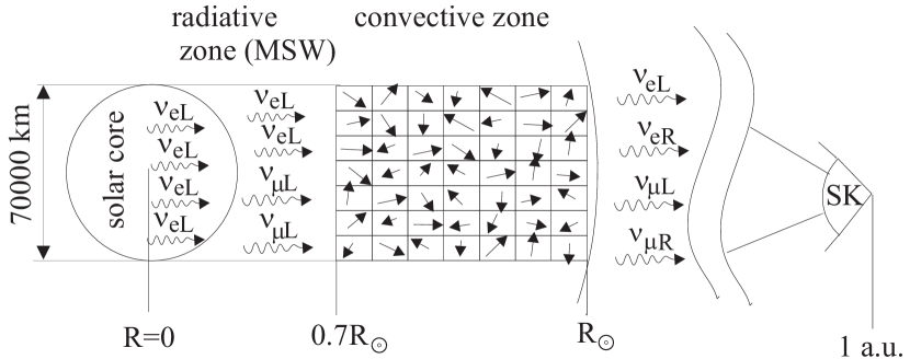
Figure 1: Geometry of neutrino trajectories in random magnetic fields. Finite radius of $\nu_{eL}$-neutrino source, the solar core radius $0.1R_{\odot}$, is shown.

the solar core with the radius of the order of $R_{\nu}=0.1R_{\odot}=7\times 10^{4}~{}km$. For the sake of simplicity we do not consider here the spatial distribution of neutrino emissivity from a unit of a solid angle of the core image and the differences in $R_{\nu}^{(i)}$ for different neutrino kinds ”i”. Different parallel trajectories directed to the Earth cross different magnetic domains because the domain size $L_{0}$ (in the plane which is perpendicular to neutrino trajectories) is much less than the transversal size $=R_{\nu}$ of the full set of parallel rays, $L_{0}\ll R_{\nu}$, see Fig. 1. The whole number of trajectories (rays) with statisticaly independent magnetic fields is about $R_{\nu}^{2}/L_{0}^{2}\sim 50$.

At the stage of numerical simulation of the random magnetic field we generate the set of random numbers with a given r.m.s. value and for each realization of random magnetic fields along each of $50$ rays solve the Cauchi problem for the $(4\times 4)$ master equation [2].

Then we calculate the dynamical probabilities $P_{aa}(t)$, and average them in transversal plane, i.e. obtain the mean arithmetic probabilities as functions of mixing parameters $\sin^{2}2\theta$ , $\delta$. We argue that being additive functions of the area of the convective zone layer (or, the same, of the number of rays) these probabilities with increasing area become self-averaged.

3 ASYMPTOTIC SOLUTION

To demonstrate the properties of our model we briefly discuss how random magnetic field influences the small-mixing MSW solution to SNP. It turns out that for the SSM exponential density profile, typical borone neutrino energies $E\sim 7\div 14MeV$, and $\triangle m^{2}\sim 10^{-5}~{}eV^{2}$, the MSW resonance occurs well below the bottom of the convective zone. Thus we can divide the neutrino propagation problem and consider two successive stages. First, after generation in the middle of the Sun, neutrinos propagate in the absence of any magnetic fields, undergo the non-adiabatic (non-complete) MSW conversion $\nu_{eL}\to\nu_{\mu L}$ and acquire certain nonzero values $P_{ee}$ end $P_{\mu\mu}$, which can be treated as initial conditions at the bottom of the convective zone. For small neutrino mixing $s_{2}\to 0$ the $(4\times 4)$-master equation [2] then splits into two pairs of independent equations describing correspondingly the spin-flavor dynamics $\nu_{eL}\to\tilde{\nu}_{\mu R}$ and $\nu_{\mu L}\to\tilde{\nu}_{eR}$ in noisy magnetic fields. In addition, once the MSW resonance point is far away from the convective zone, one can also omit $V_{e}$ and $V_{\mu}$ in comparison with $c_{2}\delta$. For $\nu_{eL}\to\tilde{\nu}_{\mu R}$ conversion this results into a two-component Schr$\rm\ddot{o}$dinger equation

$$i\left(\begin{array}[]{c}\dot{\nu}_{eL}\\ \dot{\tilde{\nu}}_{\mu R}\end{array}\right)\simeq\left(\begin{array}[]{cc}-\delta&\mu b_{+}(t)\\ \mu b_{-}(t)&\delta\end{array}\right)\left(\begin{array}[]{c}\nu_{eL}\\ \tilde{\nu}_{\mu R}\end{array}\right)$$ (4)

with initial conditions $|\nu_{eL}|^{2}(0)=P_{ee}(0),\quad|\tilde{\nu}_{\mu R}|^{2}=P_{\tilde{\mu}\tilde{\mu}}(0)=0.$ As normalized probabilities $P_{ee}(t)$ and $P_{\tilde{\mu}\tilde{\mu}}(t)$ (satisfying the conservation law $P_{ee}(t)+P_{\tilde{\mu}\tilde{\mu}}(t)=P_{ee}(0)$) are the only observables, it is convenient to recast Eq.(4) into an equivalent integral form

$$S(t)=S(0)-4\mu^{2}\int\limits_{0}^{t}dt_{1}\int\limits_{0}^{t_{1}}dt_{2}S(t_{2})\times$$

$$\times\{[b_{x}(t_{1})b_{x}(t_{2})+b_{y}(t_{1})b_{y}(t_{2})]\times$$

$$\times\cos 2\delta(t_{1}-t_{2})-[b_{x}(t_{1})b_{y}(t_{2})-$$

$$-b_{x}(t_{2})b_{y}(t_{1})]\sin 2\delta(t_{1}-t_{2})\},$$ (5)

where $S(t)=2P_{ee}(t)-P_{ee}(0)\equiv P_{ee}(t)-P_{\tilde{\mu}\tilde{\mu}}(t)$ is the third component of the polarization vector $\vec{S}$.

Let us trace the line of further derivation in a spirit of our numerical method. Dividing the interval of integration into a set of equal intervals of correlation length $L_{0},$ and assuming that possible correlations between $S(t_{2})$ and $b_{i},b_{j}$ under the integral are small, $S(t)$ itself varies very slowly within one correlation cell, and making use of statistical properties of random fields, ($i$) different transversal components within one cell are independent random variables, and ($ii$) magnetic fields in different cells do not correlate, we can average Eq.(5) thus obtaining a finite difference analogue. Returning back to continuous version we get

$$S(t)= S(0)\exp\Bigl{[}-\frac{4}{3}\mu^{2}L_{0}\frac{\sin^{2}\delta L_{0}}{(\delta L_{0})^{2}}\times$$ (6)

$$\times\int_{0}^{t}<\vec{b}^{2}(t^{\prime})>dt^{\prime}\Bigr{]}~{},$$

where we retained possible slow space dependence of the r.m.s. magnetic field value.

For $\delta~{}\ll L_{0}^{-1}$ and constant  r.m.s.  $<\vec{b}^{2}>$  we obtain the  simple  $\delta$-correlation  result [8] , [9], otherwise there remains an additional stabilizing factor $\sin^{2}x/x^{2}$, demonstrating to what extent the vacuum/medium neutrino oscillations within one correlation cell can suppress the spin-flavor dynamics due to the magnetic field only.

Another important issue is the problem of temporal dependence of higher statistical moments of $P_{aa}.$ As $P_{aa}$ enter the Eq.(1) for the number of events one should be certain that the averaging procedure does not input large statistical errors, otherwise there will be no room for the solar neutrino puzzle itself. For $\delta\ll L_{0}^{-1}$ basing on Eq. ( 5) we evaluate the dispersion $\sigma^{2}_{P}$. Here we present only the final result, the details of derivation will be published elsewhere:

$$\sigma_{P} = \sqrt{<P_{ee}^{2}(t)>-<P_{ee}(t)>^{2}}=$$ (7)

$$=\frac{P_{ee}(0)}{2\sqrt{2}}\left(1-e^{-2\Gamma t}\right)~{},$$

$$<P_{ee}(t)>=\frac{P_{ee}(0)}{2}\left(1+e^{-\Gamma t}\right),$$ (8)

where $\Gamma=(4/3)\mu^{2}<\vec{b}^{2}>L_{0}$. We see that relative mean square deviation of $P_{ee}$ from its mean value tends with $t\to\infty$ to its maximum asymptotic value

$$\frac{\sigma_{P}(t)}{<P_{ee}(t)>}\to\frac{1}{\sqrt{2}}\simeq 0.707,\qquad t\to\infty,$$ (9)

irrespectively of the initial value $P_{ee}(0).$

This estimate is true, evidently, only for one neutrino ray. Averaging over $N$ independent rays lowers the value (9) in $\sqrt{N}$ times. That is for our case of $N\approx 50$ rays we get that maximum relative error should not exceed approximately $10\%,$ thus justifying the validity of our approach. For smaller magnetic fields the situation is always better.

To conclude this section, it is neccesary to repeat that the above estimate Eq. (9) indicates possible danger when treating numerically the neutrino propagation in noisy media. Indeed, usually adopted one-dimensional (i.e. along one ray only) approximation for the $(4\times 4)$ master equation [2] or $(2\times 2)$ Eq. (4) can suffer from large dispersion errors and one should make certain precautions when averaging these equations over the random noise before numerical simulations. Otherwise, the resulting error might be even unpredictable.

4 DISCUSSION and CONCLUSIONS

In order to find the regions in the $\Delta m^{2}$, $\sin^{2}2\theta$ plane excluded from nonobservation of $\bar{\nu}_{eR}$ in SK it is necessary to compute and plot the isolines of the ratio $\Phi_{\bar{\nu}}/\Phi_{B}^{SSM}$. Indeed, as antineutrinos were not detected in the SK experiment one should claim that antineutrino flux is smaller than the SK background $\Phi_{\bar{\nu}_{e}}(E>8.3~{}MeV)<6\times 10^{4}~{}cm^{-2}s^{-1}$  [3]. Deviding this inequality by the SSM borone neutrino flux with energies $E>E_{th}=8.3~{}MeV$,   $\Phi_{B}^{SSM}(E>8.3~{}MeV)=1.7\times 10^{6}~{}cm^{-2}s^{-1}$ we find the bound on the averaged over cross-section and spectrum, cascade transition probability $\nu_{eL}\to\bar{\nu}_{eR}$ ,

$$\frac{\Phi_{\bar{\nu}_{e}}(E>8.3~{}MeV)}{\Phi_{B}^{SSM}(E>8.3)}=$$

$$=\frac{\int_{8.3}^{15}\lambda_{B}(E)P_{\bar{e}\bar{e}}(E)\sigma_{\bar{\nu}}(E)dE}{\int_{8.3}^{15}\lambda_{B}(E)\sigma_{\bar{\nu}}(E)dE}\leq 0.035~{},$$ (10)

or $\Phi_{\bar{\nu}}/\Phi_{B}^{SSM}\leq 3.5$% . Here $\sigma_{\bar{\nu}}(E)=9.2\times 10^{-42}~{}cm^{2}[(E-1.3~{}MeV)/10~{}MeV]^{2}$ is the cross-section of the capture reaction $\bar{\nu}_{e}p\to ne^{+}$. Notice that the above bound is not valid for low energy region below the threshold of the antineutrino capture by protons, $E\leq 1.8~{}MeV$.

For low magnetic fields, $B~{},b\leq 20~{}kG$, both for regular and random ones we do not find any violation of the bound Eq. (10). However, for strong magnetic fields such forbidden parameter regions appear in different areas over $\delta$ and $\sin^{2}2\theta$ for different kind of magnetic fields (regular and random). In general, the influence of random magnetic fields is more pronounced as compare to the regular ones of the same strength.

This property of random fields was illustrated in our work [2] both for regular and random magnetic fields.

It follows that the more intensive the r.m.s. field $\sqrt{\langle b^{2}\rangle}$ in the convective zone the more effective spin-flavour conversions lead to the production of the right-handed $\bar{\nu}_{eR}$, $\bar{\nu}_{\mu R}$-antineutrinos. In the case of small mixing this is also seen from Eq. (6).

Our results, however, show that there exists strong dependence not only on the r.m.s. magnetic field strength but on its correlation length also. In particular, when for the same $b_{rms}=100~{}kG$ we substitute $L_{0}=10^{3}~{}km$ (a granule size) instead of $L_{0}=10^{4}~{}km$ (a mesogranule size treated in numerical simulation) the small mixing MSW region is fully excluded via the SK bound Eq. (10) (see Fig. 14 in [2]). This is easily explained due to the maximum value of ASFC seen from Eq. (6) ($\sin x/x\to 1$). Vice versa, if the small-mixing MSW solution is valid and a large neutrino magnetic moment exists we can extract from neutrino data important constraints on the structure of random magnetic fields deep under surface of the Sun.

Extrapolating the tendency above either with a decrease of the correlation length $L_{0}\leq 10^{3}~{}km$ or with an increase of the magnetic field values $b_{r.m.s.}\geq 100~{}kG$ (or for both changes) we could also exclude LMA MSW region or both standard MSW regions would be forbidden.

However, for such case one finds LOW MSW with $\Delta m^{2}\sim 10^{-7}~{}eV^{2}$, $\sin^{2}2\theta\sim 0.8$ becomes to be allowed being forbidden for larger correlation lengths ($L_{0}\geq 10^{4}~{}km$) and lower r.m.s. values ($b\leq 100~{}kG$) (see Fig. 14 in [2]).

Thus, we develop a model of neutrino spin-flavour conversions in the random magnetic fields of the solar convective zone supposing in consistence with modern MHD models of solar magnetic fields that random fields are naturally much higher than large-scale magnetic fields  created and supported  continuously from the small-scale  random ones [6].

It follows that if neutrinos have a large transition magnetic moment their dynamics in the Sun is governed by random magnetic fields that , first, lead to aperiodic and rather non-resonant neutrino spin-flavor conversions, and second, inevitably lead to production of electron antineutrinos for low energy or large mass difference region.

Analogous results were obtained in the work [11] where the averaging of the Redfield equation for the $4\times 4$ density matrix over $\delta$-correlated random magnetic fields allowed to get simple asymptotical solutions for strong random fields and led to the same aperiodic form of the probabilities as in Eq.(8).

However, for the realistic case of solar random magnetic fields with a finite correlation length the method of direct numerical simulation of the Schroedinger equation given in [2] is more appropriate. Then the averaging of numerical solutions (not Schroedinger equation!) over an ensemble of random field configurations (see Fig. 1) gives correct results for this case.

If antineutrinos $\bar{\nu}_{eR}$ would be found with the positive signal in the BOREXINO experiment[12] or, in other words, a small-mixing MSW solution to SNP fails, this will be a strong argument in favour of magnetic field scenario with ASFC in the presence of a large neutrino transition moment, $\mu\sim 10^{-11}\mu_{B}$ for the same small mixing angle.

The search of bounds on $\mu$ at the level $\mu\sim 10^{-11}\mu_{B}$ in low energy $\nu~{}e$-scattering, currently planning in laboratory experiments [13], will be crucial for the model considered here.

We would like to emphasize the importance of future low-energy neutrino experiments (BOREXINO, HELLAZ) which will be sensitive both to check the MSW scenario and the $\bar{\nu}_{eR}$-production through ASFP. As it was shown in a recent work[14] a different slope of energy spectrum profiles for different scenarios would be a crucial test in favour of the very mechanism providing the solution to SNP.

References

-
[1]
The Super-Kamiokande collaboration, Phys. Rev. Lett. 82 (1999) 2430;
hep-ex/9812011 - [2] A.A. Bykov, V.Yu. Popov, A.I. Rez, V.B. Semikoz and D.D. Sokoloff, Phys. Rev. D 59 (1999) 063001.
- [3] G. Fiorentini, M. Moretti and F.L. Villante, Phys. Lett. B413 (1997) 378; hep-ph/9707097
- [4] E.Kh. Akhmedov, A. Lanza, S.T. Petcov, Phys. Lett. B348 (1995) 124.
- [5] A.A. Bykov, V.Yu. Popov, T.I. Rashba and V.B. Semikoz (in preparation)
-
[6]
E. N. Parker, Astrophys. J. 408 (1993) 707;
E. N. Parker, Cosmological Magnetic Fields (Oxford University Press, Oxford, 1979). - [7] S. I. Vainstein, A. M. Bykov, I. M. Toptygin, Turbulence, Current Sheets and Shocks in Cosmic Plasma (Gordon and Breach, 1993).
- [8] A. Nicolaidis, Phys.Lett. B262 (1991) 303.
- [9] K. Enqvist, A. I. Rez, V. B. Semikoz, Nucl. Phys. B436 (1995) 49.
- [10] E .Kh. Akhmedov, The neutrino magnetic moment and time variations of the solar neutrino flux , Preprint IC/97/49. Invited talk given at the 4-th International Solar Neutrino Conference (Heidelberg, Germany, April 8-11, 1997).
- [11] V.B. Semikoz, E. Torrente-Lujan, hep-ph/9809376, to appear in Nucl. Phys. B.
- [12] J. B. Benziger et al., Status Report of Borexino Project: The Counting Test Facility and its Results. A proposal for participation in the Borexino Solar Neutrino Experiment (Princeton, October 1996). Talk presented by T.E. Hagner at X Baksan International School “Particles and Cosmology ” (April 1999).
- [13] I. R. Barabanov et al., Astroparticle Phys. 5 (1996) 159.
-
[14]
S. Pastor, V.B. Semikoz, and
J.W.F. Valle, Phys.Lett. B423 (1998) 118.