THU-99-16
ITFA-99-16
hep-ph/9906538
June 1999

Particle Production and Effective Thermalization
in
Inhomogeneous Mean Field Theory

Abstract

As a toy model for dynamics in nonequilibrium quantum field theory we consider the abelian Higgs model in $1+1$ dimensions with fermions. In the approximate dynamical equations, inhomogeneous classical (mean) Bose fields are coupled to quantized fermion fields, which are treated with a mode function expansion. The effective equations of motion imply e.g. Coulomb scattering, due to the inhomogeneous gauge field. The equations are solved numerically. We define time dependent fermion particle numbers with the help of the single-time Wigner function and study particle production starting from inhomogeneous initial conditions. The particle numbers are compared with the Fermi-Dirac distribution parametrized by a time dependent temperature and chemical potential. We find that the fermions approximately thermalize locally in time.

1 Introduction

One issue that is of considerable interest in nonequilibrium quantum field theory is equilibration and thermalization. An understanding of this is crucial for the knowledge of e.g. the rate at which a quark-gluon plasma forms in heavy ion collisions, or the rate at which a Bose gas thermalizes locally in time during evaporative cooling. In cosmology, the study of (pre)heating of the universe at the end of inflation has become a topic of its own.

Real time evolution of quantum fields can in general not be solved exactly. A popular approach in nonequilibrium field theory is then to use large $N$ or Hartree-like approximations, in which coupled equations for mean fields and their fluctuations are solved self-consistently [1, 2, 3, 4, 5, 6, 7]. In many treatments available in the literature, the mean fields are taken to be homogeneous. Thermalization may be difficult to achieve in these approximations [2, 3, 4, 5, 6] (see in this respect also [8]). Another approach is to treat the dynamics of the low momentum modes classically [9, 10].

In this paper we study numerically the real time dynamics in the abelian Higgs model in $1+1$ dimensions, extended with fermions. The choice of model is motivated by electroweak baryogenesis [11], e.g. according to the scenario in ref. [12]. We use a large $N$ approximation in which the Bose fields are treated as mean fields and the fermion fields play the role of fluctuations. Previous numerical studies of fermions in real time have been restricted to homogeneous mean fields, with [5, 6] or without [13] back reaction. Instead, in our case the mean fields are inhomogeneous and they obey the full non-linear classical field equations including the back reaction of the fermions. This back reaction is represented by mode functions which obey the Dirac equation in the presence of the mean fields. Loosely speaking, the effective equations describe a collection of quantum mechanical particles (the fermion modes) coupled to classical fields (the mean fields). The particles therefore interact and scatter amongst themselves as in classical electrodynamics. In particular Coulomb forces, screened by the Higgs field, are expected to play an important role.

We focus on the following dynamical problem: initially, all the energy is contained in a few long wave lengths of the Bose fields, and the fermions are in a vacuum state. This is a nonequilibrium situation and in course of time energy is transferred towards the fermionic degrees of freedom, producing fermion particles. A motivation is partly given by inflation, where at the end of inflation the energy stored in the inflaton field is transferred to other degrees of freedom, leading to the (pre)heating of the universe (see e.g. [3, 6, 13, 14]).

In the presence of spacetime dependent mean fields the identification of particles is usually based on the concept of adiabatic particle numbers [2, 3, 4, 5, 6]. If the model can be described in terms of weakly coupled quasiparticles, it should also be possible to deduce a particle number directly from correlation functions. In a gauge theory, simple correlation functions such as the fermion two-point function are not gauge invariant and the calculation would have to be performed in a fixed gauge. This introduces an ambiguity whether the resulting particle number depends on the gauge. However, physical observables calculated in terms of these particle numbers should come out gauge independent. Another possibility is to use a gauge invariant modification of the two-point function. There are several ways in which this can be done and a simple one is by including a parallel transporter between the two fermion fields at different points in space. This gives a close connection to the Wigner function.

The Wigner function has a long history in transport theory and quantum kinetic theory [15]. It has been used to find approximative ways to deal with dynamical issues in out-of-equilibrium plasmas. Recently, the Wigner function has been used quite extensively to derive transport equations that contain the same physics as the Hard Thermal Loops in $3+1$ dimensional gauge plasmas [16]. A comparison between so-called covariant and single-time formulations is given in [17]. In this paper we use the single-time Wigner function, not for dealing with the dynamics but merely as a tool for identifying the particle number. We solve the microscopic dynamics numerically in the large $N$ approximation and then calculate the single-time Wigner function. After averaging over space and a short interval in time to smoothen the effect of oscillating Bose fields, we extract the particle number by comparing the Wigner function with that of a free fermion gas. This approach is obviously only valid when the theory is relatively weakly coupled and a description in terms of quasiparticles makes sense.

The paper is organized as follows. In section 2 we introduce the model and give the effective equations of motion. A discussion of the particle number from the fermion two-point function and the Wigner function is given in section 3. In section 4, we present numerical results for the real time evolution and the time dependent particle number, starting from a nonequilibrium initial state. To see whether the particles are effectively thermalized, we compare the particle numbers with the Fermi-Dirac distribution depending on time dependent temperature and chemical potential. The results are summarized in the Conclusion. The equations are solved numerically on a lattice in space and time. Some aspects of the lattice implementation are briefly described in appendix A. Details relating the Wigner function and the gauge fixed two-point function are given in appendix B.

We refer to our previous paper [7] for more details on the model, the effective equations of motion, and a discussion of the lattice implementation.

2 Action and mean field equations of motion

We consider the abelian Higgs model in $1+1$ dimensions, with $n_{f}=2$ flavours of fermions. The action reads

$$S\!\!\! = \!\!\!-\int d^{2}x\Bigg{[}\frac{1}{4e^{2}}F_{\mu\nu}F^{\mu\nu}+(D_{\mu}\phi)^{*}D^{\mu}\phi+\lambda\left(\phi^{*}\phi-v^{2}/2\right)^{2}$$

$$\;\;\;\;\;\;\;+\bar{\psi}_{i}\gamma^{\mu}(\partial_{\mu}-iqA_{\mu})\psi_{i}+\frac{1}{2}\sum_{i}(G_{i}\psi_{i}^{T}{\cal C}^{\dagger}\phi^{*}\psi_{i}-G_{i}\bar{\psi}_{i}{\cal C}\phi\bar{\psi}_{i}^{T})\Bigg{]}.$$

Here $F_{\mu\nu}=\partial_{\mu}A_{\nu}-\partial_{\nu}A_{\mu}$, $D_{\mu}=\partial_{\mu}-iA_{\mu}$, ${\cal C}$ denotes the charge conjugation matrix and $\bar{\psi}=\psi^{\dagger}\beta$. An explicit representation for the gamma-matrices is $\gamma^{1}=\sigma_{1},{\cal C}=\beta=i\gamma^{0}=\sigma_{2}$, and $\gamma_{5}=-\gamma^{0}\gamma^{1}=\sigma_{3}$. Space is a circle with circumference $L$ and the Bose (fermion) fields obey (anti)periodic boundary conditions. Other conventions can be found in [7]. The choice of this model, in particular the form of the Yukawa coupling, is motivated by electroweak baryogenesis, but we will not elaborate on those aspects here (see instead [7]). The fermion field carries a flavour index $i=1,2=n_{f}$ and the Yukawa coupling $G_{i}$ depends on the flavour: $G_{1}=-G_{2}\equiv G$. Local gauge symmetry acts as $\phi\to e^{i\xi}\phi,\psi_{i}\to e^{iq\xi}\psi_{i},A_{\mu}\to A_{\mu}+\partial_{\mu}\xi$, with $q=\frac{1}{2}$, so that the Yukawa term is gauge invariant. In this paper we restrict ourselves, however, to massless fermions and put the Yukawa term to zero, $G=0$.

The global symmetry $\psi_{i}\to e^{i\omega\gamma_{5}}\psi_{i}$ is broken in the quantum theory due to the axial anomaly, and

$$\partial_{\mu}j_{5}^{\mu}=n_{f}\frac{1}{4\pi}\epsilon^{\mu\nu}F_{\mu\nu}=n_{f}\partial_{\mu}C^{\mu},$$

with the axial current $j_{5}^{\mu}=i\bar{\psi}_{i}\gamma^{\mu}\gamma_{5}\psi_{i}$ and the Chern-Simons current $C^{\mu}=\epsilon^{\mu\nu}A_{\nu}/2\pi$. A change in the axial charge is proportional to a change in the Chern-Simons number

$$Q_{5}(t)-Q_{5}(0)=n_{f}(C(t)-C(0)),$$ (2.1)

with $Q_{5}(t)=\int dx\,j^{0}_{5}(x,t)$, and $C(t)=-(2\pi)^{-1}\int dx\,A_{1}(x,t)$. As in the electroweak theory, integer values of the Chern-Simons number label the non-trivial vacua of the bosonic theory. The $q=\frac{1}{2}$ charged fermions change the periodicity of the classical bosonic ground state: only vacua with Chern-Simons numbers that differ an even integer (instead of any integer) are connected by large gauge transformations. The vacua are separated by finite energy barriers, the sphaleron configuration at half integer $C$.

As an approximation to solve the dynamics, we treat the Bose fields as mean fields and the fermion fields as fluctuations. A formal derivation can be given by duplicating the fermion fields $N$ times and taking the large $N$ limit, after a proper rescaling of the coupling constants and fields [1, 7]. The resulting equations are (in the $A_{0}=0$ gauge)

$$\partial^{2}_{0}A_{1}(x,t)\!\!\! = \!\!\!e^{2}\left[j_{h}^{1}(x,t)+\langle j_{f}^{1}(x,t)\rangle\right],$$ (2.2)

$$\partial_{0}^{2}\phi(x,t)\!\!\! = \!\!\!D^{2}_{1}\phi(x,t)-2\lambda\left[|\phi(x,t)|^{2}-v^{2}/2\right]\phi(x,t),$$ (2.3)

together with Gauss’ law

$$\partial_{1}\partial_{0}A_{1}(x,t)=-e^{2}\left[j_{h}^{0}(x,t)+\langle j_{f}^{0}(x,t)\rangle\right].$$ (2.4)

The scalar contribution to the current, $j^{\mu}_{h}$, is given by

$$j^{\mu}_{h}(x,t)=i(D^{\mu}\phi(x,t))^{*}\phi(x,t)-i\phi^{*}(x,t)D^{\mu}\phi(x,t).$$ (2.5)

The fields $A_{1}$ and $\phi$ represent mean fields, which can be inhomogeneous in general,

$$A_{1}(x,t)\equiv\langle A_{1}(x,t)\rangle,\;\;\;\;\phi(x,t)\equiv\langle\phi(x,t)\rangle.$$

The fermion contribution to the current is

$$j^{\mu}_{f}(x,t)=\frac{q}{2}i[\bar{\psi}_{i}(x,t),\gamma^{\mu}\psi_{i}(x,t)],$$

and its expectation value represents the fermion back reaction. The commutator ensures that the current is odd under charge conjugation.

The most demanding part of this approach is the calculation of the back reaction. In the case of homogeneous mean fields, the usual manner is to use a mode function expansion. We use the same method in the inhomogeneous case as well.

The back reaction is calculated by expanding the fermion fields in a complete set of eigenspinors of the initial Dirac hamiltonian at $t=0$. This leads to a mode function expansion,

$$\psi_{i}(x,t)=\sum_{p}\left[b_{pi}u_{pi}(x,t)+d^{\dagger}_{pi}v_{pi}(x,t)\right].$$ (2.6)

The coefficients $b^{(\dagger)}_{pi},d^{(\dagger)}_{pi}$ are time independent and represent the annihilation (creation) operators of particles resp. antiparticles at the initial time. They obey the usual anticommutation relations

$$\{b^{\dagger}_{pi},b_{p^{\prime}i^{\prime}}\}=\delta_{pp^{\prime}}\delta_{ii^{\prime}},\;\;\;\;\{d^{\dagger}_{pi},d_{p^{\prime}i^{\prime}}\}=\delta_{pp^{\prime}}\delta_{ii^{\prime}},$$

and zero for others. The expectation values of the creation and annihilation operators in (2.6) determines the initial state for the fermions. We take vacuum initial conditions for the fermions, so that the only non-zero expectation values are

$$\langle b_{pi}b^{\dagger}_{pi}\rangle=\langle d_{pi}d^{\dagger}_{pi}\rangle=1.$$ (2.7)

The fermion contribution to the current can now be expressed in terms of the mode functions,

$$\langle j^{\mu}_{f}(x,t)\rangle=-\sum_{p}\frac{q}{2}\left[\bar{u}_{pi}(x,t)i\gamma^{\mu}u_{pi}(x,t)-\bar{v}_{pi}(x,t)i\gamma^{\mu}v_{pi}(x,t)\right].$$ (2.8)

The time dependence is carried by the spinor mode functions $u$ and $v$, which are solutions of the Dirac equation in the presence of the gauge field,

$$i\partial_{0}u_{pi}(x,t)={{\cal H}_{D}}[A_{1}(x,t)]u_{pi}(x,t),$$ (2.9)

and similar for $v_{pi}$. The Dirac hamiltonian has the usual form

$${{\cal H}_{D}}=-i\alpha^{1}(\partial_{1}-iqA_{1}),\;\;\;\;\alpha^{1}=-\gamma^{0}\gamma^{1}.$$ (2.10)

The initial conditions for the mode functions are given by

$$u_{pi}(x,0)=\frac{1}{\sqrt{L}}e^{ipx}u_{pi},\;\;\;\;v_{pi}(x,0)=\frac{1}{\sqrt{L}}e^{-ipx}v_{pi},$$

with $u_{pi}(v_{pi})$ positive (negative) energy spinors of the Dirac hamiltonian at $t=0$: $p$ labels the momentum eigenstates of the initial Dirac hamiltonian. It takes the values

$$p=\frac{2\pi}{L}(n-\frac{1}{2}),$$

due to the antiperiodic boundary conditions on the fermion fields. For these initial conditions with vacuum expectation values (2.7), the current (2.8) vanishes at $t=0$.

If the mean fields are restricted to be homogeneous, plane waves $e^{\pm ipx}$ multiplying the mode functions can be factored out at all times, and each mode function is the solution of an ordinary differential equation. In the more general case that the mean fields are allowed to be inhomogeneous, this is not possible, and a large set of partial differential equations has to be solved. In that case the label $p$ looses its interpretation for $t>0$, and it simply labels a complete set.

The equations of motion are free from ultraviolet divergences and the sum over the mode functions in (2.8) is finite. In the higher dimensional case charge renormalization would be necessary [1]. For a study of renormalization in the presence of the Yukawa term we refer to our previous paper [7]. The energy of the system is the sum of the energy in the Bose fields and the fermion fields. The energy of the fermions at time $t$ is given by the expectation value $E_{F}(t)=\sum_{x}\langle\psi_{i}^{\dagger}(x,t){{\cal H}_{D}}\psi_{i}(x,t)\rangle$ and can be expressed as a sum over mode functions. This sum is quadratically divergent. In the numerical implementation this is regulated by the lattice cutoff: the effective equations are solved using a discretization on a lattice in space and real time (see appendix A). We renormalize the energy by subtracting the bare fermion energy at $t=0$.

3 Particle number and the Wigner function

Observables which may give insight about what happens on the microscopic level during time evolution are current, charge and energy densities. These are gauge invariant quantities whose physical meaning is clear and unambiguous and they are straightforward to calculate. In addition to this, it has been shown in the case of homogeneous mean fields that more insight can be found with the concept of adiabatic or instantaneous particle number.

The adiabatic particle number is based on an expansion of the (interacting) quantum field at each instant in time in terms of a complete set of eigenfunctions of the Dirac hamiltonian at time $t$ (we suppress flavour indices here)

$$\psi(x,t)=\sum_{E}\left[\tilde{b}_{E}(t)\tilde{u}_{E}(x,t)+\tilde{d}_{E}^{\dagger}(t)\tilde{v}_{E}(x,t)\right].$$ (3.1)

The coefficients of these eigenfunctions are then identified with time dependent creation and annihilation operators. In (3.1) the eigenfunctions are denoted with $\tilde{u}_{E},\tilde{v}_{E}$, and the complete set is labeled with $E$. A Bogoliubov transformation relates the expansions (2.6) and (3.1). The instantaneous particle numbers at time $t$ are then defined by the expectation values

$$N_{E}(t)=\langle\tilde{b}^{\dagger}_{E}(t)\tilde{b}_{E}(t)\rangle,\;\;\;\;\bar{N}_{E}(t)=\langle\tilde{d}^{\dagger}_{E}(t)\tilde{d}_{E}(t)\rangle.$$

In the case of homogeneous mean fields the instantaneous eigenfunctions can be calculated analytically, in terms of plane waves. For the inhomogeneous case the diagonalization will in general have to be performed numerically, which makes the calculation rather involved. Furthermore, the instantaneous eigenmodes of the Dirac hamiltonian are not easily interpreted in terms of familiar concepts like quasiparticles, e.g. concerning the relation between $E$ and the quasiparticle momentum. Therefore we now discuss another approach, using correlation functions.

The identification of particles can be motivated in general (for a weakly coupled system) by comparison with the noninteracting case, and for free fields the two-point function provides all the available information. Fields in equilibrium are homogeneous in space and time. In the interacting situation, one can look for subsets of the system which are effectively in equilibrium. Such subsets will only exist locally in space and time, and one way to enforce homogeneity is averaging over small subset-volumes of spacetime. This then leads to a definition of particle numbers locally in space and time. The optimal size of the subsets is not known a priori, and this may introduce a certain ambiguity. The dependence on the size of the subsets can be studied by changing it.

One way to implement this idea is by studying the equal-time two-point function

$$S(x,y;t)=\langle\psi(x,t)\bar{\psi}(y,t)\rangle,$$ (3.2)

in particular in the following manner

$$S_{\rm av}(p,t)=\frac{1}{t_{\rm av}}\int_{t-t_{\rm av}/2}^{t+t_{\rm av}/2}dt^{\prime}\,S(p,t^{\prime}),\;\;\;\;S(p,t)=\int dz\,e^{-ipz}\frac{1}{L}\int dx\,S(x,x+z;t).$$ (3.3)

The time average over a short time interval $t_{\rm av}$ will smoothen oscillations in the Bose fields, and instead of averaging over smaller spatial subsets, we choose here to integrate over the complete spatial volume. Hence, the particle numbers will be defined locally in time only. This simplifies the analysis and has the positive effect of diminishing the fluctuations. As a side remark, it can be checked explicitly that this approach reduces to a commonly used definition of particle number for the case of homogeneous mean fields [5, 6].

The fermion correlator is not gauge invariant, but the concept of quasiparticles is not gauge invariant in the first place, although using them to compute observables such as energy and pressure should give gauge invariant answers. Therefore, before averaging over space and time we need to fix the gauge. A suitable choice is the temporal Coulomb gauge, $A_{0}=0$, $\partial_{1}A_{1}=0$, in which the remaining freedom of ‘large’ gauge transformations is removed by requiring $C=-LA_{1}/(2\pi)\in(-1,1]$.

There are of course other possibilities. One is to use gauge invariant modifications of the fermion correlator (3.2), for example,

$$W(x,y;t)=\langle\psi(x,t)\bar{\psi}(y,t)U(y,x;t)\rangle,$$ (3.4)

where $U$ is the parallel transporter

$$U(y,x;t)=\exp\left[-iq\int_{y}^{x}ds\,A_{1}(s,t)\right].$$

The path is along the shortest straight line connecting $x$ and $y$. Other paths are possible as well, which leads to a class of gauge invariant modifications of the two-point function (3.2). The arbitrariness in choosing a gauge is now replaced by choosing a gauge invariant correlator. The above $W(x,y;t)$ is closely related to the single-time Wigner function [15, 17]. In terms of the relative coordinate $z=x-y$ and the center-of-mass coordinate $X=\frac{1}{2}(x+y)$, the single-time Wigner function is given by a spatial Fourier transform of (3.4) with respect to $z$,

$$W(X,p;t)=\int dz\,e^{-ipz}\,W(X+\frac{1}{2}z,X-\frac{1}{2}z;t).$$

We shall use its spatial and temporal average,

$$W_{\rm av}(p,t)=\frac{1}{t_{\rm av}}\int_{t-t_{\rm av}/2}^{t+t_{\rm av}/2}dt^{\prime}\,W(p,t^{\prime}),\;\;\;\;W(p,t)=\frac{1}{L}\int dX\,W(X,p;t),$$ (3.5)

similar as for the two-point function, (3.3). In appendix B we show that the correlators $S(p,t)$ and $W(p,t)$ are actually closely related by mere interpolation between the discrete momenta $p$. In the following we shall continue with the Wigner function.

In the spinor decomposition (in $1+1$ dimensions), four functions appear

$$W(X,p;t)={\cal F}(X,p;t)+i\gamma^{\mu}{\cal V}_{\mu}(X,p;t)+i\gamma_{5}{\cal P}(X,p;t),$$ (3.6)

that are real, due to the elementary property $W^{\dagger}(X,p;t)=\beta W(X,p;t)\beta$. We shall use the obvious notation ${\cal F}_{\rm av}(p,t)$, etc., for temporally and spatially averaged coefficients.

For fermions characterized by momentum $p$ and mass $m$, the free field expression for the Wigner function is given by

$$W_{\rm free}(X,p)\!\!\! = \!\!\!(1-N_{p}-\bar{N}_{-p})\frac{m-i\gamma^{1}p}{2E_{p}}+\frac{1}{2}i\gamma^{0}(1-N_{p}+\bar{N}_{-p}),$$ (3.7)

$$E_{p}\!\!\! = \!\!\!\sqrt{m^{2}+p^{2}}.$$

The arbitrary (anti)particle occupation numbers are given by $N_{p}$ ($\bar{N}_{p}$). Since this is independent of $X$, we now take as a possible definition of time dependent particle numbers $N_{p}(t)$, $\bar{N}_{p}(t)$ and effective mass $m_{p}(t)$, the solution of the three equations

$${\cal F}_{\rm av}(p,t)\!\!\! = \!\!\!\frac{1}{2}\mbox{Tr}\,W_{\rm av}(p,t)=\frac{1}{2}\left[1-N_{p}(t)-\bar{N}_{-p}(t)\right]\frac{m_{p}(t)}{\sqrt{m_{p}^{2}(t)+p^{2}}},$$ (3.8)

$$-{\cal V}_{1{\rm av}}(p,t)\!\!\! = \!\!\!\frac{1}{2}\mbox{Tr}\,i\gamma^{1}W_{{\rm av}}(p,t)=\frac{1}{2}\left[1-N_{p}(t)-\bar{N}_{-p}(t)\right]\frac{p}{\sqrt{m_{p}^{2}(t)+p^{2}}},$$ (3.9)

$${\cal V}_{0{\rm av}}(p,t)\!\!\! = \!\!\!\frac{1}{2}\mbox{Tr}\,i\gamma^{0}W_{{\rm av}}(p,t)=\frac{1}{2}\left[1-N_{p}(t)+\bar{N}_{-p}(t)\right].$$ (3.10)

The explicit solution of these equations is given in appendix B. We have added a subscript $p$ on the effective mass parameter to indicate a possible momentum dependence. The interpretation of $m_{p}$ as a mass is of course best when $m_{p}(t)$ is momentum independent, as in the free field case. A comparison with free Wigner function (3.7) gives zero for the fourth function ${\cal P}_{\rm av}(p,t)=-\mbox{Tr}\,i\gamma_{5}W_{{\rm av}}(p,t)$. Hence, this coefficient cannot be used to find new information on the particle numbers or effective mass, but it serves as a consistency check.

Note that when the mean fields are homogeneous, particles and antiparticles with momentum $p$ can only be produced in pairs, and $N_{p}=\bar{N}_{-p}$. In general, they can be different. It should be clear that we use the Wigner function only to identify the instantaneous particle number at time $t$ (i.e. after averaging over the short interval $t_{\rm av}$). Therefore we consider the single-time Wigner function instead of the covariant one. We do not attempt to solve the dynamics using the Wigner function approach.

Our goal is now to solve the effective equations for the Bose fields and the spinor mode functions. The Wigner function can be expressed in terms of the mode functions using the expansion (2.6), and from a calculation of ${\cal F}_{\rm av}(p,t)$, ${\cal V}_{\mu{\rm av}}(p,t)$ and ${\cal P}_{\rm av}(p,t)$ the particle number can be extracted. This will be the subject of the following section.

4 Particle production

We solve the closed set of effective equations (2.2–2.5, 2.8–2.10) numerically. In this paper we take the following parameters: the dimensionful parameters are related by $\lambda/e^{2}=0.25,eL=3.2$ and the dimensionless parameter in the scalar potential is $v^{2}=8$. Then the volume is not very large but also not too small: in terms of the tree level boson masses, $m_{\phi}L=\sqrt{2\lambda}vL\approx 6.4$, $m_{A}L=evL\approx 9.1$. Furthermore, the couplings are fairly weak: $e^{2}/m^{2}_{\phi}=0.25$. Some details on the lattice implementation and choice of parameters can be found in appendix A.

The inhomogeneous Bose fields are initialized such that all the energy initially resides in the long wave lengths. We take vacuum field configurations $\phi(x,0)=v/\sqrt{2}$, $A_{1}(x,0)=0$, and use space dependent momenta. The results presented below are obtained starting with

$$\partial_{0}\phi(x,0)=3e\cos\frac{2\pi x}{L}+2ie\cos\frac{2\pi x}{L},\;\;\;\;\partial_{0}A_{1}(x,0)=\mbox{Gauss' law}+e^{2}.$$

The electric field $\partial_{0}A_{1}(x,0)$ is determined almost completely by the Gauss law (2.4), up to a constant.

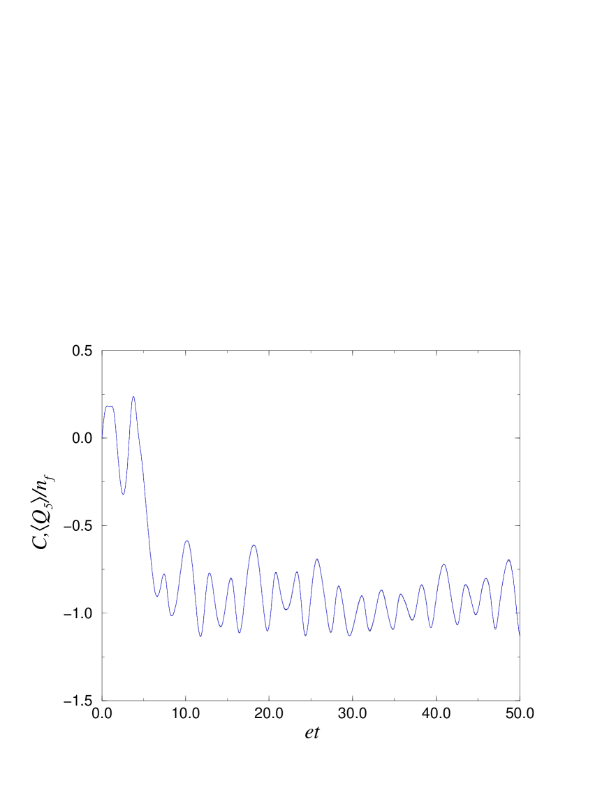
Figure 1: Chern-Simons number $C$ and axial charge per flavour $\langle Q_{5}\rangle/n_{f}$ versus $et$. The lines fall on top of each other, as expected from the anomaly equation.

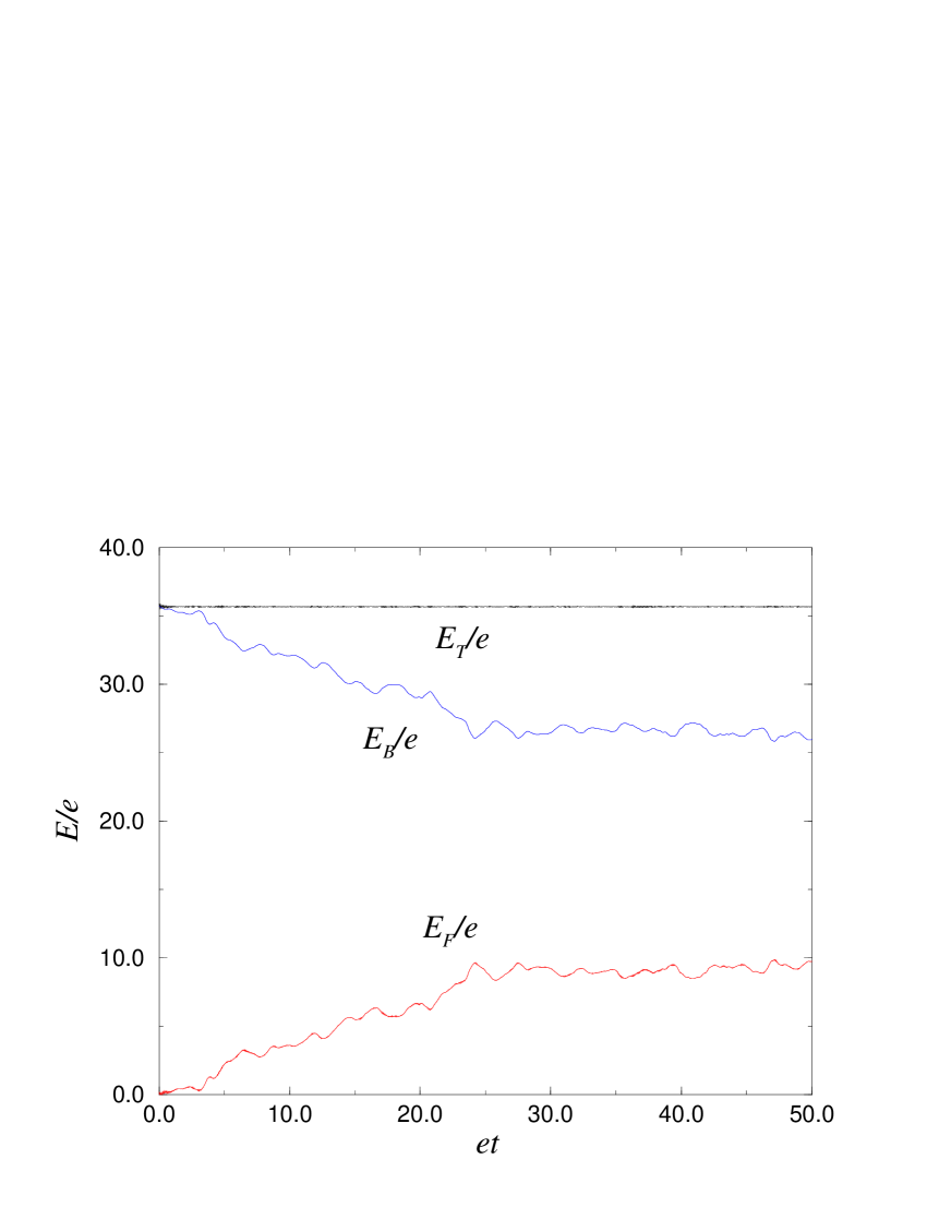
Figure 2: Energy in units of $e$ in the Bose fields ($E_{B}$), fermion fields ($E_{F}$) and their conserved sum $E_{T}$ versus $et$.

The Chern-Simons number $C$ and the axial charge per flavour $\langle Q_{5}\rangle/n_{f}$, which agree in accordance with the anomaly equation (2.1), are shown during time evolution in fig. 1. Time is given in units of $1/e$, which has the dimension of mass in $1+1$ dimensions. We see one sphaleron transition. The energy of the Bose fields, the fermion fields and the total conserved energy are shown in fig. 2. Initially, the (renormalized) fermion energy is zero, because of the vacuum initial conditions for the fermions. We see that there is energy transfer towards the fermion degrees of freedom.

To analyse how the energy is distributed in the fermion subsystem we have calculated the four functions ${\cal F}(p,t),{\cal V}_{\mu}(p,t)$ and ${\cal P}(p,t)$ which appear in the spinor decomposition of the Wigner function (3.5, 3.6), and averaged them over a relatively short time interval $et_{\rm av}=4$. This interval is comparable with the elementary periods present in the Bose system: $et_{A}=2\pi e/m_{A}\approx 2.2,et_{\phi}\approx 3.1$. Below, the time $et$ refers to the center of the interval $et_{\rm av}$. With regard to the spatial momentum dependence, $p$ is written in terms of the dimensionless combination $ap$, where $a$ is the lattice spacing. Note that the continuum regime is where the momentum $p$ is small with respect to the cutoff $\pi/a$, e.g. $|ap|\raisebox{-1.29167pt}{$\enskip\stackrel{{\scriptstyle<}}{{\scriptstyle\sim}}\enskip$}0.5$ (see appendix A).

We solve the time dependent particle number from the three equations that are suggested by the free Wigner function (3.8–3.10), in the combination

$$N_{{\rm av}p}(t)\equiv\frac{1}{2}\left(N_{p}(t)+\bar{N}_{-p}(t)\right).$$

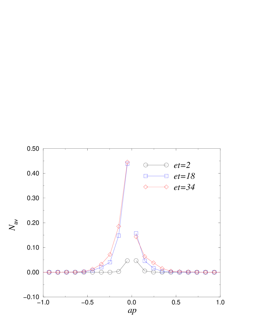
Figure 3: Time dependent particle number $N_{\rm av}$ versus $ap$, the momentum in lattice units, at three different times. The particle numbers are obtained from a time average over an interval of length $et_{\rm av}=4$ and $et$ denotes the center of the interval.

The result for the averaged particle number is shown in fig. 3. The particle numbers of the modes with $|ap|>1$ are consistent with zero, up to numerical precision. These modes are not excited at all. As can be seen from fig. 3, essentially only the physical (i.e. without lattice artefacts) fermions (with $|ap|\raisebox{-1.29167pt}{$\enskip\stackrel{{\scriptstyle<}}{{\scriptstyle\sim}}\enskip$}0.5$) are excited. Furthermore the distributions are much smoother than those obtained with homogeneous mean fields [5, 6]. Note that the distribution functions are not symmetric under $p\to-p$. This will be discussed below.

With respect to the time dependent mass $m_{p}(t)$ in (3.8–3.10), we find no significant deviation from the free dispersion relation $E=|p|$. Finally, we find that ${\cal V}_{0{\rm av}}(p,t)-1/2$ and ${\cal P}_{\rm av}(p,t)$ are consistent with zero for momenta $|ap|>0.5$. For smaller momenta they fluctuate around zero. The amplitude in the case of ${\cal P}_{\rm av}(p,t)$ is smaller than $0.005$.

In order to see whether the fermion subsystem effectively thermalizes locally in time we compare it with the Fermi-Dirac distribution function, depending on a time dependent temperature $T(t)=1/\beta(t)$ and chemical potential $\mu(t)$,

$$f_{p}(t)=\frac{1}{\exp[\beta(t)(E_{p}-\mu(t)q_{5p})]+1}.$$ (4.1)

The chemical potential is coupled to the axial charge density, and we use the notation $q_{5p}=\mbox{sign}(p)=\mbox{sign}(\gamma_{5})$ to denote the chirality. Note that this term breaks the symmetry $p\to-p$. In thermal and chemical equilibrium $N_{p}(t)=\bar{N}_{-p}(t)=N_{{\rm av}p}(t)=f_{p}(t)$.

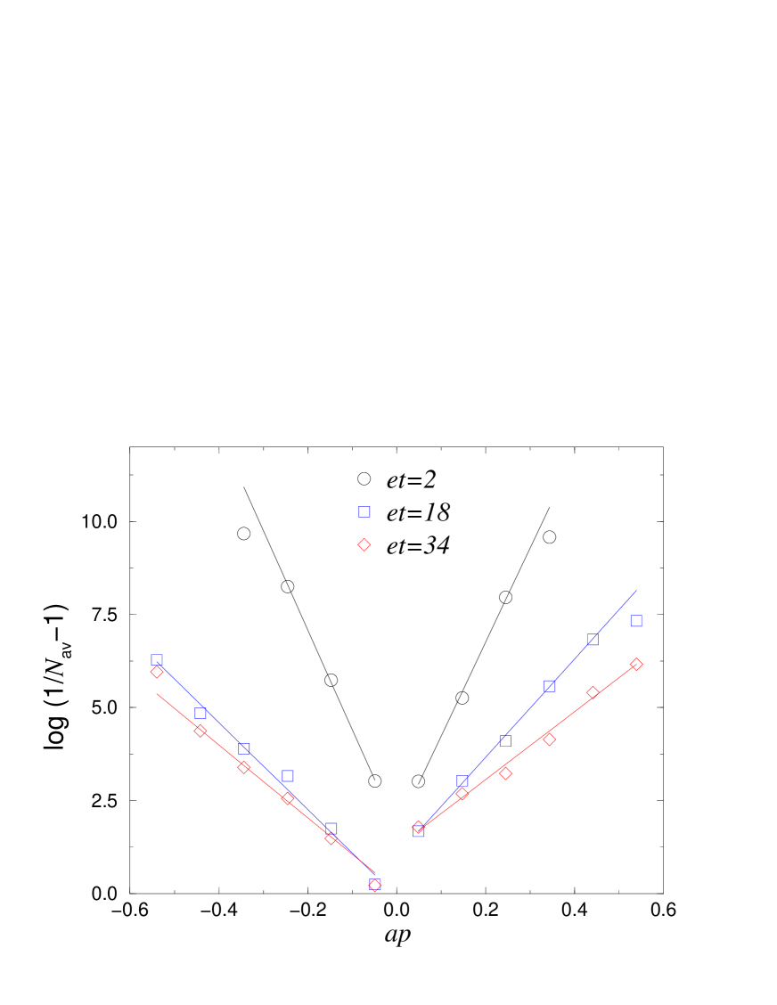
Figure 4: Transformed particle number $\log(N^{-1}_{\rm av}-1)$ for the data of fig. 3. In equilibrium this would give $\beta(t)[|p|\pm\mu(t)]$. The lines are obtained from a straight line fit.

To compare the particle numbers with the Fermi-Dirac distribution, we plot $\log(N^{-1}_{\rm av}-1)$ versus $ap$. In equilibrium this would result in a straight line $\beta(t)[|p|\pm\mu(t)]$. The results are shown in fig. 4. We see that the points seem to lie approximately on straight lines, with small deviations present. The lines through the points are obtained from a straight line fit. Note that the data denoted with $et=2$ represent the averaged particle number in the first interval, $0<et<4$, which contains less than 1.5 oscillations of the Chern-Simons number (see fig. 1). Already here the low momentum modes show approximate thermalization.

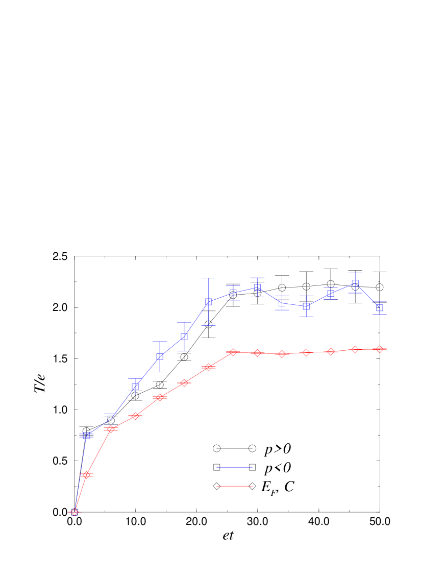
Figure 5: Time dependent effective temperature versus $et$, obtained from least square fits (with errors) from the transformed particle numbers as in fig. 4, for $p>0,p<0$ separately. The line denoted with $E_{F},C$ is obtained from (4.2), i.e. assuming  that the fermions are in thermal and chemical equilibrium.

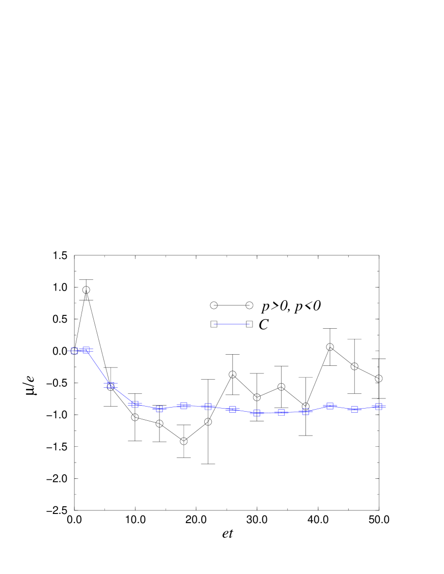
Figure 6: Time dependent effective chemical potential versus $et$, obtained as in the previous figure. Here the result is averaged over the chemical potentials obtained from the $p>0$ and $p<0$ fits. The line denoted with $C$ is again obtained from (4.2).

From least square fits to the data we can find the time dependent temperature and chemical potential, with errors. The effective temperature is obtained separately from $p>0$ and $p<0$ distribution functions and is shown in fig. 5. The effective chemical potential is shown in fig. 6. In this case we present the average of the chemical potential obtained from the $p>0$ and $p<0$ distribution functions, since the fluctuations are rather large. The errors correspond to the least squares fit.

If the fermions are in thermal and chemical equilibrium, with possibly slowly varying time dependent temperature and chemical potential, and interactions are neglected, the relation between $\langle Q_{5}\rangle$, $E_{F}$, $T$ and $\mu$ is as follows. For massless fermions, $E_{p}=|p|$, we find that in that case the axial charge is given by

$$\frac{\langle Q_{5}\rangle}{L}=n_{f}\int_{-\infty}^{\infty}\frac{dp}{2\pi}q_{5p}\left[\frac{1}{e^{\beta(E_{p}-\mu q_{5p})}+1}-\frac{1}{e^{\beta(E_{p}+\mu q_{5p})}+1}\right]\\ =n_{f}\frac{\mu}{\pi}.$$

With the help of the anomaly equation, $\langle Q_{5}\rangle=n_{f}C$, this gives $\mu$ in terms of $C$. Likewise, the renormalized fermion energy at finite temperature and chemical potential can be calculated,

$$\frac{E_{F}}{L}=n_{f}\left(\frac{\pi}{6}T^{2}+\frac{1}{2\pi}\mu^{2}\right),\;\;\;\;\mu=\frac{\pi C}{L}.$$ (4.2)

Given $C$ and $E_{F}$, we can predict $T$ and $\mu$ assuming  the fermions are in equilibrium and neglecting interactions. This predictions are shown in figs. 5 and 6 as well. (Here the error is the standard deviation of the average in an interval $et_{\rm av}=4$, treating the data as uncorrelated.) We see that the equilibrium temperature obtained from (4.2) lies significantly below the effective temperatures obtained from the particle distribution functions. Presumably this reflects the fact that the fermions are of course not really free.

The chemical potential from the fits has large fluctuations and errors. This is possibly due to finite size effects. The time independent equilibrium result (4.2) suggests that the chemical potential will be sensitive to time dependence of the Chern-Simons number (see fig. 1). This dependence should decrease when the volume $L$ gets larger.

5 Conclusion

We presented numerical results for fermion particle production in the presence of inhomogeneous time dependent Bose fields. The quantum field dynamics was approximated by effective mean field equations of motion for the Bose fields coupled to quantized fermion fields, represented by mode functions. The particle number was extracted from the single-time Wigner function, using the free Wigner function as a guideline. For strongly coupled theories, such an approach would presumably not be possible.

A comparison of the particle number with a time dependent Fermi-Dirac distribution, i.e. containing a time dependent temperature and chemical potential, showed that the produced particles are approximately in thermal equilibrium, already after the first few oscillations of the Bose fields. The effective temperature increases when more energy is transferred towards the fermion degrees of freedom. Note that these results are quite different from those obtained with only homogeneous Bose fields, in which case particle distributions are typically non-thermal. Due to the inhomogeneous gauge field, the equations studied here contain classical (screened) Coulomb scattering of the particle-like modes, whereas this is absent in the case of homogeneous mean fields, for which mode coupling is severely reduced.

In this paper our main focus was on fermion particle production. An analysis of the complete system, e.g. of the time dependent energy distribution of the Bose fields, remains to be done.

This study may be relevant for inflationary scenarios. Preheating of the universe is usually analysed by coupling the homogeneous inflaton field to the particle mode functions, leading to resonance band structures and highly non-thermal particle distribution functions (see e.g. references given in the Introduction). The stability of these resonance bands and the time scales of thermalization will be affected when inhomogeneities are taken into account.

Acknowledgments

We thank Bert-Jan Nauta and Henk Stoof for useful discussions. This work is supported by FOM.

A Lattice implementation

We solve the effective equations numerically, using a formulation of the theory on a lattice in space and time. For details concerning especially the fermion fields we refer to [7], here we repeat only the necessary. We use a lattice in space with $N$ sites and lattice spacing $a$, such that $L=Na$. The index $p$ labeling the mode functions then takes a finite number of values

$$p=\frac{2\pi}{L}(n-\frac{1}{2}),\;\;\;\;n\in\{-\frac{1}{2}N+1,\ldots,\frac{1}{2}N\},$$ (A.1)

and the total number of mode functions is given by $2n_{f}N=4N$. On the lattice the dispersion relation is modified and reads for massless Wilson fermions [7]

$$E_{p}=\sqrt{s_{p}^{2}+m_{p}^{2}},\;\;\;\;s_{p}=a^{-1}\sin ap,\;\;\;\;m_{p}=a^{-1}(1-\cos ap),$$ (A.2)

where $m_{p}$ is the ‘Wilson mass’. The maximal fermion momentum on the lattice equals $ap=\pi(1-1/N)\simeq\pi$, in units of the lattice spacing. For such high momenta lattice artefacts are important. The physical modes are those with momenta that are small in lattice units, since then $E_{p}=|p|(1+{\cal O}(a^{2}p^{2}))$. A rough guideline is $|ap|\raisebox{-1.29167pt}{$\enskip\stackrel{{\scriptstyle<}}{{\scriptstyle\sim}}\enskip$}0.5$, for $ap=0.5$ the correction term is approximately $1\%$. The time step is denoted with $a_{0}$. The lattice parameters are $N=64$ and $a_{0}/a=0.005$.

B Numerical calculation of the Wigner function

In this appendix we describe how we calculate the Wigner function numerically on the lattice. We also compare the single-time Wigner function with the gauge fixed equal-time two-point function.

While the definition of the Wigner function is manifestly gauge invariant, it is particularly convenient to calculate it in the (completely gauge fixed) Coulomb gauge. We define this (suppressing the time dependence) by

$$A_{1}^{c}=A_{1}(x)+\partial_{1}\theta_{c}(x),\;\;\;\;\partial_{1}A_{1}^{c}=0,\;\;\;\;-1<C_{c}\leq 1,$$ (B.1)

where the gauge fixed Chern-Simons number is $C_{c}=-LA_{1}^{c}/(2\pi)$. This completely fixes the gauge. In particular the freedom under large gauge transformations is fixed by the last requirement in (B.1). We recall that due the $q=\frac{1}{2}$ charged fermions, $C=1$ is not gauge equivalent to $C=0$, but e.g. to $C=-1$. The fermion fields transform accordingly $\psi(x)\to\psi_{c}(x)=\exp[iq\theta_{c}(x)]\psi(x)$. The parallel transporter in the Wigner function is in this gauge simply $U(y,x;t)=\exp\left[iqA_{1}^{c}(y-x)\right]$.

The Wigner function, averaged over the lattice in space, becomes

$$W(p,t)=\frac{1}{L}\sum_{X}\sum_{z}e^{-i(p+qA_{1}^{c})z}\langle\psi_{c}(X+\frac{1}{2}z,t)\bar{\psi}_{c}(X-\frac{1}{2}z,t)\rangle.$$ (B.2)

Up to the factor $\exp\left[-iqA_{1}^{c}z\right]$, this is identical to what would have been obtained when started from the Coulomb gauge fixed propagator. To evaluate it, we first calculate the Fourier transform of the gauge fixed two-point function

$$S(p,t)=\sum_{z}e^{-ipz}\frac{1}{L}\sum_{X}\langle\psi_{c}(X+\frac{1}{2}z,t)\bar{\psi}_{c}(X-\frac{1}{2}z,t)\rangle,$$ (B.3)

which is the discrete Fourier transform of an antiperiodic function. Hence we know $S(p,t)$ at a discrete set of $p$ values, namely those given by (A.1). Using inter- and extrapolation, the value of $S(p,t)$ at other values of $p$ can be found as well. It follows from comparing (B.2) and (B.3) that the Wigner function is given by $W(p,t)=S(p+qA_{1}^{c},t)$.

The gauge fixed propagator shows discontinuous behaviour when the Chern-Simons number crosses the boundaries set by fixing the freedom under large gauge transformations in (B.1). We expect these discontinuities to become less important when the volume is increased. On the other hand, the presence of the time dependent phase factor in (B.2) leads to a smooth behaviour of the Wigner function when the Chern-Simons number changes during time evolution.

Finally, the explicit expressions for the time dependent particle number $N_{p}$(t), the antiparticle number $\bar{N}_{p}(t)$ and the effective mass $m_{p}(t)$ in terms of the functions ${\cal F}_{\rm av}(p,t)$ and ${\cal V}_{\mu\rm av}(p,t)$ can be obtained as follows. First note from (3.8) and (3.9) that

$${\cal F}_{\rm av}^{2}(p,t)+{\cal V}_{1\rm av}^{2}(p,t)=\frac{1}{4}\left(1-N_{p}-\bar{N}_{-p}\right)^{2},$$

which gives $|1-N_{p}-\bar{N}_{-p}|$. The sign can be found from (3.9), and

$$N_{{\rm av}p}(t)=\frac{1}{2}(N_{p}+\bar{N}_{-p})=\mbox{sign}[p{\cal V}_{1\rm av}(p,t)]\sqrt{{\cal F}_{\rm av}^{2}(p,t)+{\cal V}_{1\rm av}^{2}(p,t)}+\frac{1}{2}.$$

The individual (anti)particle numbers (instead of the sum) can be found by adding or subtracting

$$-{\cal V}_{0\rm av}(p,t)+\frac{1}{2}=\frac{1}{2}(N_{p}-\bar{N}_{-p}).$$

The effective mass, or more generally the dispersion relation, can then be found from

$$\sqrt{m_{p}^{2}(t)+p^{2}}=\frac{p\left(N_{{\rm av}p}(t)-\frac{1}{2}\right)}{{\cal V}_{1\rm av}(p,t)},$$

provided ${\cal V}_{1\rm av}(p,t)\neq 0$ of course. However, ${\cal V}_{1\rm av}(p,t)$ vanishes only when $N_{{\rm av}p}(t)-\frac{1}{2}$ equals zero as well, since the momentum $p$ on the lattice is always different from zero, due to the antiperiodic boundary conditions in space (see (A.1)). Note that since ${\cal F}_{\rm av}(p,t)$ and ${\cal V}_{1\rm av}(p,t)$ are both real, ${\cal F}_{\rm av}(p,t)/{\cal V}_{1\rm av}(p,t)=-m_{p}(t)/p$ is real as well, which implies that $m_{p}(t)$ is real.

References

- [1] F. Cooper, S. Habib, Y. Kluger, E. Mottola, J. P. Paz and P. R. Anderson, Phys. Rev. D50 (1994) 2848.
- [2] Y. Kluger, J. M. Eisenberg, B. Svetitsky, F. Cooper and E. Mottola, Phys. Rev. Lett. 67 (1991) 2427; F. Cooper, S. Habib, Y. Kluger and E. Mottola, Phys. Rev. D55 (1997) 6471.
- [3] D. Boyanovsky, H. J. de Vega, R. Holman and J. F. J. Salgado, Phys. Rev. D54 (1996) 7570; D. Boyanovsky, D. Cormier, H. de Vega, R. Holman, A. Singh and M. Srednicki, Phys. Rev. D56 (1997) 1939.
- [4] D. Boyanovsky, C. Destri, H. J. de Vega, R. Holman and J. Salgado, Phys. Rev. D57 (1998) 7388.
- [5] Y. Kluger, J. M. Eisenberg, B. Svetitsky, F. Cooper and E. Mottola, Phys. Rev. D45 (1992) 4659.
- [6] D. Boyanovsky, M. D’Attanasio, H. J. de Vega, R. Holman and D. S. Lee, Phys. Rev. D52 (1995) 6805; J. Baacke, K. Heitmann and C. Pätzold, Phys. Rev. D58 (1998) 125013.
- [7] G. Aarts and J. Smit, Nucl. Phys. B555 (1999) 355.
- [8] L. M. A. Bettencourt and C. Wetterich, Phys. Lett. B430 (1998) 140.
- [9] D. Y. Grigoriev and V. A. Rubakov, Nucl. Phys. B299 (1988) 67.
- [10] S. Y. Khlebnikov and I. I. Tkachev, Phys. Rev. Lett. 77 (1996) 219.
- [11] For recent reviews, see e.g., V. A. Rubakov and M. E. Shaposhnikov, Usp. Fiz. Nauk 166 (1996) 493; M. Trodden, hep-ph/9803479.
- [12] J. García-Bellido, D. Grigoriev, A. Kusenko and M. Shaposhnikov, hep-ph/9902449.
- [13] P. B. Greene and L. Kofman, Phys. Lett. B448 (1999) 6; G. F. Giudice, M. Peloso, A. Riotto and I. Tkachev, JHEP 08 (1999) 014.
- [14] L. Kofman, A. Linde and A. A. Starobinsky, Phys. Rev. D56 (1997) 3258.
- [15] D. Vasak, M. Gyulassy and H. T. Elze, Ann. Phys. 173 (1987) 462.
- [16] J. P. Blaizot and E. Iancu, Nucl. Phys. B390 (1993) 589; Phys. Rev. Lett. 70 (1993) 3376; Nucl. Phys. B417 (1994) 608.
- [17] P. Zhuang and U. Heinz, Ann. Phys. 245 (1996) 311; S. Ochs and U. Heinz, Ann. Phys. 266 (1998) 351.
- [18] D. Ibaceta and E. Calzetta, hep-ph/9810301.