Short Distance Analysis of $\bar{B}\to D^{(\ast)0}e^{+}e^{-}$ and $\bar{B}\to J/\psi e^{+}e^{-}$

Abstract

Over a large fraction of phase space a combination of an operator product and heavy quark expansions effectively turn the decay $\bar{B}\to D^{(\ast)0}e^{+}e^{-}$ into a “short distance” process, i.e., one in which the weak and electromagnetic interactions occur through single local operators. These processes have an underlying W-exchange quark diagram topology and are therefore Cabibbo allowed but suppressed by combinatoric factors and short distance QCD corrections. Our technique allows a clearer exploration of these effects. For the decay $\bar{B}_{d,s}\to J/\psi(\eta_{c})e^{+}e^{-}$ one must use a non-relativistic (NRQCD) expansion, in addition to an operator product expansion and a heavy quark effective theory expansion. We estimate the decay rates for $\bar{B}_{d,s}\to J/\psi e^{+}e^{-}$, $\bar{B}_{d,s}\to\eta_{c}e^{+}e^{-}$, $\bar{B}_{d,s}\to D^{*0}e^{+}e^{-}$ and $\bar{B}_{d,s}\to D^{0}e^{+}e^{-}$.

PACS numbers: 13.20.He, 12.39.Hg

I Introduction

In a recent paper[1] we considered the collection of decays $B^{+}\to D_{s,d}^{(*)+}e^{+}e^{-}$. The decay rate for these is proportional to $|V_{ub}|^{2}$. We found that over a large kinematic domain one can reliably estimate the rate (in terms of $|V_{ub}|^{2}$). The process is first order weak and first order electromagnetic, and, therefore, the amplitude involves long distance physics. The central observation of [1] is that over a large kinematic domain the interaction is local on the scale of strong dynamics. The amplitude can, therefore, be approximated by the matrix elements of local operators, which can be estimated in a variety of ways and should eventually be determined in numerical simulations of QCD on the lattice. The branching fraction for $B^{+}\to D_{s}^{*+}e^{+}e^{-}$, restricted to invariant mass of the $e^{+}e^{-}$ pair in excess of $1.0$ GeV, was estimated to be $1.9\times 10^{-9}$. This is too small to be measured in $e^{+}e^{-}$ B-factories, but could be observable at high luminosity high energy hadronic colliders.

In this paper we consider the decays $\bar{B}_{s,d}\to J/\psi e^{+}e^{-}$, $\bar{B}_{s,d}\to\eta_{c}e^{+}e^{-}$, $\bar{B}_{s,d}\to D^{*0}e^{+}e^{-}$ and $\bar{B}_{s,d}\to D^{0}e^{+}e^{-}$. These proceed via W-exchange topologies, as shown in Fig. 1. In addition, $\bar{B}_{d,s}\to J/\psi e^{+}e^{-}$ and $\bar{B}_{d,s}\to\eta_{c}e^{+}e^{-}$ have small contributions from penguins, which we neglect. The goal of the paper is to show how the methods introduced in paper[1] can be applied to the processes considered here. The kinematics of $\bar{B}_{d,s}\to D^{(*)0}e^{+}e^{-}$ is similar to that of $B^{+}\to D_{d,s}^{(*)+}e^{+}e^{-}$ so one expects the methods to apply readily. In fact, the only dynamical difference is that in $\bar{B}_{d,s}\to D^{(*)0}e^{+}e^{-}$ the heavy $b$ quark decays to a heavy $c$-quark, whereas in $B^{+}\to D_{s,d}^{(*)+}e^{+}e^{-}$ it is a heavy $b$-anti-quark that decays into a heavy $c$-quark. The case $\bar{B}_{d,s}\to J/\psi(\eta_{c})e^{+}e^{-}$ is clearly different: both quark and anti-quark in the final state are heavy and they are moving together in a bound charmonium state. As we will see the expansion that arises naturally corresponds to NRQCD, the non-relativistic limit of heavy quarks bound by QCD into quarkonia.

The processes under consideration here have advantages compared to $B^{+}\to D_{s,d}^{(*)+}e^{+}e^{-}$. These processes are not suppressed by the small CKM element $|V_{ub}|^{2}$. One might hope that the decay rate is, therefore, substantially higher. However, the enhancement of the rate due to bigger CKM elements is partially cancelled by small Wilson coefficients. Therefore, all these processes have small branching fractions. While none are observable at B-factories, some are observable at future hadronic collider experiments like LHC-B and BTeV.

These processes are first order weak and first order electromagnetic, and, therefore, the amplitude involves long distance physics. We will show that over a large kinematic domain the interaction is approximated by a set of matrix elements of local operators. All these matrix elements should eventually be determined by lattice calculations. For the processes considered in this paper, the number of independent matrix elements is reduced by the use of rotational, heavy quark spin and chiral symmetries.

FIG. 1.: W-exchange quark topology diagram underlying the transition $\bar{B}_{d,s}\to D^{(*)0}e^{+}e^{-}$. Emission of a $e^{+}e^{-}$ pair from any line is understood.

This paper is organized as follows. In Sec. II we review the methods of Ref. [1] that lead to an expansion in local operators. The review is done in terms of the graphs relevant to $\bar{B}\to D^{0}e^{+}e^{-}$, which is one of the processes of interest here. In Sec. III we present a novel analysis that shows that the matrix elements of the operators in the expansion are all related by a combination of heavy-spin, rotational and chiral symmetries. We then proceed to find the short distance QCD corrections to our operator expansion in Sec. IV. In Sec. V we give expressions for the differential decay rates in terms of matrix elements of local operators. These should be considered our main results. To get some numerical estimates of the decay rates we crudely approximate the local matrix elements. The material in Secs. II–V deals with the decays $\bar{B}_{q}\to D^{*0}e^{+}e^{-}$ and $\bar{B}_{q}\to D^{0}e^{+}e^{-}$, and we repeat the steps applied to the processes $B_{q}\to\eta_{c}e^{+}e^{-}$ and $B_{q}\to J/\psi e^{+}e^{-}$ in Sec. VI. Our results are summarized in Sec. VII.

II Operator Expansion

In this section we review the method introduced in [1]. However, we will present the method as applied to the process $\bar{B}_{d}\to D^{(*)0}e^{+}e^{-}$. Therefore we will at once review the method and perform the necessary calculation for one of the cases of interest.

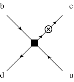
FIG. 2.: Feynman diagram representing a contribution to the Green function. The filled square represents the four quark operator ${\cal O}$ and the cross represents the electromagnetic current $j^{\mu}_{{\rm em}}$, cf. Eq. (4), which here couples to the $c$-quark.

The effective Hamiltonian for the weak transition in $\bar{B}_{d}\to D^{(*)0}e^{+}e^{-}$, is

$${\cal H}^{\prime}_{\rm eff}=\frac{4G_{F}}{\sqrt{2}}\,V^{\phantom{*}}_{ud}V^{*}_{cb}\left(c(\mu/M_{W}){\cal O}+c_{8}(\mu/M_{W}){\cal O}_{8}\right),$$ (1)

where

$${\cal O}=\bar{d}\gamma^{\nu}P_{-}b\;\;\bar{c}\gamma_{\nu}P_{-}u$$ (2)

and

$${\cal O}_{8}=\bar{d}\gamma^{\nu}P_{-}T^{a}b\;\;\bar{c}\gamma_{\nu}P_{-}T^{a}u,$$ (3)

$P_{\pm}\equiv(1\pm\gamma_{5})/2$ and $T^{a}$ are the generators of color gauge symmetry. This is a useful basis of operators for our purposes since the hadronic matrix element of the “octet” operator ${\cal O}_{8}$ is suppressed. The dependence on the renormalization point $\mu$ of the short distance coefficients $c$ and $c_{8}$ cancels the $\mu$-dependence of operators, so matrix elements of the effective Hamiltonian are $\mu$-independent.

The amplitude for $\bar{B}_{d}\to D^{(*)0}e^{+}e^{-}$, to leading order in weak and electromagnetic interactions and to all orders in the strong interactions involves the following non-local matrix element:

$$\langle D^{*+}|\int d^{4}x\;e^{iq\cdot x}\;T(j^{\mu}_{\rm em}(x){\cal O}(0))|B^{+}\rangle.$$ (4)

Here $q$ denotes the momentum of the $e^{+}e^{-}$ pair, $j^{\mu}_{\rm em}$ is the electromagnetic current operator and the operator ${\cal O}$, defined in Eq. (2), is the long distance approximation to the $W$-exchange graph. The full amplitude will of course also involve a similar non-local matrix element but with the “singlet” operator ${\cal O}$ replaced by the octet operator ${\cal O}_{8}$. For now we concentrate on the singlet operator. None of the arguments given in this section depend on the particular choice of the operator.

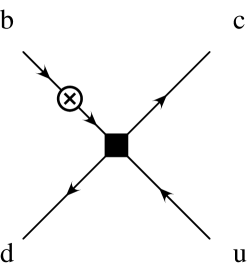
FIG. 3.: Same as Fig. 2 but with the electromagnetic current coupling to the $b$-quark.

We will now argue that for heavy $b$ and $c$ quarks the non-local matrix element in Eq. (4) is well approximated by the matrix element of a sum of local operators. The approximation is valid provided ${\Lambda_{\rm QCD}}\ll m_{c,b}$, i.e., the corrections are order ${\Lambda_{\rm QCD}}/m_{c,b}$. There are also corrections of order ${\Lambda_{\rm QCD}}m_{b,c}/q^{2}$. So our results are limited to the region were $q^{2}$ scales like $m_{c,b}^{2}$. The region were $q^{2}$ does not scale like $m_{c,b}^{2}$ is parametrically small, so the arguments we present are theoretically sound. However, there is the practical issue of determining a minimum $q^{2}$ for realistic calculations were our approximations can still be trusted. We return to this practical matter below, when we attempt to estimate the rate for this decay.

The underlying decay is represented in the quark diagrams of Figs. 2–5. In the heavy quark limit, ${\Lambda_{\rm QCD}}\ll m_{c,b}$, the heavy meson momentum is predominantly the heavy quark’s. This suggests the following kinematics in the quark diagrams: for the momenta of the heavy quarks take $m_{b}v+k_{b}$ and $m_{c}v^{\prime}+k_{c}$, for the momenta of the light quarks take $k_{u}$ and $k_{d}$ and then the photon’s momentum is determined by conservation, $q=m_{b}v-m_{c}v^{\prime}+\sum k_{i}$. We can now exhibit our OPE by considering the quark Green functions in Figs. 2–5. The convergence of the expansion for physical matrix elements rests on the intuitive fact that the residual momenta $k_{i}$ will be of order ${\Lambda_{\rm QCD}}$ (parametrically all we need is that these are independent of the large masses). This intuition is made explicit in Heavy Quark Effective Theory (HQET): there are no heavy masses in the HQET-Lagrangian so the only relevant dynamical scale is ${\Lambda_{\rm QCD}}$. Thus our expansion of a non-local product will be in terms of local operators of the HQET.

FIG. 4.: Same as Fig. 2 but with the electromagnetic current coupling to the $u$-quark.

Calculating the Feynman diagram of Fig. 2 with our choice of kinematics we have

$$-iQ_{c}\gamma^{\mu}\frac{i}{q\hskip-5.0pt/+m_{c}v\hskip-5.0pt/^{\prime}+k\hskip-5.0pt/_{c}-m_{c}}\gamma^{\nu}P_{-}\otimes\gamma_{\nu}P_{-}.$$ (5)

Here $Q_{c}=2/3$ is the charge of the $c$-quark and the tensor product corresponds to the two fermion bilinears. External legs are amputated. Using $q=m_{b}v-m_{c}v^{\prime}+\sum k_{i}$ and expanding in $k_{i}/m_{c,b}$ we obtain, to leading order

$$Q_{c}\gamma^{\mu}\frac{m_{b}v\hskip-5.0pt/+m_{c}}{m_{b}^{2}-m_{c}^{2}}\gamma^{\nu}P_{-}\otimes\gamma_{\nu}P_{-}.$$ (6)

This Green’s function is that of a local operator in the HQET. Denoting by $h_{v}^{(Q)}$ the annihilation operator for the heavy quark with four-velocity $v$, we define

$$\tilde{\cal O}\equiv\bar{d}\Gamma^{\phantom{()}}_{b}h^{(b)}_{v}\;\bar{h}^{(c)}_{v^{\prime}}\Gamma^{\phantom{()}}_{c}u.$$ (7)

Here $\Gamma_{b,c}$ are arbitrary Dirac matrices. With $\Gamma_{c}\otimes\Gamma_{b}$ set equal to the tensor product in (6),

$$\Gamma_{c}\otimes\Gamma_{b}=Q_{c}\gamma^{\mu}\frac{m_{b}v\hskip-5.0pt/+m_{c}}{m_{b}^{2}-m_{c}^{2}}\gamma^{\nu}P_{-}\otimes\gamma_{\nu}P_{-},$$ (8)

the operator expansion is

$$\int d^{4}x\;e^{iq\cdot x}\;T[\bar{c}\gamma^{\mu}c(x)\;{\cal O}(0)]=\tilde{\cal O}+\cdots.$$ (9)

The ellipses indicate terms of higher order in our expansion, and correspond to higher derivative operators suppressed by powers of $m_{c,b}$. There are also perturbative corrections to this expression. These show up as modifications to the operator defined by setting $\Gamma_{c}\otimes\Gamma_{b}$ equal to (6).

FIG. 5.: Same as Fig. 2 but with the electromagnetic current coupling to the $d$-quark.

The diagram of Fig. 3 can be analyzed in complete analogy. It leads to the operator $\tilde{\cal O}$ with the choice

$$\Gamma_{c}\otimes\Gamma_{b}=-Q_{b}\gamma^{\nu}P_{-}\otimes\gamma_{\nu}P_{-}\frac{m_{b}+m_{c}v\hskip-5.0pt/^{\prime}}{m_{b}^{2}-m_{c}^{2}}\gamma^{\mu},$$ (10)

where $Q_{b}=-1/3$ is the $b$ quark charge.

The analysis of Figs. 4 and 5 is similar, but there is an important distinction. With the electromagnetic current coupling to the light quarks, we get intermediate light quark propagators. The denominator in these propagators are parametrically large only if $q^{2}$ is parametrically large, i.e., if $q^{2}\sim m_{c,b}^{2}$. With this caveat, the OPE for Fig. 4 gives

$$\Gamma_{c}\otimes\Gamma_{b}=-Q_{u}\gamma^{\nu}P_{-}\frac{q\hskip-5.0pt/}{q^{2}}\gamma^{\mu}\otimes\gamma_{\nu}P_{-}$$ (11)

and for Fig. 5 the OPE gives

$$\Gamma_{c}\otimes\Gamma_{b}=Q_{d}\gamma^{\nu}P_{-}\otimes\gamma^{\mu}\frac{q\hskip-5.0pt/}{q^{2}}\gamma_{\nu}P_{-}.$$ (12)

III Spin Symmetry

We have shown how to replace the time ordered product in Eq. (4) by a local operator. The replacement is valid provided the invariant mass of the lepton pair is large, i.e., scales as $q^{2}\sim m_{c,b}^{2}$. The operator $\tilde{\cal O}$ that replaces the time ordered product is defined by Eq. (7), with the tensor $\Gamma_{c}\otimes\Gamma_{b}$ defined as the sum of the contributions in Eqs. (8), (10), (11) and (12). We now show how to relate the matrix element of this operator to the operator with $\Gamma_{c}\otimes\Gamma_{b}=\gamma^{\nu}P_{-}\otimes\gamma_{\nu}P_{-}$. This operator is not only simpler, but one can estimate its matrix elements by a variety of means, as we explain below.

Consider the matrix element of $\tilde{\cal O}$ as defined in Eq. (7) for arbitrary tensor product $\Gamma_{c}\otimes\Gamma_{b}$ between heavy meson states. We will use heavy quark spin symmetry to determine the matrix elements of this operator between heavy meson states. Recall that the HQET lagrangian

$${\cal L}_{\rm HQET}={\bar{h}^{(b)}_{v^{\phantom{\prime}}}}iv\cdot D{h^{(b)}_{v^{\phantom{\prime}}}}+\bar{h}^{(c)}_{v^{\prime}}iv^{\prime}\cdot Dh^{(c)}_{v^{\prime}}$$ (13)

is symmetric under the group $SU(2)_{b}\times SU(2)_{c}$ of transformations acting on spin indices of the heavy quark fields:

$\displaystyle{h^{(b)}_{v^{\phantom{\prime}}}}\to S^{\phantom{\dagger}}_{b}{h^{(b)}_{v^{\phantom{\prime}}}}\quad,\quad h^{(c)}_{v^{\prime}}\to S^{\phantom{\dagger}}_{c}h^{(c)}_{v^{\prime}}.$

At $v^{\prime}=v$ the symmetry is enlarged to $U(4)$, which contains an $SU(2)$ subgroup corresponding to a flavor symmetry. For now we will need only the spin symmetries.

In order to make use of these symmetries, it is convenient to represent a spin multiplet consisting of a pseudoscalar $P$ and a vector meson $V_{\mu}$ by a $4\times 4$ matrix

$$H_{v}=\left(\frac{1+v\hskip-5.0pt/}{2}\right)[V_{\mu}\gamma^{\mu}-P\gamma_{5}].$$ (14)

Then $S_{b}\in SU(2)_{b}$ and $S_{c}\in SU(2)_{c}$ act simply on the left,

$$H_{v}^{(b)}\to S_{b}H_{v}^{(b)}\qquad H_{v^{\prime}}^{(c)}\to S_{c}H_{v^{\prime}}^{(c)},$$ (15)

while an arbitrary rotation $R$ represented by the Dirac matrix ${\cal D}(R)$ acts simultaneously on both multiplets according to

$$H^{(Q)}\to{\cal D}(R)^{\dagger}H^{(Q)}{\cal D}(R).$$ (16)

Consider now the matrix element $\langle{H^{(c)}_{v^{\prime}}|\tilde{\cal O}|H^{(b)}_{v}}\rangle$. It must be linear in the tensors $\Gamma_{c}\otimes\Gamma_{b}$, $H^{(b)}_{v}$ and $H^{(c)}_{v^{\prime}}$. Acting with $SU(2)_{b}$ we see that $\Gamma_{b}\to\Gamma_{b}S_{b}^{\dagger}$ and $H_{v}^{(b)}\to S_{b}H_{v}^{(b)}$, so they enter the matrix element as the product $\Gamma_{b}H_{v}^{(b)}$. A similar argument with $SU(2)_{c}$ gives then

$$\langle{H^{(c)}_{v^{\prime}}|\tilde{\cal O}|H^{(b)}_{v}}\rangle\propto\bar{H}^{(c)}_{v^{\prime}}\Gamma_{c}\otimes\Gamma_{b}H^{(b)}_{v}$$ (17)

Finally, invariance under rotations implies that the remaining four indices must be contracted. There are two possible contractions,

$${\rm Tr}(\bar{H}^{(c)}_{v^{\prime}}\Gamma_{c}){\rm Tr}(\Gamma_{b}H^{(b)}_{v})\quad\hbox{and}\quad{\rm Tr}(\bar{H}^{(c)}_{v^{\prime}}\Gamma_{c}\Gamma_{b}H^{(b)}_{v}).$$ (18)

We now show that the second one is excluded by chiral symmetry. The lagrangian for a massless quark in QCD,

$${\cal L}=\bar{\psi}iD\hskip-6.99997pt/\psi,$$ (19)

is invariant under the chiral symmetry

$$\psi\to e^{i\alpha\gamma_{5}}\psi,$$ (20)

where $\alpha$, the parameter of the transformation, is a real number. Under this symmetry the transformation rule for our tensors is

$$\Gamma_{b}H^{(b)}_{v}\to e^{-i\alpha\gamma_{5}}\Gamma_{b}H^{(b)}_{v}e^{i\alpha\gamma_{5}}$$ (21)

and

$$\bar{H}^{(c)}_{v^{\prime}}\Gamma_{c}\to e^{i\alpha\gamma_{5}}\bar{H}^{(c)}_{v^{\prime}}\Gamma_{c}e^{-i\alpha\gamma_{5}}.$$ (22)

It is seen that the first contraction of indices in (18) is invariant, but the second one is not.

We have shown that heavy quark spin symmetry, rotations and light quark chiral symmetry combine to give

$$\langle{H^{(c)}_{v^{\prime}}|\tilde{\cal O}|H^{(b)}_{v}}\rangle=\frac{1}{4}\beta(w){\rm Tr}(\bar{H}^{(c)}_{v^{\prime}}\Gamma_{c}){\rm Tr}(\Gamma_{b}H^{(b)}_{v}).$$ (23)

We have indicated that the invariant matrix element $\beta$ is a function of $w=v\cdot v^{\prime}$. In general, it is a function of $v$ and $v^{\prime}$. However, since it must be Lorenz invariant and since $v^{2}=v^{\prime 2}=1$, it is a function of $w=v\cdot v^{\prime}$ only.

The octet operator in the HQET,

$$\tilde{\cal O}_{8}\equiv\bar{d}\Gamma^{\phantom{()}}_{b}T^{a}h^{(b)}_{v}\;\bar{h}^{(c)}_{v^{\prime}}\Gamma^{\phantom{()}}_{c}T^{a}u,$$ (24)

has the same spin and heavy flavor symmetry properties as its singlet counterpart. Therefore in complete analogy we can introduce a reduced matrix element $\beta_{8}$:

$$\langle{H^{(c)}_{v^{\prime}}|\tilde{\cal O}_{8}|H^{(b)}_{v}}\rangle=\frac{1}{4}\beta_{8}(w){\rm Tr}(\bar{H}^{(c)}_{v^{\prime}}\Gamma_{c}){\rm Tr}(\Gamma_{b}H^{(b)}_{v}).$$ (25)

The authors of Ref. [3] proposed a relation analogous to Eq. (23) for a $\Delta B=2$ transition. It was noted there that spin symmetry allowed more than one invariant and that, however, all invariants lead to the same symmetry relations. One may wonder if our use of chiral symmetry may help relate the different invariants there. We show that this is not the case. For the $\Delta B=2$ case the analogue of Eq. (17) is

$$\langle{H^{(\bar{b})}_{v}|\tilde{\cal O}_{\Delta B=2}|H^{(b)}_{v}}\rangle\propto\Gamma_{\bar{b}}\bar{H}^{(\bar{b})}_{v}\otimes\Gamma_{b}H^{(b)}_{v},$$ (26)

where $\tilde{\cal O}_{\Delta B=2}=\bar{d}\Gamma^{\phantom{()}}_{\bar{b}}h^{(\bar{b})}_{v}\;\bar{d}\Gamma^{\phantom{()}}_{b}h^{(b)}_{v}$ (note that we define $h^{(\bar{b})}_{v}$ to create a $b$-antiquark). Again, invariance under rotations implies that the remaining four indices must be contracted and, again, there are two possible contractions,

$${\rm Tr}(\Gamma_{\bar{b}}\bar{H}^{(\bar{b})}_{v}){\rm Tr}(\Gamma_{b}H^{(b)}_{v})\quad\hbox{and}\quad{\rm Tr}(\Gamma_{\bar{b}}\bar{H}^{(\bar{b})}_{v}\Gamma_{b}H^{(b)}_{v}).$$ (27)

Chiral symmetry for the antiquark’s meson tensor is just as for the quark’s in Eq. (21),

$$\Gamma_{\bar{b}}\bar{H}^{(\bar{b})}_{v}\to e^{-i\alpha\gamma_{5}}\Gamma_{\bar{b}}\bar{H}^{(\bar{b})}_{v}e^{i\alpha\gamma_{5}}.$$ (28)

Therefore both contractions in (27) are allowed by chiral symmetry. However, it is easy to see that for a class of operators of interest the two contractions are equivalent. If

$\displaystyle\Gamma_{\bar{b}}\otimes\Gamma_{b}=\gamma^{\mu}P_{-}\hat{\Gamma}\otimes\gamma_{\mu}P_{-}$

or

$\displaystyle\Gamma_{\bar{b}}\otimes\Gamma_{b}=\gamma^{\mu}P_{-}\otimes\gamma_{\mu}P_{-}\hat{\Gamma},$

for any arbitrary Dirac matrix $\hat{\Gamma}$ the two contractions are related by Fierz rearrangement. This class of operators includes the $B-\bar{B}$ mixing case studied in Ref. [3].

IV QCD Corrections

Consider the operator expansion in Eq. (9). We have seen that at leading order the operator on the right hand side is given by Eqs. (7)–(8). We now consider the leading-log corrections to this relation. In the large mass limit these are formally the largest, leading corrections to the operator expansion. A renormalization scale $\mu$ must be stipulated for the evaluation of matrix elements of the composite operators on both sides of Eq. (9). It is often convenient to evaluate the matrix elements at a low renormalization point $\mu=\mu_{\rm low}$. This choice makes the matrix elements in the HQET completely independent of the large masses of the heavy quarks. If $\mu_{\rm low}\ll m_{c,b}$ there are large corrections to Eq. (9) in the form of powers of $\alpha_{s}\ln(m_{c,b}/\mu_{\rm low})$. These powers of large logarithms can be summed using renormalization group techniques. The corrections to these “leading-logs” are of order $1/\ln(m_{c,b}/\mu_{\rm low})$ or $\alpha_{s}$. It is important therefore to keep $\mu_{\rm low}$ small, but large enough that perturbation theory remains valid. When we estimate decay rates below, we use $\mu_{\rm low}=1.0$ GeV.

To study the dependence on the renormalization point $\mu$ we take a logarithmic derivative on both sides of Eq. (9). Consider first the left side. Acting with $\mu(d/d\mu)$ on the charm number current $\bar{c}\gamma^{\mu}c$ gives zero, because the current is conserved. The action of $\mu(d/d\mu)$ on the composite four-quark operator is a linear combination of itself and the octet operator. It is therefore convenient to consider instead the linear combination that appears in the effective Hamiltonian (1):

$$\int d^{4}x\;e^{iq\cdot x}\;T[\bar{c}\gamma^{\mu}c(x) (c{\cal O}(0)+c_{8}{\cal O}_{8}(0))]=$$ (30)

$$\tilde{c}\tilde{\cal O}+\tilde{c}_{8}\tilde{\cal O}_{8}+\cdots.$$

The coefficients $c$ and $c_{8}$ are such that the left hand side is $\mu$-independent. This is necessary for the physical amplitude to be independent of the arbitrary choice of renormalization point $\mu$. Therefore our task is to determine the proper $\mu$-dependence for $\tilde{c}$ and $\tilde{c}_{8}$ so that the right hand side is also independent of $\mu$. Therefore, if the operators satisfy

$$\mu\frac{d}{d\mu}\left(\begin{array}[]{c}\tilde{\cal O}\\ \tilde{\cal O}_{8}\\ \end{array}\right)=\gamma\left(\begin{array}[]{c}\tilde{\cal O}\\ \tilde{\cal O}_{8}\\ \end{array}\right),$$ (31)

where $\gamma$ is a $2\times 2$ matrix of anomalous dimensions, then the coefficients must satisfy

$$\mu\frac{d}{d\mu}\left(\begin{array}[]{c}\tilde{c}\\ \tilde{c}_{8}\\ \end{array}\right)=-\gamma^{T}\left(\begin{array}[]{c}\tilde{c}\\ \tilde{c}_{8}\\ \end{array}\right).$$ (32)

Here “$T$” denotes transpose of a matrix.

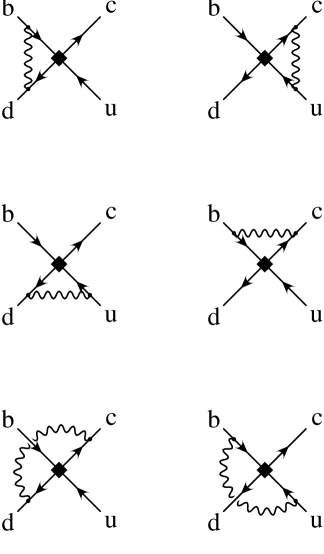
FIG. 6.: One loop Feynman diagrams for the calculation of the anomalous dimension matrix. The solid diamond represents the local operators ${\cal O}$ or ${\cal O}_{8}$.

The calculation of the anomalous dimension matrix is straightforward. In dimensional regularization with $D=4-\epsilon$ dimensions, one needs[4] the residues of the $\epsilon$-poles of graphs with one insertion of the operators $\tilde{\cal O}$ and $\tilde{\cal O}_{8}$. The leading-log corrections arise from the leading, $O(\alpha_{s})$ terms in $\gamma$. These arise from the one-loop graphs in Fig. 6

In principle the different tensor structures $\Gamma_{c}\otimes\Gamma_{b}$ defining $\tilde{\cal O}$ and $\tilde{\cal O}_{8}$ can have different anomalous dimensions and even mix among themselves. However spin symmetry ensures that the anomalous dimension matrix is independent of the tensor structure $\Gamma_{c}\otimes\Gamma_{b}$.

We find

$$\gamma=\frac{\alpha_{s}}{4\pi}\left(\begin{array}[]{cc}8&-4wr(w)-2\\ -\frac{8}{9}wr(w)-\frac{4}{9}&\frac{17}{3}-\frac{14}{3}wr(w))\\ \end{array}\right),$$ (33)

where

$$r(w)\equiv\frac{1}{\sqrt{w^{2}-1}}\ln(w+\sqrt{w^{2}-1}).$$ (34)

The solution to the renormalization group equation (32) is straightforward. In terms of the ratio of running coupling constants

$$z\equiv\left(\frac{\alpha_{s}(\mu)}{\alpha_{s}({{\mu_{0}^{\phantom{\dagger}}}})}\right)$$ (35)

and the functions

$$\psi = \frac{1}{12}\;\frac{41-14wr(w)}{b_{0}},$$ (36)

$$\xi = -\frac{3}{4}\;\frac{1+2wr(w)}{b_{0}},$$ (37)

where the coefficient of the one loop term of the $\beta$-function for QCD is $b_{0}=11-\frac{2}{3}n_{f}$, and $n_{f}$ is the number of light flavors ($n_{f}=3$ in our case), we obtain

$$\left(\begin{array}[]{c}\tilde{c}(\mu)\\ \tilde{c}_{8}(\mu)\\ \end{array}\right)=U\left(\begin{array}[]{c}\tilde{c}({{\mu_{0}^{\phantom{\dagger}}}})\\ \tilde{c}_{8}({{\mu_{0}^{\phantom{\dagger}}}})\\ \end{array}\right)$$ (38)

where

$$U=z^{\psi}\left(\begin{array}[]{cc}\frac{1}{9}z^{\xi}+\frac{8}{9}z^{-\xi}&\frac{4}{27}(z^{\xi}-z^{-\xi})\\ \frac{2}{3}(z^{\xi}-z^{-\xi})&\frac{8}{9}z^{\xi}+\frac{1}{9}z^{-\xi}\end{array}\right).$$ (39)

The question that remains is how to determine the coefficients $\tilde{c}$ and $\tilde{c}_{8}$ at some scale ${{\mu_{0}^{\phantom{\dagger}}}}$. But we have already determined these coefficients in Sec. II. Recall that the operator $\tilde{\cal O}$ that replaces the time ordered product is defined by Eq. (7), with the tensor $\Gamma_{c}\otimes\Gamma_{b}$ defined as the sum of the contributions in Eqs. (8), (10), (11) and (12) with unit coefficient. The question can be rephrased as what is the scale ${{\mu_{0}^{\phantom{\dagger}}}}$ for which the calculation in Sec. II is valid. What we would like to do is to determine for what choice of ${{\mu_{0}^{\phantom{\dagger}}}}$ the loop corrections to relations like Eq. (9) will be free from large logs. The only relevant scales in the problem are the large masses $m_{c,b}$, the invariant mass of the $e^{+}e^{-}$ pair, $q^{2}$, which itself scales like $m_{c,b}^{2}$, the small masses and residual momenta and the renormalization point ${{\mu_{0}^{\phantom{\dagger}}}}$. The corrections to the relations of Sec. II are guaranteed to be free from logs of the small masses or residual momenta. But there will be logs of ratios of large masses to the renormalization point, $\ln(m_{c,b}/{{\mu_{0}^{\phantom{\dagger}}}})$. To avoid these one may choose ${{\mu_{0}^{\phantom{\dagger}}}}\sim m_{c,b}$. For our computations below we will use ${{\mu_{0}^{\phantom{\dagger}}}}\approx 4.0$ GeV. If the scales $m_{c}$ and $m_{b}$ are both large but very disparate one could review the above analysis by introducing a new renormalization group equation to re-sum the logs of $m_{c}/m_{b}$. The results of this section would still re-sum the logs of $\mu/m_{c}$.

We thus have that $\tilde{c}(\mu)$ and $\tilde{c}_{8}(\mu)$ are given by Eqs. (38) and (39), with

$$\tilde{c}({\mu_{0}^{\phantom{\dagger}}}) = c({{\mu_{0}^{\phantom{\dagger}}}})=\frac{2}{3}(x^{-1}-\frac{1}{2}x^{2})$$ (40)

$$\tilde{c}_{8}({{\mu_{0}^{\phantom{\dagger}}}}) = c_{8}({{\mu_{0}^{\phantom{\dagger}}}})=x^{-1}+x^{2}$$ (41)

where

$$x\equiv\left(\frac{\alpha({{\mu_{0}^{\phantom{\dagger}}}})}{\alpha(M_{W})}\right)^{6/23}.$$ (42)

For illustration we have given the leading log expression for the coefficients $c({\mu_{0}^{\phantom{\dagger}}})$ and $c_{8}({{\mu_{0}^{\phantom{\dagger}}}})$, but in rate computations below we use the next to leading log results from [2]. We do not have at present a full next to leading log result: still missing is a computation of the one loop corrections to the coefficients $\tilde{c}$ and $\tilde{c}_{8}$ at $\mu={\mu_{0}^{\phantom{\dagger}}}$ and of the anomalous dimensions matrix $\gamma$ of Eq. (31) at two loops. It is interesting to note that the coefficients $c(\mu_{0})$ are significantly enhanced at next to leading log order. For the case $\mu_{0}=4.0$ GeV one has in next to leading order[2] $c=0.16$, rather than the leading log result $c=0.07$. We emphasize that this enhancement can be systematically accounted for. The large enhancement is not a signal of perturbation theory breaking down but rather due to the accidental cancellation in the leading order.

V Rates: $\bar{B}^{0}\to D^{(*)0}e^{+}e^{-}$

We are ready to compute decay rates. Defining

$$h^{(*)\mu}=\langle D^{(*)0}|\int d^{4}x\;e^{iq\cdot x}\;T(j^{\mu}_{\rm em}(x){\cal H}^{\prime}_{\rm eff}(0))|B^{0}\rangle,$$ (43)

the decay rate for $B^{0}\to D^{(*)0}e^{+}e^{-}$ is given in terms of $q^{2}$ and $t\equiv(p_{D}+p_{e^{+}})^{2}=(p_{B}-p_{e^{-}})^{2}$ by

$$\frac{d\Gamma}{dq^{2}dt}=\frac{1}{2^{8}\pi^{3}M_{B}^{3}}\left|\frac{e^{2}}{q^{2}}\ell_{\mu}h^{(*)\mu}\right|^{2}$$ (44)

where $\ell^{\mu}=\bar{u}(p_{e^{-}})\gamma^{\mu}v(p_{e^{+}})$ is the leptons’ electromagnetic current. A sum over final state lepton helicities, and polarizations in the $D^{*}$ case, is implicit.

To compute $h^{(*)\mu}$ we need to pull together the results of the previous sections. First the time ordered product is expanded in terms of local operators as in Eqs. (8)–(12). This involves replacing the coefficient functions $c({{\mu_{0}^{\phantom{\dagger}}}})$ and $c_{8}({{\mu_{0}^{\phantom{\dagger}}}})$ by $\tilde{c}({{\mu_{0}^{\phantom{\dagger}}}})$ and $\tilde{c}_{8}({{\mu_{0}^{\phantom{\dagger}}}})$ as seen in Eq. (30). Then the matrix elements of the leading local operators $\tilde{\cal O}$ and $\tilde{\cal O}_{8}$ between particular states can all be expressed in terms of the reduced matrix elements $\beta$ and $\beta_{8}$ defined in (23) and (25). Finally, to make all dependence on the heavy quark masses explicit, we run down the coefficients $\tilde{c}$ and $\tilde{c}_{8}$ from the scale $\mu={{\mu_{0}^{\phantom{\dagger}}}}$ of order of $m_{b,c}$ (which we take to be $\sqrt{m_{c}m_{b}}$) to a scale $\mu=\mu_{\rm low}$ of order of a few times ${\Lambda_{\rm QCD}}$.

Our computation gives

$$h^{\mu}=\frac{\kappa}{3} \Big{[}\frac{-(2wm_{b}+m_{c})v^{\mu}-(m_{b}-4wm_{c})v^{\prime\mu}}{(m_{b}v-m_{c}v^{\prime})^{2}}$$ (46)

$$\hskip 85.35826pt+\frac{3(m_{b}v^{\prime\mu}+m_{c}v^{\mu})}{m_{b}^{2}-m_{c}^{2}}\Big{]}$$

and

$$h^{*\mu} = \frac{\kappa}{3}\Big{[}\frac{m_{b}(\epsilon^{\mu}+2v\cdot\epsilon v^{\mu})-m_{c}(3v\cdot\epsilon v^{\prime\mu}+w\epsilon^{\mu})}{(m_{b}v-m_{c}v^{\prime})^{2}}$$ (48)

$$\hskip 56.9055pt+\frac{3im_{c}\epsilon^{\mu\alpha\beta\gamma}\epsilon_{\alpha}v^{\prime}_{\beta}v_{\gamma}}{(m_{b}v-m_{c}v^{\prime})^{2}}$$

$$- \frac{3m_{b}\epsilon^{\mu}+3m_{c}(v\cdot\epsilon v^{\prime\mu}-w\epsilon^{\mu})-im_{c}\epsilon^{\mu\alpha\beta\gamma}\epsilon_{\alpha}v^{\prime}_{\beta}v_{\gamma}}{m_{b}^{2}-m_{c}^{2}}\Big{]}.$$ (49)

Here $\kappa=G_{F}/\sqrt{2}\,V^{\phantom{*}}_{cb}V_{ud}^{*}[\tilde{c}\beta+\tilde{c}_{8}\beta_{8}]$. These expressions are our central results, demonstrating that the decay rates for $B^{0}\to D^{(*)0}e^{+}e^{-}$ can be expressed in terms of the matrix elements $\beta$ and $\beta_{8}$. Below we make an educated guess of these matrix elements, but for reliable results they should be determined from first principles, say, by Monte Carlo simulations of lattice QCD.

In the computation of the rate the amplitude depends on heavy quark masses $m_{c}$ and $m_{b}$, while the phase space involves physical meson masses $M_{B}$ and $M_{D}$ or $M_{D^{*}}$. Although it is straightforward to retain the dependence on all four masses in our expressions for the decay rates, we have chosen to express the results in terms of physical meson masses, with the substitutions $m_{b}=M_{B}$ and $m_{c}=M_{D}$ or $m_{c}=M_{D^{*}}$. We are not justified in distinguishing between quark and meson masses since the distinction enters at higher order in the $1/m_{c,b}$ expansion.

It is now a trivial exercise to compute the differential decay rate. Integrating the rate in Eq. (44) over the variable $t$ we obtain

$$\frac{d\Gamma}{dq^{2}}=\frac{\alpha^{2}G_{F}^{2}}{288\pi M_{B}^{3}}|V_{cb}V_{ud}|^{2}(\tilde{c}\beta+\tilde{c}_{8}\beta_{8})^{2}{\cal F}({\hat{q}}).$$ (50)

Here ${\cal F}({\hat{q}})$ is a dimensionless function of ${\hat{q}}\equiv\sqrt{q^{2}/m_{b}^{2}}$ and ${\hat{m}}\equiv M_{D^{(*)}}/M_{B}$. For $B^{0}\to D^{*0}e^{+}e^{-}$ it is given by

$${\cal F} = \frac{4}{3}\frac{\sqrt{{{1-2{\hat{q}}^{2}-2{\hat{m}}^{2}+{\hat{q}}^{4}-2{\hat{m}}^{2}{\hat{q}}^{2}+{\hat{m}}^{4}}}}}{{\hat{q}}^{6}\hat{m}(1-\hat{m}^{2})^{2}}$$ (54)

$$(5{{\hat{m}}}^{2}+19{{\hat{m}}}^{4}{\hat{q}}^{2}+30{{\hat{m}}}^{6}-20{{\hat{m}}}^{4}-14{\hat{q}}^{2}{{\hat{m}}}^{2}$$

$$-20{{\hat{m}}}^{8}+12{\hat{q}}^{6}{{\hat{m}}}^{2}+{\hat{q}}^{2}+{\hat{q}}^{6}-2{\hat{q}}^{4}+2{{\hat{m}}}^{6}{\hat{q}}^{4}$$

$$-6{{\hat{m}}}^{8}{\hat{q}}^{2}+5{{\hat{m}}}^{10}-6{\hat{q}}^{6}{{\hat{m}}}^{4}+5{{\hat{m}}}^{2}{\hat{q}}^{8}),$$

while for $B^{0}\to D^{0}e^{+}e^{-}$

$${\cal F}=\frac{4(2{\hat{m}}^{2}+1)^{2}(1-2{\hat{q}}^{2}-2{\hat{m}}^{2}+{\hat{q}}^{4}-2{\hat{m}}^{2}{\hat{q}}^{2}+{\hat{m}}^{4})^{\frac{3}{2}}}{3{\hat{q}}^{4}\hat{m}(1-\hat{m}^{2})^{2}}.$$ (56)

In these we have neglected the electron mass.

In order to obtain a numerical estimate of the branching fraction we need to calculate the hadronic matrix elements $\beta$ and $\beta_{8}$. While these could be studied in Monte Carlo simulations of QCD on the lattice, at the moment we have no reliable information on their magnitude. These matrix elements are similar to the matrix element of the $\Delta B=2$ operator for $B-\bar{B}$ mixing. Lattice QCD[5] indicates that the vacuum saturation approximation works very well for $B-\bar{B}$ mixing. Therefore we take vacuum saturation as an educated guess for $\beta$ and $\beta_{8}$. Taking $\Gamma_{c}\otimes\Gamma_{b}=\gamma^{\mu}\gamma_{5}\otimes\gamma^{\nu}\gamma_{5}$ the right hand side of Eq. (23) is $v^{\nu}v^{\prime\mu}\beta$. On the left hand side vacuum saturation gives $(z^{-a_{I}}f_{B}p_{B}^{\nu}/\sqrt{M_{B}})(z^{-a_{I}}f_{D}p_{D}^{\mu}/\sqrt{M_{D}})$. Here $z$ is defined in Eq. (35) and $a_{I}=2/b_{0}$[7] is the well known anomalous scaling power for the heavy-light current in HQET. Thus we obtain

$$\beta(w) = z^{-2a_{I}}f_{B}f_{D}\sqrt{M_{B}M_{D}}$$ (57)

$$\beta_{8}(w) = 0$$ (58)

The second equation is true not just in vacuum saturation but also in the approximation that we can insert a complete set of states between the currents defining $\tilde{\cal O}_{8}$. This is not an exact statement because the composite operator $\tilde{\cal O}_{8}$ does not equal the product of two currents. But the distinction arises from their different short distance behavior. So we expect the deviation of $\beta_{8}$ from zero to be of order of the QCD coupling at short distances $\alpha(\mu_{0})$ times the unsuppressed $\beta$.

Using these matrix elements we integrate the differential rate in Eq. (50) over the range $1.0~{}\hbox{GeV}\leq q^{2}\leq q^{2}_{\rm max}$ to obtain a partial decay rate. We have chosen $q^{2}_{\rm min}=1.0$ GeV as a lower limit since our OPE requires that $q^{2}$ scale like $m_{c,b}^{2}$. The corrections to the leading terms in Eqs. (11) and (12) are of the form of an expansion in $m_{c,b}k/q^{2}$, where $k$ is any of the residual momenta and in our matrix elements is of order ${\Lambda_{\rm QCD}}$. Parametrically, if $q^{2}\sim m_{c,b}^{2}$, then $m_{c,b}k/q^{2}\sim{\Lambda_{\rm QCD}}/m_{c,b}\ll 1$. In addition, the region over which $q^{2}\lesssim{\Lambda_{\rm QCD}}m_{c,b}$ where the expansion breaks down, is parametrically small. However, physical heavy masses are not very large, and the scale $m_{b}{\Lambda_{\rm QCD}}$ is just slightly smaller than $m_{c}^{2}$. In order to have some non-trivial phase space we have taken $q^{2}\gtrsim m_{b}{\Lambda_{\rm QCD}}\sim 1.0$ GeV. The price we pay is that for the lower values of $q^{2}$ our expansion converges slowly, $m_{c,b}k/q^{2}\lesssim 1$.

We find

$${\rm Br}(B^{0}\to D^{*0}e^{+}e^{-})|_{q^{2}>1~{}{\rm GeV}} = 1.4\times 10^{-8}$$ (59)

$${\rm Br}(B^{0}\to D^{0}e^{+}e^{-})|_{q^{2}>1~{}{\rm GeV}} = 2.6\times 10^{-9}$$ (60)

where we have used $|V_{cb}V_{ud}|=0.04$, $f_{D}=f_{B}\sqrt{M_{B}/M_{D}}$ and $f_{B}=170$ MeV. It is important to observe that the portion of phase space $q^{2}\geq 1.0~{}{\rm GeV}$ is expected to give a small fraction of the total rate since the pole at $q^{2}=0$ dramatically amplifies the rate for small $q^{2}$. The rates for $B_{s}^{0}\to D^{*0}e^{+}e^{-}$ and $B_{s}^{0}\to D^{0}e^{+}e^{-}$ can be obtained to good approximation by replacing $|V_{cb}V_{ud}|$ by $|V_{cb}V_{us}|$, reducing the rates by $(0.22)^{2}\approx 0.05$.

The next generation of B-physics experiments at high energy and luminosity hadron colliders, like LHC-B and BTeV, will produce well in excess of $10^{11}$ $B$-mesons per year. Our calculation includes only large invariant mass lepton pairs so detection and triggering on the lepton pair should be straightforward. Dedicated studies must be done to determine feasibility of detection and measurement of spectra of these decays.

VI Decays to Quarkonium

A Operator Expansion and NRQCD

The decays $B_{s}\to\eta_{c}e^{+}e^{-}$ and $B_{s}\to J/\psi e^{+}e^{-}$ (and obvious extensions to excited charmonium) can be studied in a similar way. The notable difference in the operator expansion here is that the residual momenta $k$ of the heavy quarks in the quarkonium bound state do scale with the large heavy mass $k\sim\alpha_{s}m_{c}$, as opposed to the residual momenta of the quarks in the heavy $B$ or $D$ mesons, $k\sim{\Lambda_{\rm QCD}}$. The residual momentum for the case of quarkonia is small for a different reason: ${\bf k}=m_{c}{\bf u}$ and $k^{0}=\frac{1}{2}m_{c}u^{2}$ are small because the velocity ${\bf u}$ of the bound quarks is small[8] for heavy quarks, $u\sim\alpha_{s}(m_{c})$. The parameter of the expansion is therefore $m_{c,b}k/m_{c,b}^{2}\sim\alpha_{s}(m_{c})$.

FIG. 7.: Feynman diagram representing a contribution to the Green function. The filled square represents the four quark operator ${\cal O}$ and the cross represents the electromagnetic current $j^{\mu}_{{\rm em}}$, cf. Eq. (67), which here couples to the $c$-quark.

Our best hope in making the nature of the expansion explicit is to use NRQCD[8], the effective theory of non-relativistic quarks in QCD. As opposed to HQET, where all the heavy mass dependence has disappeared, the lagrangian of NRQCD still depends on the heavy mass:

$${\cal L}_{\rm NRQCD}=\Psi^{\dagger}(iD_{t}-\frac{{\bf D}^{2}}{2m_{c}})\Psi$$ (61)

Here $\Psi$ denotes a two component spinor field for the $c$-quark. A separate spinor field must be included to describe the antiquark. We have written the lagrangian in the rest-frame of charmonium, but it is straightforward to boost into a moving frame. One relies on the dynamics to generate the small parameter of the expansion. For example, the two terms in ${\cal L}_{\rm NRQCD}$ are of comparable magnitude if, as expected, $D_{t}\sim k^{0}\sim m_{c}\alpha_{s}^{2}$ and $|{\bf D}|\sim|{\bf k}|\sim m_{c}\alpha_{s}$.

The operator expansion is in terms of operators with an HQET quark, a light quark and a pair of NRQCD quark-antiquark. So instead of Eq. (7) we have

$$\tilde{\cal O}\equiv\bar{d}\Gamma^{\phantom{()}}_{b}h^{(b)}_{v}\;\Psi_{c}^{\dagger}\Gamma^{\phantom{()}}_{c}\Psi_{\bar{c}},$$ (62)

where $\Psi_{c}^{\dagger}$ and $\Psi_{\bar{c}}$ create a charm quark and a charm antiquark, respectively. We elect to use four component spinors throughout; the reduction to two components results from algebraic constraints that must be imposed, just as in HQET:

$\displaystyle\Psi=\left(\frac{1+v\hskip-5.0pt/^{\prime}}{2}\right)\Psi$

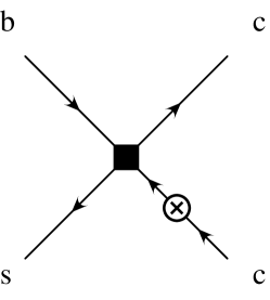
FIG. 8.: Same as Fig. 7 but with the electromagnetic current coupling to the $c$-antiquark.

FIG. 9.: Same as Fig. 7 but with the electromagnetic current coupling to the $b$-quark.

The calculation proceeds much as before. The effective Hamiltonian for the weak transition is

$${\cal H}^{\prime}_{\rm eff}=\frac{4G_{F}}{\sqrt{2}}\,V^{\phantom{*}}_{cs}V^{*}_{cb}\left(c(\mu/M_{W}){\cal O}+c_{8}(\mu/M_{W}){\cal O}_{8}\right),$$ (63)

where

$${\cal O}=\bar{s}\gamma^{\nu}P_{-}b\;\;\bar{c}\gamma_{\nu}P_{-}c$$ (64)

and

$${\cal O}_{8}=\bar{s}\gamma^{\nu}P_{-}T^{a}b\;\;\bar{c}\gamma_{\nu}P_{-}T^{a}c.$$ (65)

The operator expansion of the hadronic matrix element takes the form

$$\int d^{4}x\;e^{iq\cdot x}\;T[j_{\rm em}^{\mu}(x) (c{\cal O}(0)+c_{8}{\cal O}_{8}(0))]=$$ (67)

$$\tilde{c}\tilde{\cal O}+\tilde{c}_{8}\tilde{\cal O}_{8}+\cdots,$$

where $\tilde{\cal O}$ is defined in (62) and the octet operator $\tilde{\cal O}_{8}$ is defined analogously,

$$\tilde{\cal O}_{8}\equiv\bar{d}\Gamma^{\phantom{()}}_{b}T^{a}h^{(b)}_{v}\;\Psi_{c}^{\dagger}\Gamma^{\phantom{()}}_{c}T^{a}\Psi_{\bar{c}}.$$ (68)

The first task is to determine the tensor $\Gamma_{b}\otimes\Gamma_{c}$. To this order we consider Green functions of the time ordered product in Eq. (67) with four external quarks. The in-going momenta of the $b$- and $s$-quarks are $m_{b}v+k_{b}$ and $k_{s}$, respectively. The outgoing momenta of the charm pair are $m_{c}v^{\prime}+k_{c}$ and $m_{c}v^{\prime}+k_{\bar{c}}$. As explained above, we expect $k_{b}\sim k_{s}\sim{\Lambda_{\rm QCD}}$ while $k_{c}\sim k_{\bar{c}}\sim m_{c}\alpha_{s}(m_{c})$. The leading term in the momentum of the electromagnetic current is $q=m_{b}v-2m_{c}v^{\prime}$. For the purpose of determining the expansion coefficients at tree level we may set $c=1$ and $c_{8}=0$ and, choosing a renormalization point ${\mu_{0}^{\phantom{\dagger}}}$ of the order of the large masses $m_{c,b}$, we can set $\tilde{c}=1$ and $\tilde{c}_{8}=0$. There are four graphs contributing to the tensor $\Gamma_{c}\otimes\Gamma_{b}$. Fig. 7 gives

$$\Gamma_{c}\otimes\Gamma_{b}=Q_{c}\gamma^{\mu}\frac{m_{b}v\hskip-5.0pt/-m_{c}(v\hskip-5.0pt/^{\prime}-1)}{m_{b}^{2}-2m_{b}m_{c}w}\gamma^{\nu}P_{-}\otimes\gamma_{\nu}P_{-},$$ (69)

and Fig. 8 gives

$$\Gamma_{c}\otimes\Gamma_{b}=Q_{c}\gamma^{\nu}P_{-}\frac{-m_{b}v\hskip-5.0pt/+m_{c}(v\hskip-5.0pt/^{\prime}+1)}{m_{b}^{2}-2m_{b}m_{c}w}\gamma^{\mu}\otimes\gamma_{\nu}P_{-}.$$ (70)

Note that the denominator, which dictates the convergence of the expansion, scales with $m_{c,b}^{2}$. It vanishes at $w_{0}=m_{b}/2m_{c}$. However, this is never in the physical region: $w_{\rm max}=(m_{b}^{2}+4m_{c}^{2})/4m_{b}m_{c}=w_{0}-(m_{b}/4m_{c}-m_{c}/m_{b})$, but $m_{b}>2m_{c}$ for the decay to be allowed.

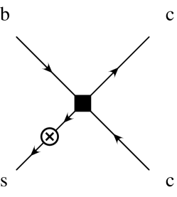
FIG. 10.: Same as Fig. 7 but with the electromagnetic current coupling to the $s$-quark.

The diagrams in Figs. 9 and 10 are just as in Figs. 3 and 5, with the replacement $q=m_{b}v-m_{c}v^{\prime}\to q=m_{b}v-2m_{c}v^{\prime}$. For the first we have

$$\Gamma_{c}\otimes\Gamma_{b}=-Q_{b}\gamma^{\nu}P_{-}\otimes\gamma_{\nu}P_{-}\frac{m_{b}+2m_{c}v\hskip-5.0pt/^{\prime}}{m_{b}^{2}-4m_{c}^{2}}\gamma^{\mu},$$ (71)

and for the second

$$\Gamma_{c}\otimes\Gamma_{b}=Q_{d}\gamma^{\nu}P_{-}\otimes\gamma^{\mu}\frac{q\hskip-5.0pt/}{q^{2}}\gamma_{\nu}P_{-}.$$ (72)

Again we see that the expansion remains valid as long as $q^{2}$ scales with the heavy masses (squared), and this limitation arises solely from the coupling of the photon to the light quark.

B Spin Symmetry

The NRQCD lagrangian contains separate fields for the charm quark and antiquark. The quark lagrangian, Eq. (61) is symmetric under spin-$SU(2)$ transformations. The antiquark lagrangian is similarly invariant under a separate spin-$SU(2)$. This case has a larger spin symmetry than the case of decays to $D$-mesons. One can therefore write a trace formula analogous to Eq. (23) without using chiral symmetry of the light quarks.

We can represent the charmonium spin multiplet $(\eta_{c},J/\psi)$ by the $4\times 4$ matrix

$$H^{(\psi)}_{v^{\prime}}=\left(\frac{1+v\hskip-5.0pt/^{\prime}}{2}\right)[\psi_{\mu}\gamma^{\mu}-\eta_{c}\gamma_{5}]\left(\frac{1-v\hskip-5.0pt/^{\prime}}{2}\right).$$ (73)

The action of spin-$SU(2)\times SU(2)$ on this is then

$$H^{(\psi)}_{v^{\prime}}\to S_{c}H^{(\psi)}_{v^{\prime}}S^{\dagger}_{\bar{c}}$$ (74)

Consider the matrix element $\langle{H^{(\psi)}_{v^{\prime}}|\tilde{\cal O}|H^{(b)}_{v}}\rangle$. It must be linear in the tensors $\Gamma_{c}\otimes\Gamma_{b}$, $H^{(b)}_{v}$ and $\bar{H}^{(\psi)}_{v^{\prime}}$. As before, acting with $SU(2)_{b}$ we see that $\Gamma_{b}\to\Gamma_{b}S_{b}^{\dagger}$ and $H_{v}^{(b)}\to S_{b}H_{v}^{(b)}$, so they enter the matrix element as $\Gamma_{b}H_{v}^{(b)}$. Now, acting with the spin symmetries of NRQCD, we have Eq. (74) and $\Gamma_{c}\to S_{c}\Gamma_{c}S^{\dagger}_{\bar{c}}$, so that they must enter the matrix element as ${\rm Tr}(\bar{H}^{(\psi)}_{v^{\prime}}\Gamma_{c})$. Finally, rotations demand that we sum over the two remaining indices,

$$\langle{H^{(\psi)}_{v^{\prime}}|\tilde{\cal O}|H^{(b)}_{v}}\rangle=\frac{1}{4}\beta{\rm Tr}(\bar{H}^{(\psi)}_{v^{\prime}}\Gamma_{c}){\rm Tr}(\Gamma_{b}H^{(b)}_{v}).$$ (75)

Similarly, for the octet operator we find

$$\langle{H^{(\psi)}_{v^{\prime}}|\tilde{\cal O}_{8}|H^{(b)}_{v}}\rangle=\frac{1}{4}\beta_{8}(w){\rm Tr}(\bar{H}^{(\psi)}_{v^{\prime}}\Gamma_{c}){\rm Tr}(\Gamma_{b}H^{(b)}_{v}).$$ (76)

We have used the same symbols here for operators and reduced matrix elements as in Secs. II and III, but they should be understood as distinct.

C QCD Corrections

Consider the operator expansion (67). Just as in Sec. IV we argue that matching between left and right sides is most conveniently performed when the renormalization point ${\mu_{0}^{\phantom{\dagger}}}$ is chosen to be of the order of the scale of the heavy quarks. For simplicity we assume that $m_{c}$ and $m_{b}$ are not too different, but very big, so that we do not have to worry about large logs of the ratio $m_{c}/m_{b}$. Then one may take, say, ${\mu_{0}^{\phantom{\dagger}}}\sim\sqrt{m_{c}m_{b}}$. The point is that the coefficients on the left hand side of (67) explicitly depend on $M_{W}/{\mu_{0}^{\phantom{\dagger}}}$ and the operators implicitly depend on $m_{c,b}/{\mu_{0}^{\phantom{\dagger}}}$. If we choose to do the matching at a scale ${\mu_{0}^{\phantom{\dagger}}}$ that differs much from $m_{c,b}$ then there are implicit large corrections. Note that the right hand side of (67) can only introduce logs of low scales over ${\mu_{0}^{\phantom{\dagger}}}$, but the same infrared logs are found on the left side of the equation.

Once the coefficients $\tilde{c}$ and $\tilde{c}_{8}$ in (67) have been determined at ${\mu_{0}^{\phantom{\dagger}}}$ we must ask at what scale $\mu$ we should evaluate the matrix elements and how to get there. The situation is more complicated than in the case of $B^{0}\to D^{0}e^{+}e^{-}$ of Sec. IV because now the matrix element in the combined HQET/NRQCD effective theory has several scales. In NRQCD the relevant distance scale is the inverse Bohr radius $m_{c}\alpha_{s}(m_{c})$ and the relevant temporal scale is the Rydberg $m_{c}\alpha_{s}^{2}(m_{c})$. In HQET the dynamical scale is ${\Lambda_{\rm QCD}}$. Of course ${\Lambda_{\rm QCD}}$ also plays a dynamical role in NRQCD, but it is usually taken to be irrelevant since one assumes ${\Lambda_{\rm QCD}}\ll m_{c}\alpha_{s}^{2}(m_{c})\ll m_{c}\alpha_{s}(m_{c})$. So we are faced with a multiple scales problem. Setting $\mu$ equal to any one of these scales leaves us with large logs of the ratios of $\mu$ to the other two. It is not known how to use the renormalization group equation to re-sum these logs.

Suppose that we set $\mu\sim m_{c}\alpha(m_{c})$ or $\mu\sim m_{c}\alpha^{2}(m_{c})$. If we then use the renormalization group to sum powers of $\alpha(m_{c})\ln(m_{c}/\mu)$ we will be summing powers of $\alpha(m_{c})\ln\alpha(m_{c})$. Notice that these logs vanish as $m_{c}\to\infty$, since $\alpha(m_{c})\sim 1/\ln(m_{c}/{\Lambda_{\rm QCD}})$. Contrast this with the case $\mu\sim{\Lambda_{\rm QCD}}$ (or, generally, setting $\mu$ equal to any fixed scale as $m_{c}\to\infty$). Then $\alpha(m_{c})\ln(m_{c}/\mu)\sim 1$ as $m_{c}\to\infty$. As a matter of principle, in the large mass limit it is these latter logs that must be summed (they are parametrically of leading order in the large mass expansion). Therefore we re-sum the leading logs with a fixed low scale $\mu=\mu_{\rm low}$ and choose, as before, $\mu_{\rm low}=1.0$ GeV in our numerical computations.

In order to use dimensional regularization and keep track of different orders in the non-relativistic expansion we adopt the $1/c$ counting advocated in Ref. [10]. However, we use a covariant gauge for our calculations. This is convenient because the Feynman diagrams involve light and HQET quarks in addition to the NRQCD quarks. In leading order in the $1/c$ expansion the quark lagrangian in (61) is replaced by

$${\cal L}_{\rm NRQCD}\to\Psi^{\dagger}(iD_{t}-\frac{{\bf\nabla}^{2}}{2m_{c}})\Psi$$ (77)

The only interactions are due to temporal gluon exchange. Since we work in covariant gauge, this is not a pure Coulomb potential gluon. It is easy to see that no diagram involving an NRQCD quark gives a divergent contribution. The self-energy diagrams for the NRQCD quarks have an infinite piece, which however is independent of the momentum and therefore gives no contribution to wavefunction renormalization. Therefore the four quark operators scale as the heavy-light currents. That is

$$\gamma=\frac{\alpha_{s}}{4\pi}\left(\begin{array}[]{cc}4&0\\ 0&1\\ \end{array}\right),$$ (78)

is the anomalous dimension matrix in the renormalization group equation for the operators,

$$\mu\frac{d}{d\mu}\left(\begin{array}[]{c}\tilde{\cal O}\\ \tilde{\cal O}_{8}\\ \end{array}\right)=\gamma\left(\begin{array}[]{c}\tilde{\cal O}\\ \tilde{\cal O}_{8}\\ \end{array}\right).$$ (79)

Then the coefficients must satisfy

$$\mu\frac{d}{d\mu}\left(\begin{array}[]{c}\tilde{c}\\ \tilde{c}_{8}\\ \end{array}\right)=-\gamma^{T}\left(\begin{array}[]{c}\tilde{c}\\ \tilde{c}_{8}\\ \end{array}\right),$$ (80)

where, as above, “$T$” denotes transpose of a matrix.

The solution is trivial,

$$\tilde{c}(\mu) = z^{a_{I}}\tilde{c}({\mu_{0}^{\phantom{\dagger}}})$$ (81)

$$\tilde{c}_{8}(\mu) = z^{\frac{1}{4}a_{I}}\tilde{c}_{8}({\mu_{0}^{\phantom{\dagger}}}),$$ (82)

where $z$ is defined in Eq. (35) and $a_{I}=2/b_{0}$ is the well known anomalous scaling power for the heavy-light current in HQET[7].

Contributions from higher orders in the $1/c$ expansion produce mixing with higher dimension operators and are therefore excluded to the order we are working. This is easy to see. To compensate for the powers of $1/c$ one must have additional velocities in the operators. But these come from powers of $\partial/m_{c}$. The leading correction to the lagrangian is of order $1/c^{3/2}$. Since two insertions are needed this gives a graph of order $1/c^{3}$. Since one power of $c$ is needed to form the QCD fine-structure constant, $\alpha_{s}=g_{s}^{2}/4\pi c$, the divergent part of the graph involves $p^{2}/m_{c}^{2}c^{2}$. It is straightforward to verify this by direct calculation.

D Rates

Defining

$$h^{(\Psi)\mu}=\langle\Psi|\int d^{4}x\;e^{iq\cdot x}\;T(j^{\mu}_{\rm em}(x){\cal H}^{\prime}_{\rm eff}(0))|B_{s}\rangle,$$ (83)

where $\Psi=\eta_{c},J/\psi$, the decay rate for $B_{s}\to\Psi e^{+}e^{-}$ is given in terms of $q^{2}$ and $t\equiv(p_{\Psi}+p_{e^{+}})^{2}=(p_{B}-p_{e^{-}})^{2}$ by

$$\frac{d\Gamma}{dq^{2}dt}=\frac{1}{2^{8}\pi^{3}M_{B}^{3}}\left|\frac{e^{2}}{q^{2}}\ell_{\mu}h^{(\Psi)\mu}\right|^{2}$$ (84)

where $\ell^{\mu}=\bar{u}(p_{e^{-}})\gamma^{\mu}v(p_{e^{+}})$ is the leptons’ electromagnetic current. A sum over final state lepton helicities, and polarizations in the $\Psi=J/\psi$ case, is implicit.

We obtain

$$h^{(\eta_{c})\mu}=\frac{\kappa}{3} \Big{[}\frac{m_{b}v^{\prime\mu}-2(wm_{b}-m_{c})v^{\mu}}{(m_{b}v-2m_{c}v^{\prime})^{2}}$$ (86)

$$\hskip 85.35826pt+\frac{m_{b}v^{\prime\mu}+2m_{c}v^{\mu}}{m_{b}^{2}-4m_{c}^{2}}\Big{]}$$

and

$$h^{(J/\psi)\mu} = \frac{\kappa}{3}\Big{[}\frac{2m_{b}v\cdot\epsilon v^{\mu}-(m_{b}-2m_{c}w)\epsilon^{\mu}-2m_{c}v\cdot\epsilon v^{\prime\mu}}{(m_{b}v-2m_{c}v^{\prime})^{2}}$$ (87)

$$+ \frac{2im_{c}\epsilon^{\mu\alpha\beta\gamma}\epsilon_{\alpha}v_{\beta}v^{\prime}_{\gamma}}{(m_{b}v-2m_{c}v^{\prime})^{2}}+\frac{8im_{c}\epsilon^{\mu\alpha\beta\gamma}\epsilon_{\alpha}v_{\beta}v^{\prime}_{\gamma}}{m_{b}^{2}-2m_{b}m_{c}w}$$ (89)

$$-\frac{m_{b}\epsilon^{\mu}+2m_{c}(v\cdot\epsilon v^{\prime\mu}-w\epsilon^{\mu})+2im_{c}\epsilon^{\mu\alpha\beta\gamma}\epsilon_{\alpha}v_{\beta}v^{\prime}_{\gamma}}{m_{b}^{2}-4m_{c}^{2}}\Big{]}.$$

Here $\kappa=G_{F}/\sqrt{2}\,V^{\phantom{*}}_{cb}V_{cs}^{*}[\tilde{c}\beta+\tilde{c}_{8}\beta_{8}]$. These expressions are our central results for decays to charmonium, demonstrating that the decay rates for $B_{s}\to\eta_{c}e^{+}e^{-}$ and $B_{s}\to J/\psi e^{+}e^{-}$ can be expressed in terms of the local operator matrix elements $\beta$ and $\beta_{8}$.

We now compute the differential decay rate. We integrate the rate in Eq. (84) over the variable $t$ and obtain, for both $B_{s}\to\eta_{c}e^{+}e^{-}$ and $B_{s}\to J/\psi e^{+}e^{-}$,

$$\frac{d\Gamma}{dq^{2}}=\frac{\alpha^{2}G_{F}^{2}}{288\pi M_{B}^{3}}|V_{cb}V_{cs}|^{2}(\tilde{c}\beta+\tilde{c}_{8}\beta_{8})^{2}{\cal F}({\hat{q}}).$$ (90)

Here ${\cal F}({\hat{q}})$ is a dimensionless function of ${\hat{q}}\equiv\sqrt{q^{2}/m_{b}^{2}}$ and ${\hat{m}}\equiv M_{J/\psi}/M_{B}$. For $B_{s}\to J/\psi e^{+}e^{-}$ it is given by

$${\cal F} = \frac{4\sqrt{1-2{{\hat{q}}}^{2}-2{{\hat{m}}}^{2}+{{\hat{q}}}^{4}-2{{\hat{m}}}^{2}{{\hat{q}}}^{2}+{{\hat{m}}}^{4}}}{3{\hat{q}}^{6}{{\hat{m}}}^{2}(1-{\hat{m}}^{2})^{2}(1+{{\hat{q}}}^{2}-{{\hat{m}}}^{2})^{2}}$$ (97)

$$(15{{\hat{m}}}^{10}-6{{\hat{m}}}^{12}+{{\hat{m}}}^{2}+15{{\hat{m}}}^{6}+{{\hat{q}}}^{2}-6{{\hat{m}}}^{4}-20{{\hat{m}}}^{8}$$

$$+{{\hat{q}}}^{10}-2{{\hat{q}}}^{6}+6{{\hat{m}}}^{2}{{\hat{q}}}^{2}+23{{\hat{m}}}^{2}{{\hat{q}}}^{4}+55{{\hat{m}}}^{2}{{\hat{q}}}^{8}+{{\hat{m}}}^{2}{{\hat{q}}}^{12}$$

$$-111{{\hat{m}}}^{8}{{\hat{q}}}^{2}+234{{\hat{m}}}^{6}{{\hat{q}}}^{4}+104{{\hat{m}}}^{6}{{\hat{q}}}^{2}+92{{\hat{m}}}^{6}{{\hat{q}}}^{6}$$

$$-188{{\hat{m}}}^{8}{{\hat{q}}}^{4}+58{{\hat{m}}}^{10}{{\hat{q}}}^{2}-46{{\hat{m}}}^{4}{{\hat{q}}}^{2}+30{{\hat{m}}}^{4}{{\hat{q}}}^{6}$$

$$-124{{\hat{m}}}^{4}{{\hat{q}}}^{4}+{{\hat{m}}}^{14}-72{{\hat{m}}}^{8}{{\hat{q}}}^{6}+55{{\hat{m}}}^{10}{{\hat{q}}}^{4}-12{{\hat{m}}}^{12}{{\hat{q}}}^{2}$$

$$+23{{\hat{m}}}^{6}{{\hat{q}}}^{8}-78{{\hat{m}}}^{4}{{\hat{q}}}^{8}+4{{\hat{m}}}^{4}{{\hat{q}}}^{10}-6{{\hat{m}}}^{2}{{\hat{q}}}^{10}-48{{\hat{m}}}^{2}{{\hat{q}}}^{6})$$

while for $B_{s}\to\eta_{c}e^{+}e^{-}$

$${\cal F}=\frac{4(1-2{\hat{q}}^{2}-2{{\hat{m}}}^{2}+{{\hat{q}}}^{4}-2{{\hat{m}}}^{2}{{\hat{q}}}^{2}+{{\hat{m}}}^{4})^{\frac{3}{2}}}{3{\hat{q}}^{4}{\hat{m}}^{2}(1-{\hat{m}}^{2})^{2}}.$$ (99)

For a numerical estimate we need to calculate the matrix elements $\beta$ and $\beta_{8}$. Again we use vacuum saturation. However, now this approximation is supported by NRQCD. It is argued in Ref. [11] that soft gluon exchange with the quarkonium is suppressed by powers of the relative velocity $u=\alpha_{s}(m_{c})$, and that the matrix element of the octet operator is similarly suppressed. Therefore we take

$$\beta(w) = z^{-a_{I}}f_{B}f_{\eta_{c}}\sqrt{M_{B}M_{\eta_{c}}}$$ (100)

$$\beta_{8}(w) = 0.$$ (101)

Note that because vacuum saturation here is valid at least as a leading approximation in a velocity expansion, the combination of coefficients in (81)–(81) and matrix elements in (100)–(101) is automatically independent of the renormalization point $\mu$. Spin symmetry gives $f_{\eta_{c}}=f_{J/\psi}$. We use the measured value from the leptonic width in the tree level rate equation,

$$\Gamma(J/\psi\to e^{+}e^{-})=4\pi\alpha^{2}\frac{f_{J/\psi}^{2}}{M_{J/\psi}},$$ (102)

and obtain $f_{J/\psi}=0.16$ GeV.

Integrating over $q^{2}\geq 1.0$ GeV we have partial branching fractions

$${\rm Br}(B_{s}\to J/\psi e^{+}e^{-})|_{q^{2}>1~{}{\rm GeV}} = 2.2\times 10^{-10}$$ (103)

$${\rm Br}(B_{s}\to\eta_{c}e^{+}e^{-})|_{q^{2}>1~{}{\rm GeV}} = 3.4\times 10^{-11}$$ (104)

where we have used $|V_{cb}V_{cs}|=0.04$, and $f_{B}=170$ MeV. Again, we remind the reader that the portion of phase space $q^{2}\geq 1.0~{}{\rm GeV}$ is a small fraction of the total rate since the pole at $q^{2}=0$ dramatically amplifies the rate for small $q^{2}$. The rates for $B^{0}\to J/\psi e^{+}e^{-}$ and $B^{0}\to\eta_{c}e^{+}e^{-}$ can be obtained to good approximation by replacing $|V_{cb}V_{cs}|$ by $|V_{cb}V_{cd}|$, reducing the rates by $(0.22)^{2}\approx 0.05$. The rate (103) may seem too small to be detectable even in the next generation of hadronic colliders. However it must be kept in mind that the signature involves four leptons with large invariant masses (one being the $J/\psi$).

VII Conclusions

We have successfully shown how to implement the OPE advertised in Ref. [1] to the processes $\bar{B}_{d,s}\to J/\psi e^{+}e^{-}$, $\bar{B}_{d,s}\to\eta_{c}e^{+}e^{-}$, $\bar{B}_{d,s}\to D^{*0}e^{+}e^{-}$ and $\bar{B}_{d,s}\to D^{0}e^{+}e^{-}$. By the use of the OPE the long distance (first order weak and first order electromagnetic) interaction is replaced by a sum of local operators. The application of the OPE is restricted to a limited kinematic region.

In the processes $\bar{B}_{d,s}\to J/\psi e^{+}e^{-}$ and $\bar{B}_{d,s}\to\eta_{c}e^{+}e^{-}$ our method leads naturally to an NRQCD expansion for the $J/\psi$ and $\eta_{c}$. This illustrates that the methods of Ref. [1] are applicable to a wider class of processes.

Furthermore we found that the number of independent matrix elements of the local operators is severely restricted due to a combined use of heavy-spin, rotational and chiral symmetry. The independent matrix elements could be determined, say, in lattice simulations. Our paper shows that the processes considered can be studied in a systematic fashion independent of any model assumptions in the kinematic regime of $q^{2}$ scaling like $m_{c,b}^{2}$.

Using a crude estimation of the matrix elements, we found the rates of all the processes considered to be small. We expect some of them, in particular $\bar{B}_{s}\to D^{*0}e^{+}e^{-}$, should be accessible at planned experiments at hadron colliders, like BTeV or LHC-B.

Acknowledgments We thank Mark Wise for useful discussions and conversations. This work is supported by the Department of Energy under contract No. DOE-FG03-97ER40546.

REFERENCES

• [1] D.H. Evans, B. Grinstein and D.R. Nolte, Phys. Rev. Lett. 83, 4947 (1999).
• [2] G. Buchalla, A. J. Buras and M. E. Lautenbacher, Rev. Mod. Phys. 68, 1125 (1996)
• [3] B. Grinstein, E. Jenkins, A. V. Manohar, M. J. Savage, and M. B. Wise, Nucl. Phys. B380, 369 (1992).
• [4] See, for example, D.J. Gross, Applications Of The Renormalization Group To High-Energy Physics, Les Houches 1975, Proceedings, Methods In Field Theory, Amsterdam 1976, 141-250.
• [5] For a summary of lattice results on $B\bar{B}$ mixing see, for example, The BaBar Physics Book, SLAC report, SLAC-R-504, October, 1998, 1012-1013.
• [6] D.H. Evans, B. Grinstein and D.R. Nolte, Phys. Rev. D60, 057301 (1999).
• [7] M.A. Shifman and M.B. Voloshin, Sov. J. Nucl. Phys. 45, 292 (1987); H.D. Politzer and M.B. Wise, Phys. Lett. 206B, 681 (1988); A.F. Falk, H. Georgi, B. Grinstein and M.B. Wise, Nucl. Phys. B343, 1 (1990)
• [8] W.E. Caswell and G.P. Lepage, Phys. Lett. 167B, 437 (1986)
• [9] M. Luke and A.V. Manohar, Phys. Rev. D55, 4129 (1997)
• [10] B. Grinstein and I.Z. Rothstein, Phys. Rev. D57, 78 (1998)
• [11] G.T. Bodwin, E. Braaten and G.P. Lepage, Phys. Rev. D51, 1125 (1995); Erratum-ibid. D55, 5853 (1997)