IASSNS-HEP-99-54

PUPT-1873

MIT-CTP-2873

hep-ph/9906527

June, 1999

Wino Cold Dark Matter from Anomaly-Mediated SUSY Breaking

Takeo Moroi^1, and Lisa Randall^2,3,

¹ School of Natural Sciences, Institute for Advanced Study, Princeton, NJ 08540, U.S.A.

² Joseph Henry Laboratories, Princeton University, Princeton, NJ 08543, U.S.A.

³ Center for Theoretical Physics, Massachusetts Institute of Technology
Cambridge, MA 02139, U.S.A.

The cosmological moduli problem is discussed in the framework of sequestered sector/anomaly-mediated supersymmetry (SUSY) breaking. In this scheme, the gravitino mass (corresponding to the moduli masses) is naturally 10 $-$ 100 TeV, and hence the lifetime of the moduli fields can be shorter than $\sim{\rm 1~{}sec}$. As a result, the cosmological moduli fields should decay before big-bang nucleosynthesis starts. Furthermore, in the anomaly-mediated scenario, the lightest superparticle (LSP) is the Wino-like neutralino. Although the large annihilation cross section means the thermal relic density of the Wino LSP is too small to be the dominant component of cold dark matter (CDM), moduli decays can produce Winos in sufficient abundance to constitute CDM. If Winos are indeed the dark matter, it will be highly advantageous from the point of view of detection. If the halo density is dominated by the Wino-like LSP, the detection rate of Wino CDM in Ge detectors can be as large as $0.1-0.01$ event/kg/day, which is within the reach of the future CDM detection with Ge detector. Furthermore, there is a significant positron signal from pair annihilation of Winos in our galaxy which should give a spectacular signal at AMS.

1 Introduction

In string theory, there are usually many flat directions that are expected to acquire a mass from supersymmetry (SUSY) breaking. The mass is of order the supersymmetry breaking mass; the fields are very light but have no collider implications because their interactions are suppressed by the Planck scale. However, moduli fields can be very important (and dangerous) from a cosmological vantage point [1, 2]. The moduli fields are expected to have a Planck scale amplitude in the early universe, and will therefore dominate the energy density of the universe as soon as they start to oscillate. However, the modulus lifetime for a Planck-coupled modulus field is so long that standard cosmological scenarios are adversely affected [1, 2]. Most important for generic moduli with mass of order the electroweak scale, it can be shown that the moduli decay occurs after big-bang nucleosynthesis (BBN), destroying the successful predictions. This problem is referred to as the “cosmological moduli problem.”

One potential resolution of this problem is that the gravitino mass (i.e., the moduli mass) is larger than generically assumed; this requires the mass to be 10 $-$ 100 TeV [3, 4]. With this mass, the modulus lifetime can be shorter than 1 sec, so that decay occurs before BBN and the standard BBN is unaffected. In “standard” gravity-mediated scenarios, such a large modulus mass is difficult to understand. Furthermore, raising the modulus mass permitting a more rapid decay does not automatically lead to a successful cosmology. This is because the decay of a modulus field can produce a sizable number of superparticles which cascade down to the lightest superparticle (LSP). Assuming $R$-parity conservation, it has been claimed that the relic density of the LSP is likely to overclose the Universe [4, 5, 6, 7].

Recently, however, a novel framework for supersymmetry breaking has been proposed in which SUSY breaking parameters are generated by the super-Weyl anomaly effects [8, 9] and are therefore loop-suppressed relative to the standard “hidden sector” predictions. In particular, this scenario predicts the gaugino masses as

$$m_{{\rm G}i}=\frac{b_{i}g_{i}^{2}}{16\pi^{2}}\langle M\rangle,$$ (1.1)

where $g_{i}$ are the gauge coupling constants with $i=1,2,3$ identifying the gauge group, and $b_{i}$ are the $\beta$-function coefficients of the gauge coupling constant. Furthermore, $M$ is the auxiliary field in the supergravity multiplet whose vacuum expectation value (VEV) is expected to be of order the gravitino mass $m_{3/2}$. The above relation tells us two important consequence of the anomaly-mediated mass spectrum. The first is that the Wino becomes the LSP, instead of the Bino which is the conventional candidate for the LSP. Indeed, substituting the weak scale values of $g_{i}$, the anomaly-mediated model predicts $m_{\rm G1}:m_{\rm G2}:m_{\rm G3}\simeq 3:1:-10$. Second, an important feature is that the gravitino is extremely heavy in this framework. Since the gaugino masses are one-loop suppressed relative to the gravitino mass, the gaugino masses at the electroweak scale require the gravitino mass to be 10 $-$ 100 TeV. In the scenario of Ref. [8], “sequestered sector SUSY breaking,” a consistent theory is presented in which the scalar masses are sufficiently light, despite the large gravitino mass. Therefore, in this framework, namely sequestered sector SUSY breaking with an anomaly-mediated mass spectrum for gauginos, it is quite natural to expect the large gravitino mass that solves the cosmological moduli problem. Some alternative possibilities for solving the moduli problem with a light modulus mass, such as using an enhanced symmetry point [10] or late time inflation [5, 11], have also been suggested. However, the heavy modulus mass is probably the simplest possibility.

Furthermore, the problem of too large a residual LSP mass density (even in the presence of a large gravitino mass) assumed a Bino-like neutralino whose pair annihilation cross section is $p$-wave suppressed. However, if the LSP is not Bino-like, the interaction of the LSP changes and a larger pair annihilation cross section may be realized. This suppresses the mass density of the LSP. With the anomaly-mediated spectrum, the Wino-like neutralino is the LSP. Since the Wino has a larger pair annihilation cross section than the Bino, the mass density of the LSP can be sufficiently suppressed. It should be also noted that the number of the LSP produced by the decay of one modulus field is usually assumed to be $O(1)$. However, the number of produced LSP is model-dependent, so a much smaller number density of the LSP could be produced, as we will discuss in Appendix. Based on these observations, we will demonstrate that not only can the cosmological moduli problem be solved in the anomaly-mediated SUSY breaking (AMSB) scenarios, but, furthermore, the LSP relic density from modulus decay can be reduced to an acceptable level. In fact, if the parameters are right, the Wino is a perfect dark matter candidate.

This has an important advantage from the point of view of detecting SUSY dark matter. Ordinarily, the thermal relic density and the anti-matter fluxes are both determined by the strength of the dark matter candidate’s coupling. A large detection efficiency requires a large coupling, while a large relic density requires a relatively small coupling in order to impede annihilation. This in general implies relatively low efficiency for detecting supersymmetric dark matter. In our scenario however, because the Winos are produced from moduli decay, there can be sufficiently many to comprise dark matter, despite the large cross section. This is good both from the vantage point of standard detection, and also for the new searches for anti-matter, particularly by the Alpha Magnetic Spectrometer (AMS).

The outline of this paper is as follows. We calculate the mass density of the Wino-like LSP produced by the decay of the moduli fields in Section 2. We will see that the density parameter $\Omega_{\chi}$ of the LSP can be in a reasonable range (0.1 $-$ 1) in some regions of parameter space, and hence the old problem of the overproduction of the LSP due to the modulus decay may be solved in AMSB scenario. Furthermore, this fact gives us a motivation to consider the relic Wino as the dominant component of cold dark matter (CDM). In Section 3, we discuss possible signals from Wino CDM. We will see that the larger Wino cross sections permit a much more optimistic scenario for the possibility of detecting SUSY dark matter than the more conventional type. In section 4, we conclude. In Appendix A, the properties of the moduli fields are discussed.

2 Mass Density of the Wino LSP

We first discuss the cosmological evolution of the modulus field and the density of the LSP. In the very early Universe, the modulus field has a large amplitude, expected to be as large as the Planck scale. It begins to oscillate when the expansion rate $H$ of the Universe becomes comparable to $m_{\phi}$. After this period, the energy density of the Universe is dominated by that of the modulus field. Then, when $H\sim\Gamma_{\phi}$, the modulus field decays. The decay products are quickly thermalized and the Universe is reheated. Furthermore, the decay of the modulus field produces LSP’s. Produced LSP’s also lose their energy by scattering off background particles and become non-relativistic.

The evolution of the number density $n_{\chi}$ of the LSP is obtained by solving the following coupled Boltzmann equations:

$$\frac{dn_{\chi}}{dt}+3Hn_{\chi} = \bar{N}_{\rm LSP}\Gamma_{\phi}n_{\phi}-\langle v_{\rm rel}\sigma\rangle n_{\chi}^{2},$$ (2.1)

$$\frac{dn_{\phi}}{dt}+3Hn_{\phi} = -\Gamma_{\phi}n_{\phi},$$ (2.2)

$$\frac{d\rho_{\rm rad}}{dt}+4H\rho_{\rm rad} = (m_{\phi}-\bar{N}_{\rm LSP}m_{\chi})\Gamma_{\phi}n_{\phi}+2m_{\chi}\langle v_{\rm rel}\sigma\rangle n_{\chi}^{2},$$ (2.3)

where $m_{\chi}$ is the mass of the LSP, and $\bar{N}_{\rm LSP}$ is the averaged number of the LSP produced in the decay of one modulus field. Here, $n_{\phi}$ is the number density of the modulus field which is related to the energy density of the modulus field $\rho_{\phi}$ as $\rho_{\phi}=m_{\phi}n_{\phi}$. The quantity $\rho_{\rm rad}$ is the energy density of the radiation which is related to the background temperature $T$ as $\rho_{\rm rad}=\frac{\pi^{2}}{30}g_{*}T^{4}$, where $g_{*}$ is the effective number of the massless degrees of freedom. In our calculation, we use $g_{*}=10.75$, since we consider a situation with a reheating temperature of $T_{\rm R}\sim O(1-10~{}\mbox{MeV})$.

One important quantity in solving these Boltzmann equations is the thermally averaged annihilation cross section $\langle v_{\rm rel}\sigma\rangle$. If the LSP is Bino-like, the annihilation is through $p$-wave processes and $\langle v_{\rm rel}\sigma\rangle$ is suppressed. As a result, the decay of the modulus field overproduces LSP’s for a reasonable reheating temperature of $T_{\rm R}\sim O(1-10~{}\mbox{MeV})$ [3, 4]. However, in the case of the Wino LSP, the pair annihilation proceeds through an $s$-wave process. In particular, by exchanging a charged Wino, the neutral Wino (i.e., LSP) can annihilate into a $W$-boson pair. In the non-relativistic limit, the annihilation cross section is given by

$$\langle v_{\rm rel}\sigma_{\tilde{W}^{0}\tilde{W}^{0}\rightarrow W^{+}W^{-}}\rangle=\frac{g_{2}^{4}}{2\pi}\frac{1}{m_{\chi}^{2}}\frac{(1-x_{W})^{3/2}}{(2-x_{W})^{2}},$$ (2.4)

where $x_{W}\equiv m_{W}^{2}/m_{\chi}^{2}$, and $g_{2}$ is the gauge coupling constant of SU(2)_L. In the following calculation, we use this formula for the annihilation cross section of the LSP.

Another important parameter is $\Gamma_{\phi}$, the decay width of the modulus field. Since the interaction of the modulus field is proportional to inverse powers of $M_{*}$, where $M_{*}\simeq 2.4\times 10^{18}~{}\mbox{GeV}$ is the reduced Planck scale, $\Gamma_{\phi}$ is extremely suppressed as seen in Appendix A. In order to discuss this in a model-independent way, we parameterize the decay width as

$$\Gamma_{\phi}=\frac{1}{2\pi}\frac{m_{\phi}^{3}}{\Lambda_{\rm eff}^{2}}.$$ (2.5)

Here, $\Lambda_{\rm eff}$ is the effective suppression scale for the interaction of the modulus field, which can be determined as a function of the couplings given in the previous section. For an unsuppressed two-body decay process, we expect $\Lambda_{\rm eff}\sim M_{*}$.

It is instructive to discuss the qualitative behavior of the solution to the Boltzmann equations (2.1) $-$ (2.3). Since the modulus field decays when the expansion rate becomes comparable to $\Gamma_{\phi}$, the reheating temperature is estimated as

$$T_{\rm R}\sim\left(\frac{\pi^{2}}{90}g_{*}\right)^{-1/4}\sqrt{\Gamma_{\phi}M_{*}}\sim 7.7~{}\mbox{MeV}\times\left(\frac{m_{\phi}}{100~{}\mbox{TeV}}\right)^{3/2}\left(\frac{\Lambda_{\rm eff}}{M_{*}}\right)^{-1}\left(\frac{g_{*}}{10.75}\right)^{1/4},$$ (2.6)

where we used the instantaneous decay approximation [14]. This reheating temperature has to be larger than $\sim 1~{}{\rm MeV}$ in order not to affect the success of standard big-bang nucleosynthesis [15]. This is guaranteed for a modulus mass of $\sim 100~{}{\rm TeV}$ with a naive two-body decay rate $\Gamma_{\phi}\sim\frac{1}{4\pi}\frac{m_{\phi}^{3}}{M_{*}^{2}}$. So, from the vantage point of the standard cosmological moduli problem, the sequestered sector scenario is very advantageous. In order to achieve this estimated two-body decay rate, the moduli should decay into gauge boson pairs, Higgs pairs, or gravitino pairs through the interactions given in Eqs. (A.1), (A.4), or (A.8), respectively, with unsuppressed coupling constant (i.e., $\lambda\sim 1$).

With the decays of the moduli fields, the LSP is produced. However, the evolution of the cosmological density of the LSP is different from the usual case. In the standard scenario, the produced LSP’s reach thermal equilibrium. Therefore, when the temperature $T$ is higher than $m_{\chi}$, the number density of the LSP is comparable to those of massless particles, while once $T$ becomes lower than $m_{\chi}$, $n_{\chi}$ is Boltzmann suppressed. Then, at some temperature $T_{\rm dec}$, the pair annihilation rate of the LSP becomes smaller than the expansion rate of the Universe, and the LSP decouples from the thermal bath; after this stage, the number of the LSP in a comoving volume is fixed. In this case, the thermal relic density of the Wino-like LSP is estimated as [9]

$$\Omega_{\chi}^{\rm(thermal)}h^{2}\simeq 5\times 10^{-4}\times\left(\frac{m_{\chi}}{\rm 100~{}GeV}\right)^{2},$$ (2.7)

where $h$ is the present Hubble constant in units of 100 km/sec/Mpc. Obviously, in the standard scenario, the Wino LSP cannot be the dominant component of the CDM since the mass density given above is too small.

If $T_{\rm R}$ is higher than $T_{\rm dec}$, the relic density of the Wino-like LSP is given by Eq. (2.7). However, the typical decoupling temperature is given by $T_{\rm dec}\sim\frac{1}{30}m_{\chi}$ [14], and hence Eq. (2.6) tells us that $T_{\rm R}$ is much lower than $T_{\rm dec}$. In this case, the LSP from the modulus decay is never in chemical equilibrium, and its number density just decreases because of pair annihilation. However, the pair annihilation rate eventually becomes smaller than the expansion rate of the Universe, since the annihilation rate is proportional to the number density of the LSP. Once this happens, the pair annihilation is no longer effective, and the LSP freezes out. This happens when the annihilation term in Eq. (2.1) (i.e., the second term in RHS) becomes less significant than the dilution term (i.e., the second term in LHS). The number density is estimated as

$$n^{({\rm ann})}_{\chi}(T_{\rm R})\sim\left.\frac{3H}{2\langle v_{\rm rel}\sigma\rangle}\right|_{T=T_{\rm R}}\sim\frac{3\Gamma_{\phi}}{2\langle v_{\rm rel}\sigma\rangle}.$$ (2.8)

The pair annihilation proceeds as long as $n_{\chi}$ is larger than $n^{({\rm ann})}_{\chi}$ given above, and hence $n^{({\rm ann})}_{\chi}$ is the upper bound on the number density of the LSP for a given $T_{\rm R}$. It is notable that this upper bound is insensitive to the mechanism for LSP production. With this relation, we obtain the mass density to entropy ratio as

$$\frac{\rho^{({\rm ann})}_{\chi}}{s} \sim \frac{m_{\chi}n^{({\rm ann})}_{\chi}(T_{\rm R})}{(2\pi^{2}/45)g_{*}T_{\rm R}^{3}}$$ (2.9)

$$\sim 1.3\times 10^{-9}~{}\mbox{GeV}\times\frac{(2-x_{W})^{2}}{(1-x_{W})^{3/2}}$$

$$\times\left(\frac{m_{\chi}}{100~{}\mbox{GeV}}\right)^{3}\left(\frac{m_{\phi}}{100~{}\mbox{TeV}}\right)^{-3/2}\left(\frac{\Lambda_{\rm eff}}{M_{*}}\right)\left(\frac{g_{*}}{10.75}\right)^{-1/4}.$$

Since we expect no entropy production after the decay of $\phi$, the above ratio should be preserved until today. One can easily see that the ratio $\rho^{({\rm ann})}_{\chi}/s$ is proportional to $T_{\rm R}^{-1}$. For $T_{\rm R}\sim T_{\rm dec}$, Eq. (2.9) approximately reproduces the standard result given in Eq. (2.7). However, since the reheating temperature is much lower than $T_{\rm dec}$, we expect a significantly larger mass density of the LSP as a result of moduli decay. One should note that the above ratio is proportional to $\Lambda_{\rm eff}$, and that the mass density becomes smaller as the modulus field interacts more strongly.

The result given in Eq. (2.9) is valid only if there is a sufficiently large number of LSP’s produced by the decay of the modulus field. If there is insufficient production, the pair annihilation is not effective, and all the produced LSP’s survive. In this case, the number density of LSP’s is estimated as

$$n^{(0)}_{\chi}(T_{\rm R})\sim\bar{N}_{\rm LSP}n_{\phi}(T_{\rm R})\sim\frac{3\bar{N}_{\rm LSP}\Gamma_{\phi}^{2}M_{*}^{2}}{m_{\phi}},$$ (2.10)

and hence

$$\frac{\rho^{(0)}_{\chi}}{s} \sim \frac{m_{\chi}n^{(0)}_{\chi}(T_{\rm R})}{(2\pi^{2}/45)g_{*}T_{\rm R}^{3}}$$ (2.11)

$$\sim 5.8\times 10^{-6}~{}\mbox{GeV}$$

$$\times\bar{N}_{\rm LSP}\left(\frac{m_{\chi}}{100~{}\mbox{GeV}}\right)\left(\frac{m_{\phi}}{100~{}\mbox{TeV}}\right)^{1/2}\left(\frac{\Lambda_{\rm eff}}{M_{*}}\right)^{-1}\left(\frac{g_{*}}{10.75}\right)^{1/4}.$$

Notice that the mass density is proportional to $\bar{N}_{\rm LSP}$, the average number of LSP’s produced by one modulus decay.

Using Eqs. (2.9) and (2.11), the actual mass density is estimated as

$$\frac{\rho_{\chi}}{s}\sim\mbox{min}\left(\frac{\rho^{(0)}_{\chi}}{s},\frac{\rho^{({\rm ann})}_{\chi}}{s}\right).$$ (2.12)

By comparing the above quantity with the current critical density

$$\frac{\rho_{\rm c}}{s}\simeq 3.6\times 10^{-9}{\rm~{}GeV}\times h^{2},$$ (2.13)

we obtain the density parameter $\Omega_{\chi}\equiv\rho_{\chi}/\rho_{\rm c}$.

A more accurate estimation of the density parameter is given by solving the Boltzmann equations. We solved the Boltzmann equations (2.1) $-$ (2.3) numerically and calculated the density parameter $\Omega_{\chi}$ as a function of $\bar{N}_{\rm LSP}$, $m_{\phi}$, $m_{\chi}$, and $\Lambda_{\rm eff}$. In our calculation, we followed the evolution from the modulus-dominated era to the radiation-dominated Universe where the temperature is much lower than $T_{\rm R}$ and the LSP has already frozen out.

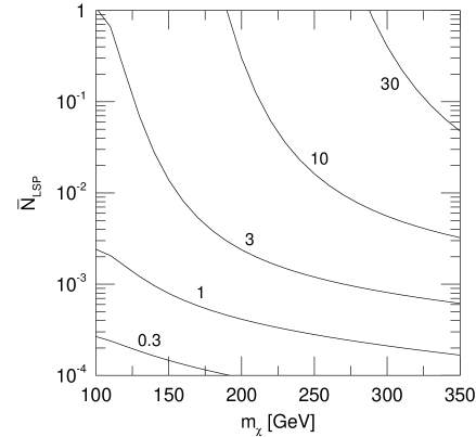
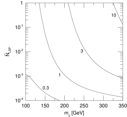
Figure 1: Contours of the constant $\Omega_{\chi}h^{2}$ on $m_{\chi}$ vs. $\bar{N}_{\rm LSP}$ plane. Numbers in the figure are $\Omega_{\chi}h^{2}$. Here, we take $\Lambda_{\rm eff}=M_{*}$ and $m_{\phi}=100~{}\mbox{TeV}$.

Figure 2: Same as Fig. 2, except $m_{\phi}=300~{}\mbox{TeV}$.

In Figs. 2 and 2, we plot the constant $\Omega_{\chi}h^{2}$ contour as a function of $m_{\chi}$ and  $\bar{N}_{\rm LSP}$ for $m_{\phi}=100~{}\mbox{TeV}$ and 300 TeV respectively. As we can see, for $\bar{N}_{\rm LSP}\sim 1$, $\Omega_{\chi}h^{2}$ is almost independent of $\bar{N}_{\rm LSP}$ since the pair annihilation is important in this region. (See Eq. (2.9).) However, for smaller $\bar{N}_{\rm LSP}$, the pair annihilation process becomes ineffective and $\Omega_{\chi}h^{2}$ becomes sensitive to $\bar{N}_{\rm LSP}$. (See Eq. (2.11).)

With the natural value of $\Lambda_{\rm eff}\sim M_{*}$, $\Omega_{\chi}h^{2}$ can be 0.1 $-$ 10, which is smaller than the result of the conventional calculation with the Bino LSP. In the AMSB, the Wino is the LSP, and hence the pair annihilation among the LSP’s is more enhanced than the Bino LSP case. Furthermore, the LSP density can be significantly suppressed if $\bar{N}_{\rm LSP}\ll 1$. (Notice that the second effect has not been considered before, and it can be important even in the Bino LSP case.) Because of these two reasons, the AMSB scenario realizes a smaller mass density of LSP’s from moduli decay. In particular, $\Omega_{\chi}h^{2}$ can be 0.1 $-$ 1 almost irrespective of the mass of the LSP for $\bar{N}_{\rm LSP}\sim 10^{-3}-10^{-4}$. In this case, we can avoid the problem of overclosing the Universe. Furthermore, even with $\bar{N}_{\rm LSP}\sim 1$, $\Omega_{\chi}h^{2}\sim O(1)$ if the Wino mass is less than about 200 GeV. So not only do we avoid the overproduction of Binos which is part of the cosmological moduli problem, but we actually see the the Wino is an excellent dark matter candidate.

The success of this scenario depends on the precise structure of the operators through which the moduli decay. The possible operators are listed in Appendix A. If the moduli are lighter than twice the gravitino mass, the operator (A.4) should be the most important. The operator (A.1) might also be important; however its coefficient is very likely loop-suppressed. In either case, we would expect $\bar{N}_{\rm LSP}\sim 10^{-3}-10^{-4}$, which is optimal for obtaining critical density for a large range of Wino mass. However, if $F_{\phi}$ is large, both operators (A.1) and (A.4) would have small coefficients in order to avoid too large a gaugino mass and $\mu$-parameter in the sequestered sector scenario. In this case, the moduli must decay into gravitino pairs through the operator (A.8). This would give a sufficiently high reheating temperature to avoid the first of the cosmological moduli problems, but requires a small Wino mass to obtain critical density (and not more) for the relic Winos. In this case, one requires slightly heavier moduli fields.

Finally, let us briefly discuss gravitino cosmology in the AMSB scenario. In the gravity-mediated SUSY breaking scenario, it is well known that a gravitino much lighter than ${\rm 10~{}TeV}$ is problematic [16]. In particular, the gravitinos are produced in the early Universe through scattering processes, and their decay can spoil the great success of the standard BBN scenario if $m_{3/2}\ll{\rm 10~{}TeV}$ [17]. Furthermore, the LSP may be overproduced via the decay of the gravitino. However, in the sequestered sector case, these problems may be avoided since the gravitino behaves almost like the modulus field. In the sequestered sector scenario, the gravitino mass can be so large that the decay happens before BBN starts. Furthermore, the LSP is produced by the decay of the gravitino with $\bar{N}_{\rm LSP}\simeq 1$, but the density of the LSP may be reduced by pair annihilation. The only difference is that the primordial number density of the gravitino is determined by the reheating temperature just after the primordial inflation, which we call $T_{\rm R}^{\rm(inf)}$. If we can neglect the pair annihilation of the produced LSP, the cosmological abundance of the LSP is proportional to the primordial abundance of the gravitino. In this case, if there is no effect from the modulus field, the mass density of the LSP is given by

$$\frac{\rho^{({\rm grav})}_{\chi}}{s}\simeq 1.4\times 10^{-9}\times\left(\frac{m_{\chi}}{100~{}\mbox{GeV}}\right)\left(\frac{T_{\rm R}^{\rm(inf)}}{10^{11}~{}\mbox{GeV}}\right),$$ (2.14)

where we used the gravitino abundance given in Ref. [18]. However, once the number density becomes large enough, the pair annihilation becomes effective and the above formula is not valid any more. In this case, it is relevant to use $\rho^{({\rm ann})}_{\chi}/s$ given in Eq. (2.9), since this is the maximally allowed mass density. (For the gravitino case, in Eq. (2.9), $\Lambda_{\rm eff}\sim M_{*}$ and $m_{\phi}=m_{3/2}$.) Therefore, the mass density of the LSP in this case is estimated as

$$\frac{\rho_{\chi}}{s}\sim\mbox{min}\left(\frac{\rho^{({\rm grav})}_{\chi}}{s},\frac{\rho^{({\rm ann})}_{\chi}}{s}\right).$$ (2.15)

When $T_{\rm R}^{\rm(inf)}\mathop{}_{\textstyle\sim}^{\textstyle>}10^{11}-10^{12}~{}{\rm GeV}$, the pair annihilation is effective and the mass density of the LSP becomes insensitive to $T_{\rm R}^{\rm(inf)}$. In particular, if $m_{\chi}\sim{\rm 100~{}GeV}$, $\Omega_{\chi}$ is always $O(1)$ for high enough $T_{\rm R}^{\rm(inf)}$, and the Wino-like LSP can be a candidate for CDM. If $m_{\chi}\gg{\rm 100~{}GeV}$, $T_{\rm R}^{\rm(inf)}$ should be tuned to be $\sim 10^{11}~{}{\rm GeV}$ to have $\Omega_{\chi}\sim 1$. Of course, if both the modulus field and the gravitino exist in the early Universe, primordial gravitinos can be diluted by the decay of the modulus field. In this case, the mass density of the LSP produced by the gravitino decay is negligible. The gravitino cosmology is also discussed in Ref. [13], but the authors neglected the effect of the pair annihilation of the LSP’s. As a result, they claimed that $T_{\rm R}^{\rm(inf)}\sim{\rm 10^{11}~{}GeV}$ is necessary to realize the Wino CDM. Based on Eq. (2.14), they also derived an upper bound on the reheating temperature of $T_{\rm R}^{\rm(inf)}\mathop{}_{\textstyle\sim}^{\textstyle<}{\rm 10^{11}~{}GeV}$ in order not to overclose the Universe. However, these arguments are modified as above once we include the effect of pair annihilation.

Since the decay of the modulus field produces a large entropy, one may worry about the dilution of the baryon asymmetry of the Universe in our scenario. It is true that the dilution factor due to the modulus decay can be as large as $\sim 10^{13}$, and hence large primordial baryon asymmetry is required. However, this is not necessarily a problem. For example, the Affleck-Dine baryogenesis [19] can provide enough baryon number asymmetry even with such a large dilution factor [4].

In summary, the mass density of the LSP produced by the decay of the moduli fields can be sufficiently suppressed in the Wino-like LSP case, and the AMSB scenario provides an interesting solution to the cosmological moduli problem. Furthermore, in this case, the Wino-like LSP is a natural candidate for CDM. In the next section, we will see this is a very advantageous situation from the point of view of dark matter detection.

3 Detecting Wino CDM

As we have seen, the Wino LSP is a promising candidate for cold dark matter. It comes out quite naturally from the parameters of the sequestered sector scenario. In this section, we consider the possibility of dark matter detection with Wino dark matter.

We first discuss the CDM search with Ge detectors. If the LSP is the dominant component of the mass density of the halo, we may observe the energy deposit due to the LSP-nucleus scattering in a Ge detector. In the sequestered sector scenario, squark masses are calculable and are generally quite heavy. Therefore, the scattering processes mediated by the squark exchange are suppressed.

However, the LSP $\chi$ also couples to the Higgs bosons as

$${\cal L}_{h\chi\chi}=y_{h\chi\chi}h\bar{\chi}\chi+y_{H\chi\chi}H\bar{\chi}\chi,$$ (3.1)

where $h$ and $H$ are the light and heavy CP even Higgses, respectively. Therefore, the LSP interacts with nuclei by exchanging the Higgs bosons. As we will see, this effect is important, and the detection rate in the Ge detector can be as large as $\sim 0.1-0.01$ event/kg/day which should be within the reach of the future detection of the CDM [20].

The above Yukawa coupling constants, $y_{h\chi\chi}$ and $y_{H\chi\chi}$, arise from the mixings between the Wino and Higgsinos. These mixings are from the off-diagonal elements in the neutralino mass matrix, which is given by

$${\cal M}=\left(\begin{array}[]{cccc}m_{\rm G1}&0&-m_{W}\cos\beta\tan\theta_{\rm W}&m_{W}\sin\beta\tan\theta_{\rm W}\\ 0&m_{\rm G2}&m_{W}\cos\beta&-m_{W}\sin\beta\\ -m_{W}\cos\beta\tan\theta_{\rm W}&m_{W}\cos\beta&0&-\mu\\ m_{W}\sin\beta\tan\theta_{\rm W}&-m_{W}\sin\beta&-\mu&0\end{array}\right),$$ (3.6)

in the basis $(i\tilde{B},i\tilde{W}^{0},\tilde{H}^{0}_{1},\tilde{H}^{0}_{2})$. Here, $m_{\rm G1}$ and $m_{\rm G2}$ are the gaugino masses for the gauginos associated with the U(1)_Y and SU(2)_L gauge groups respectively, $\mu$ is the supersymmetric Higgs mass, $\tan\beta$ is the ratio of Higgs VEVs, and $\theta_{\rm W}$ is the Weinberg angle. In the AMSB scenario, $m_{\rm G1}$ and $m_{\rm G2}$ are related by $m_{\rm G1}\simeq 3m_{\rm G2}$, which we now assume. The above mass matrix can be diagonalized by using a unitary matrix, which we call $U$. With this unitary matrix, the mass of the LSP is given by $m_{\chi}=|(U^{\dagger}{\cal M}U)_{11}|$, for example.

The Yukawa coupling constants are given by

$$y_{h\chi\chi} = -\frac{1}{2}g_{2}U_{21}(U_{31}\cos\beta-U_{41}\sin\beta),$$ (3.7)

$$y_{H\chi\chi} = -\frac{1}{2}g_{2}U_{21}(U_{31}\sin\beta+U_{41}\cos\beta).$$ (3.8)

Here, we neglect the difference between the neutral CP even Higgs mixing angle and the angle $\beta$. In the decoupling limit (i.e., $m_{h}\ll m_{H}$), this difference is sufficiently small. When $|\mu|$ and $|m_{\rm G2}|$ are much larger than $m_{W}$, the LSP is mostly the Wino and $U_{21}\simeq 1$. Other smaller elements are given by

$$U_{11}\simeq 0,~{}~{}~{}U_{31}\simeq-\frac{m_{W}(m_{\rm G2}\cos\beta-\mu\sin\beta)}{\mu^{2}-m_{\rm G2}^{2}},~{}~{}~{}U_{41}\simeq\frac{m_{W}(m_{\rm G2}\sin\beta+\mu\cos\beta)}{\mu^{2}-m_{\rm G2}^{2}},$$ (3.9)

and in the same limit, $y_{h\chi\chi}$ and $y_{H\chi\chi}$ are given by

$$y_{h\chi\chi} \simeq \frac{g_{2}m_{W}(m_{\rm G2}+\mu\sin 2\beta)}{2(\mu^{2}-m_{G2}^{2})},$$ (3.10)

$$y_{H\chi\chi} \simeq -\frac{g_{2}m_{W}\mu\cos 2\beta}{2(\mu^{2}-m_{G2}^{2})}.$$ (3.11)

As one can see, the coupling of the light Higgs is sensitive to the relative sign of $m_{\rm G2}$ and $\mu$; $y_{h\chi\chi}$ is enhanced if $\mu/m_{\rm G2}$ is positive. Furthermore, as the ratio $|\mu/m_{\rm G2}|$ becomes larger, the Higgsino component of the LSP becomes smaller. As a result, the $h\chi\chi$ and $H\chi\chi$ interactions are suppressed. In the Bino LSP case, $y_{h\chi\chi}$ and $y_{H\chi\chi}$ are given by similar expressions with $g_{2}m_{W}$ being replaced by $g_{1}m_{W}\tan\theta_{\rm W}$. Therefore, the Wino LSP has stronger couplings to the Higgs boson than the Bino, which enhances the detection cross section.

The interaction between the Higgs bosons and a nucleus are discussed in Ref. [21]. Since we are interested in a scattering process with small recoil energy, the nucleus can be approximately regarded as an elementary particle with mass $m_{N}$. Furthermore, since $m_{N}$ is dynamically generated through QCD effects, $m_{N}$ is proportional to the QCD scale $\Lambda_{\rm QCD}$. On the other hand, $\Lambda_{\rm QCD}$ is sensitive to the fluctuation of the Higgs fields through the heavy quark mass dependence of $\Lambda_{\rm QCD}$. By using these facts, we can relate the Higgs VEV dependence of the QCD scale to the Higgs-nucleus coupling constants. The interaction terms of the Higgs bosons with the nucleus $N$ are derived as [21]

$${\cal L}_{\rm int}=\frac{\partial{\cal L}_{\rm mass}}{\partial m_{N}}(y_{hNN}h+y_{HNN}H),$$ (3.12)

where ${\cal L}_{\rm mass}$ is the mass term for the nucleus $N$ in the effective theory. We consider the case with Ge detector, and we will use the formula for $N={\rm{}^{76}Ge}$. The “effective” coupling constants for the Higgs interactions are given by

$$y_{hNN} = -\frac{2}{9}\frac{m_{N}}{v},$$ (3.13)

$$y_{HNN} = -\frac{2}{27}\frac{m_{N}}{v}(\tan\beta-2\cot\beta),$$ (3.14)

with $v\simeq{\rm 246~{}GeV}$. As one can see in Eq. (3.14), the interaction of the heavy Higgs becomes stronger in the large $\tan\beta$ case, and the heavy Higgs exchange diagram may enhance the detection rate.

With the above coupling constants, the total cross section for the scattering process $\chi N\rightarrow\chi N$ is given by

$$\sigma_{\rm scatt}=\frac{4}{\pi}\left(\frac{y_{hNN}y_{h\chi\chi}}{m_{h}^{2}}+\frac{y_{HNN}y_{H\chi\chi}}{m_{H}^{2}}\right)^{2}\frac{m_{N}^{2}m_{\chi}^{2}}{(m_{N}+m_{\chi})^{2}},$$ (3.15)

where $m_{h}$ and $m_{H}$ are the masses of $h$ and $H$, respectively. Assuming that the CDMs are virialized in the halo, we obtain the detection rate

$$R=\frac{2}{\sqrt{3\pi}}\frac{\rho_{\chi}^{\rm(halo)}\bar{v}_{\chi}\sigma_{\rm scatt}}{m_{N}m_{\chi}}\exp\left(-\frac{3(m_{N}+m_{\chi})^{2}E_{\rm thr}}{4m_{N}m_{\chi}^{2}\bar{v}_{\chi}^{2}}\right),$$ (3.16)

where $\rho_{\chi}^{\rm(halo)}$ is the mass density of the LSP in the halo, $E_{\rm thr}$ is the threshold energy of the detector, and $\bar{v}_{\chi}$ is the averaged velocity of the LSP in the halo.

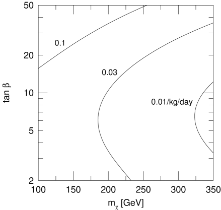
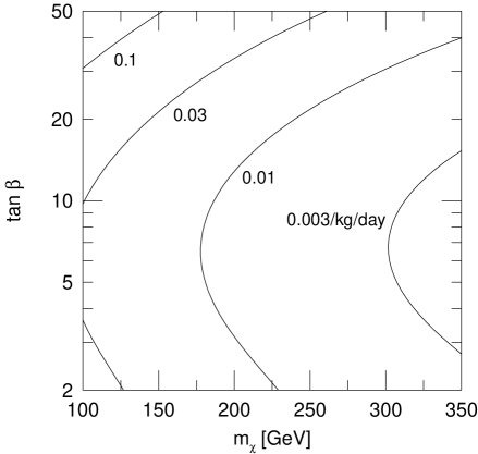
Figure 3: Contours of the constant detection rate $R$ in ⁷⁶Ge detector on $m_{\chi}$ vs. $\tan\beta$ plane. We take the parameters of $\mu=2m_{\rm G2}$, $m_{h}={\rm 100~{}GeV}$, $m_{H}={\rm 300~{}GeV}$, $E_{\rm thr}={\rm 2~{}keV}$, $\bar{v}_{\chi}={\rm 320~{}km/sec}$ and $\rho_{\chi}^{\rm(halo)}={\rm 0.3~{}GeV/cm^{3}}$.

Figure 4: Same as Fig. 4, except $\mu=3m_{\rm G2}$.

In Figs. 4 and 4, we show the expected detection rate of the Wino CDM in a ⁷⁶Ge detector for $\mu=2m_{\rm G2}$ and $\mu=3m_{\rm G2}$, respectively. In our calculation, we used the Higgs masses $m_{h}={\rm 100~{}GeV}$ and $m_{H}={\rm 300~{}GeV}$. The other parameters are taken to be $E_{\rm thr}={\rm 2~{}keV}$, $\bar{v}_{\chi}={\rm 320~{}km/sec}$, and $\rho_{\chi}^{\rm(halo)}={\rm 0.3~{}GeV/cm^{3}}$.

The behavior of Figs. 4 and 4 can be understood as follows. In the small $\tan\beta$ region, the scattering is dominated by the light Higgs exchange diagram. In this case, the detection rate $R$ decreases as $\tan\beta$ increase since $y_{h\chi\chi}$ is more suppressed for large $\tan\beta$ (if $\mu/m_{\rm G2}>0$). On the other hand, for the large $\tan\beta$ region, heavy Higgs exchange is the dominant contribution. Since the $HNN$ coupling $y_{HNN}$ is proportional to $\tan\beta$, $R$ is more enhanced for larger $\tan\beta$. Furthermore, $R$ decreases as $m_{\chi}\simeq|m_{\rm G2}|$ or $|\mu|$ increases, since the Wino-Higgsino mixing is more suppressed in this limit.

We can see that the detection rate of order 0.1 $-$ 0.01 event/kg/day is possible in a Ge detector, which is within the reach of the on-going CDM searches [20]. The detection rate is considerably larger than the conventional Bino CDM case. This is because the couplings $y_{h\chi\chi}$ and $y_{H\chi\chi}$ are (approximately) proportional to $g_{2}^{2}$ for the Wino LSP, instead of $g_{1}^{2}$ for the Bino LSP. Indeed, in the minimal supergravity model with the Bino LSP, the detection rate is typically $O(10^{-3}~{}{\rm event/kg/day})$ or less [22], which is an order of magnitude smaller than what is detectable. Therefore, the Wino CDM has more chance to be detected in a Ge detector. Of course, the detection rate given in Eq. (3.16) is sensitive to the model parameters. For example, the discovery of the signal will be difficult if $|\mu|\gg|m_{\rm G2}|$. Furthermore, in the large $\tan\beta$ region, $R\propto m_{H}^{-4}$ and the detection rate decreases as $m_{H}$ increases. However, too large $\mu$ and too heavy Higgs are not preferred from the naturalness point of view. Therefore, in a significant fraction of the parameter space of the AMSB scenario, the Wino CDM should be detectable.

For $\mu/m_{\rm G2}<0$, $y_{h\chi\chi}$ is suppressed because of the cancellation, as shown in Eq. (3.10). Therefore, in this case, the detection of the Wino CDM is difficult for small $\tan\beta$. On the other hand, for large $\tan\beta$, the detection rate is less sensitive to the relative sign between $\mu$ and $m_{\rm G2}$, and detection might be possible.

There is an alternative means to search for dark matter, which is to look for the energetic neutrinos produced by the annihilation of the Wino LSP’s captured in the center of the sun and/or earth [23]. Such a high energy neutrino can be converted to a high energy muon which can be observed as an upward going muon in Čerenkov detectors. Using the conversion factors given in Ref. [24], we find that an LSP with $R\sim 0.1-0.01~{}{\rm event/kg/day}$ has the event rate for indirect detection in the Čerenkov detectors of $\Gamma_{\rm ID}\sim 10-1~{}{\rm event/m^{2}/yr}$. This is less sensitive than the direct detection in a Ge detector [24].

It might be that the most promising method for searching for dark matter is to look for anti-matter, either anti-protons [25] or positrons [26, 27], produced by the pair annihilation of the LSP in our galaxy. The pair annihilation rate $\langle v_{\rm rel}\sigma\rangle$ for the Wino LSP is given in Eq. (2.4), and numerically is given by $3.8\times 10^{-24}~{}{\rm cm^{3}/sec}$ (for $m_{\chi}={\rm 100~{}GeV}$) $-$ $0.9\times 10^{-24}~{}{\rm cm^{3}/sec}$ (for $m_{\chi}={\rm 300~{}GeV}$). Unlike standard SUSY dark matter, this rate is very large, and we expect a high flux of anti-particles. Furthermore, there are several on-going projects for measuring the anti-matter flux in the cosmic ray. In particular, a very accurate measurement is expected by the AMS experiment [28], which is a search for anti-matters with “Alpha Magnetic Spectrometer” on the space shuttle and on the international space station. Since the experiment is not affected by the atmosphere, AMS will greatly improve the measurements of the anti-matter fluxes in the cosmic ray.

A recent calculation of the anti-proton flux $\Phi_{\bar{p}}$ can be found in Ref. [29] where the flux from an LSP which dominantly annihilates into $W$-boson pair is presented (see Example No. 4 in Ref. [29]). Since $\Phi_{\bar{p}}$ from the LSP annihilation is proportional to $\langle v_{\rm rel}\sigma\rangle\times(\rho_{\chi}^{\rm(halo)}/m_{\chi})^{2}$, we estimate the anti-proton flux by rescaling the result given in Ref. [29]. Adopting the canonical astrophysical parameters of Ref. [29], we find $\Phi_{\bar{p}}$ to be $0.46~{}{\rm m^{-2}sec^{-1}sr^{-1}GeV^{-1}}$ (for $m_{\chi}={\rm 100~{}GeV}$) $-$ $0.012~{}{\rm m^{-2}sec^{-1}sr^{-1}GeV^{-1}}$ (for $m_{\chi}={\rm 300~{}GeV}$). Experimentally, the anti-proton flux is already measured by the BESS experiment, and is given by $(1.36^{+0.86}_{-0.61})\times 10^{-2}~{}{\rm m^{-2}sec^{-1}sr^{-1}GeV^{-1}}$ [30]. As a result, a naive comparison of our estimate with the measured flux would already imply the constraint $m_{\chi}\mathop{}_{\textstyle\sim}^{\textstyle>}250~{}{\rm GeV}$. One should note, however, that the flux is proportional to ${\rho^{\rm(halo)}_{\chi}}^{2}$. Furthermore, if we change the model of the halo, it affects the propagation of the anti-proton and the flux can be reduced significantly [29]. Therefore, the theoretical result is very sensitive to astrophysics parameters, and we do not draw any strong conclusion here. It is unlikely that the situation for anti-protons will improve with the AMS experiment, since the anti-proton signal falls with higher energy faster than the background. However, the situation for positrons is very promising as we now discuss.

$m_{\chi}$	$\Phi_{e^{+}}/(\Phi_{e^{-}}+\Phi_{e^{+}})_{\rm Wino}$	$\Phi_{e^{+}}/(\Phi_{e^{-}}+\Phi_{e^{+}})_{\rm BG}$
100 GeV	0.15	0.032
300 GeV	0.049	0.026

Table 1: The positron fraction $\Phi_{e^{+}}/(\Phi_{e^{-}}+\Phi_{e^{+}})$ in the cosmic ray at the peak of the spectrum. The second column is the result with the Wino CDM. The third column is the background estimated from the conventional sources.

In Ref. [29], the positron flux, $\Phi_{e^{+}}$, is also presented. Rescaling the given result, we found that $\Phi_{e^{+}}$ from the Wino-like CDM is comparable to the currently measured flux by the HEAT experiment [31] even for $m_{\chi}\simeq{\rm 100~{}GeV}$. Therefore, we believe our scenario is not seriously constrained by the present data, but could give a very prominent signal in the future. One important point is that the positron spectrum from the Wino CDM is peaked at high energy ($\sim\frac{1}{2}m_{\chi}$) [26, 27], which can be a distinctive signature of the Wino annihilation in the halo. In order to study the significance of this signal, we rescaled the results given in Ref. [27] to obtain the positron fraction $\Phi_{e^{+}}/(\Phi_{e^{-}}+\Phi_{e^{+}})$ at the peak. The results are given in Table 1. As one can see, with the Wino CDM, the positron fraction can be about 5 $-$ 2 times larger than the background for $m_{\chi}={\rm 100-300~{}GeV}$. A measurement of the positron fraction has recently performed at lower energies by AMS who will also do very precise measurement at higher energies in the future. Since the signal can be peaked at higher energy, this should be an excellent way to search for Wino CDM. The signal is much stronger for Wino CDM than the more frequently studied Bino dark matter, which would be undetectable. The distortion suggested here should provide strong evidence for the Wino CDM scenario.

4 Conclusion

In this paper, we discussed the cosmological moduli problem in the sequestered sector/AMSB scenario. In this scheme, the gravitino mass (corresponding to the moduli mass) is naturally 10 $-$ 100 TeV. As a result, cosmological moduli fields can decay before BBN starts. Furthermore, since the LSP is likely to be the Wino-like neutralino, the production of the LSP through moduli decay can be suppressed and the Universe should not be overclosed, contrary to the case of the Bino-like LSP. Moreover, the mass density of the Wino-like LSP can be naturally close to the critical density of the Universe, and hence the Wino is an interesting candidate for CDM. Furthermore, we have seen that if the halo density is dominated by the Wino CDM, the detection rate of the Wino CDM in Ge detector can be as large as $0.1-0.01$ event/kg/day, which is within the reach of the CDM search experiment, and furthermore, the positron signal in AMS should be measurable.

Appendix A Moduli Field Couplings

In this Appendix, we discuss the mass and couplings of the moduli fields.

We assume that a modulus field $\phi$ acquires its mass from SUSY breaking effects. Therefore, its mass is expected to be of the order of the gravitino mass $m_{3/2}\sim{\rm 10-100~{}TeV}$ [2]. Some non-perturbative effects may be able to give much larger masses to the moduli fields. Such a heavy modulus field is cosmologically safe since its lifetime can be much shorter than 1 sec.

It is also important to understand the relevant operators which contribute to the decay of $\phi$. By taking the minimal SUSY standard model (MSSM) as the low energy effective theory, the following operators can exist.

The modulus field can decay into a gauge field (and gaugino) through the operators:

$${\cal L}_{\rm G}=\int d^{2}\theta\frac{\lambda_{\rm G}}{M_{*}}\phi W^{\alpha}W_{\alpha}+\mbox{h.c.},$$ (A.1)

where $\lambda_{\rm G}$ is a constant to parameterize the strength of this interaction. When the gaugino mass $m_{\tilde{G}}$ is much smaller than $m_{\phi}$, the branching ratio for the decay into the gaugino pair receives chirality suppression [10]. As a result, the (partial) decay width and $\bar{N}_{\rm LSP}$ is given by

$$\Gamma_{\rm G} = \frac{N_{\rm f}\lambda_{\rm G}^{2}}{8\pi}\frac{m_{\phi}^{3}}{M_{*}^{2}},$$ (A.2)

$$\bar{N}_{\rm LSP} \sim O(m_{\tilde{G}}^{2}/m_{\phi}^{2}),$$ (A.3)

where $N_{\rm f}$ is the number of the possible final states. (For example, $N_{\rm f}=N^{2}-1$ for an SU($N$) gauge group.) One should note that this operator also contributes to the gaugino mass if the $\phi$ field participates in SUSY breaking. So either $\lambda_{G}$ is suppressed or $F_{\phi}$ is in order to maintain the anomaly-mediated predictions.

In the MSSM, the following operator is also allowed:

$${\cal L}_{\rm H}=\int d^{4}\theta\frac{\lambda_{\rm H}}{M_{*}}\phi H_{1}^{*}H_{2}^{*}+\mbox{h.c.},$$ (A.4)

where $H_{1}$ and $H_{2}$ are the down-type and up-type Higgses, respectively. With this operator, the modulus field can decay into a Higgs boson pair, and the decay width for this process is

$$\Gamma_{\rm H}=\frac{\lambda_{\rm H}^{2}}{8\pi}\frac{m_{\phi}^{3}}{M_{*}^{2}}.$$ (A.5)

Notice that the Higgsino cannot be produced from this operator, and hence $\bar{N}_{\rm LSP}=0$ for this process. This operator is also dangerous if $F_{\phi}$ is maximal since it generates too large $\mu$-parameter.

One can also write down the following operator:

$${\cal L}_{\rm Q^{*}Q}=\int d^{4}\theta\frac{\lambda_{\rm Q^{*}Q}}{M_{*}}\phi Q^{*}Q+\mbox{h.c.}=\frac{\lambda_{\rm Q^{*}Q}}{M_{*}}\phi(\partial^{2}\tilde{Q}^{*})\tilde{Q}+\cdots,$$ (A.6)

where $Q$ is general chiral superfields in the MSSM and $\tilde{Q}$ is its scalar component. As suggested from the structure of the operator, the decay rate is given by

$$\Gamma_{Q^{*}Q}\sim O\left(\frac{\lambda_{\rm Q^{*}Q}^{2}}{4\pi}\frac{m_{\tilde{Q}}^{4}}{m_{\phi}^{4}}\frac{m_{\phi}^{3}}{M_{*}^{2}}\right),$$ (A.7)

where $m_{\tilde{Q}}$ is the soft SUSY breaking mass for $\tilde{Q}$. Therefore, the decay through this operator is suppressed by a factor of $O(m_{\tilde{Q}}^{4}/m_{\phi}^{4})$.

In supergravity, we also expect the following interaction:

$${\cal L}_{\psi}=-\frac{1}{M_{*}^{2}}e^{K/2}W\psi_{\mu}\sigma^{\mu\nu}\psi_{\nu}+\mbox{h.c.},$$ (A.8)

where $K$ and $W$ are the Kähler potential and superpotential, and $\psi_{\mu}$ is the gravitino field, respectively. If the decay $\phi\rightarrow\psi_{\mu}\psi_{\mu}$ is kinematically allowed, the effect of this operator can be important. In this case, $\phi$ decays into a gravitino pair; then the produced gravitino decays into the standard model particle and its superpartner through the supercurrent interaction. For this process, the effective decay width (i.e., the inverse of the time scale of this process) and $\bar{N}_{\rm LSP}$ are estimated as

$$\Gamma_{\psi} \sim O\left(\frac{1}{4\pi}\frac{m_{3/2}^{3}}{M_{*}^{2}}\right),$$ (A.9)

$$\bar{N}_{\rm LSP} \sim O(1).$$ (A.10)

There are also several operators that permit three-body decay. For example, a modulus field can couple to the Yukawa-type operator in the $F$-term like

$${\cal L}_{\rm Y}=\int d^{2}\theta\frac{\lambda_{\rm Y}}{M_{*}}\phi H_{2}t_{\rm R}^{\rm c}q_{\rm L}+\mbox{h.c.},$$ (A.11)

where $H_{2}$, $t_{\rm R}^{\rm c}$, and $q_{\rm L}$ are chiral superfields for up-type Higgs, right-handed top quark, and left-handed third generation quark doublet, respectively. With this operator, the decay rate is calculated as

$$\Gamma_{\rm Y}=\frac{3\lambda_{\rm Y}^{2}}{128\pi^{3}}\frac{m_{\phi}^{3}}{M_{*}^{2}}.$$ (A.12)

This is a three-body process, and hence the decay rate is more suppressed than those of the two-body processes. For this process, $\bar{N}_{\rm LSP}\sim O(1)$. One may also write down the scalar interaction of the form $\frac{m_{3/2}}{M_{*}}\phi H_{2}\tilde{t}_{\rm R}^{\rm c}\tilde{q}_{\rm L}$ arising from the supergravity effect. If the coefficient of this operator is $O(1)$, however, too large an $A$-parameter is generated with $\langle\phi\rangle\sim M_{*}$. Therefore, we assume this operator is somehow suppressed if $\langle\phi\rangle\sim M_{*}$.

So, to summarize, the moduli fields are expected to have a decay rate as large as that estimated on dimensional grounds. The operators that could lead to this decay rate are the operator given in Eq. (A.8) which leads to the decay to gravitinos (if kinematically permitted), the coupling to gauge pairs (A.1), and the coupling to Higgses (A.4). However, a large value for the last two couplings require a small value for $F_{\phi}$. The decay rate with no suppression factors is consistent with the requirements for avoiding the cosmological moduli problem.

The density of Wino dark matter depends on $\bar{N}_{\rm LSP}$. In general, $\bar{N}_{\rm LSP}$ is expected to be small. The precise value depends on the magnitude of the coupling of the associated operators, but values of order $10^{-4}-10^{-2}$ are expected. The exception to this small value is the operator that permits decay to gravitinos. If kinematically possible, this would permit large $\bar{N}_{\rm LSP}\sim 1$.

References

- [1] G.D. Coughlan, W. Fischler, E.W. Kolb, S. Raby and G.G. Ross, Phys. Lett. B131 (1983) 59; T. Banks, D.B. Kaplan and A.E. Nelson, Phys. Rev. D49 (1994) 779; T. Banks, M. Berkooz and P.J. Steinhardt, Phys. Rev. D52 (1995) 705.
- [2] B. de Carlos, J.A. Casas, F. Quevedo and E. Roulet, Phys. Lett. B318 (1993) 447.
- [3] J. Ellis, D.V. Nanopoulos and M. Quiros, Phys. Lett. B174 (1986) 176.
- [4] T. Moroi, M. Yamaguchi and T. Yanagida, Phys. Lett. B342 (1995) 105.
- [5] L. Randall and S. Thomas, Nucl. Phys. B449 (1995) 229.
- [6] M. Kawasaki, T. Moroi and T. Yanagida, Phys. Lett. B370 (1996) 52.
- [7] T. Nagano and M. Yamaguchi, Phys. Lett. B438 (1998) 267.
- [8] L. Randall and R. Sundrum, hep-th/9810155.
- [9] G. Giudice, M. Luty, H. Murayama and R. Rattazzi, JHEP 9812 (1998) 027.
- [10] M. Dine, L. Randall and S. Thomas, Phys. Rev. Lett. 75 (1995) 398.
- [11] D.H. Lyth and E.D. Stewart, Phys. Rev. Lett. 75 (1995) 201; Phys. Rev. D53 (1996) 1784.
- [12] J.L. Feng, T. Moroi, L. Randall, M. Strassler and S. Su, hep-ph/9904250.
- [13] T. Gherghetta, G.F. Giudice and J.D. Wells, hep-ph/9904378.
- [14] See, for example, E.W. Kolb and M.S. Turner, The Early Universe (Addison-Wesley, 1990).
- [15] M. Kawasaki, K. Kohri and N. Sugiyama, Phys. Rev. Lett. 82 (1999) 4168.
- [16] S. Weinberg, Phys. Rev. Lett. 48 (1982) 1303.
- [17] M.Y. Khlopov and A.D. Linde, Phys. Lett. B138 (1984) 265; J. Ellis, E. Kim and D.V. Nanopoulos, Phys. Lett. B145 (1984) 181.
- [18] M. Kawasaki and T. Moroi, Prog. Theor. Phys. 93 (1995) 879.
- [19] I. Affleck and M. Dine, Nucl. Phys. B249 (1985) 361.
- [20] See, for example, G. Jungman, M. Kamionkowski and K. Griest, Phys. Rept. 267 (1996) 195.
- [21] M.A. Shifman, A.I. Vainstein and V.I. Zakharov, Phys. Lett. B78 (1978) 443.
- [22] M. Drees and M.M. Nojiri, Phys. Rev. D48 (1993) 4483.
- [23] J. Silk, K. Olive and M. Srednicki, Phys. Rev. Lett. 55 (1985) 257; L.M. Krauss, M. Srednicki and F. Wilczek, Phys. Rev. D33 (1986) 2079; K. Freese, Phys. Lett. B167 (1986) 295.
- [24] M. Kamionkowski, K. Griest, G. Jungman and B. Sadoulet, Phys. Rev. Lett. 74 (1995) 5174.
- [25] J. Silk and M. Srednicki, Phys. Rev. Lett. 53 (1984) 624.
- [26] M.S. Turner and F. Wilczek, Phys. Rev. D42 (1990) 1001.
- [27] M. Kamionkowski and M.S. Turner, Phys. Rev. D43 (1991) 1774.
- [28] The AMS collaboration, http://hpl3tri1.cern.ch/.
- [29] L. Bergström, J. Edsjö and P. Ullio, astro-ph/9902012.
- [30] H. Matsunaga et al., Phys. Rev. Lett. 81 (1998) 4052.
- [31] S.W. Barwick et al., astro-ph/9712324.
- [32] S. Coutu et al., astro-ph/9902162.