CERN-TH/98-399, December 1998, hep-ph/9906476

A TWO-LOOP APPLICATION OF THE THRESHOLD EXPANSION: THE BOTTOM QUARK MASS FROM $b\bar{b}$ PRODUCTION

We use the threshold expansion and non-relativistic effective theory to determine the bottom quark mass from moments of the $b\bar{b}$ production cross section at next-to-next-to-leading order in the (resummed) perturbative expansion, and including a summation of logarithms. For the $\overline{\rm MS}$ mass $\overline{m}_{b}$, we find $\overline{m}_{b}(\overline{m}_{b})=(4.26\pm 0.12)\,$GeV.

1 Introduction

In this talk we report on a determination of the bottom quark mass at next-to-next-to-leading order (NNLO) based on dispersion relations for $e^{+}e^{-}\to b\bar{b}X$. This idea dates back to Ref. $\!{}^{{\bf?}}$ and relies on the relation

$$\frac{12\pi^{2}}{n!}\,\frac{d^{n}}{d(q^{2})^{n}}\,\Pi(q^{2})_{\big{|}q^{2}=0}=\int_{0}^{\infty}\frac{ds}{s^{n+1}}\,R_{b\bar{b}}(s),$$ (1)

between the two-point function of the bottom vector current and the inclusive bottom quark cross section mediated by a virtual photon, which is valid up to a small correction from $b\bar{b}$ radiation from light quarks. The left hand side can be computed in perturbation theory; the right hand side from data.

The parameters of the lowest $\Upsilon(nS)$ resonances are well-measured, but the continuum cross section above the threshold is not. Hence the experimental error of the right hand side decreases with increasing $n$, because higher moments weight lower $s$. When the integral over $s$ is saturated by the threshold region, the bottom quarks are non-relativistic, and $2m_{b}/\sqrt{n}$ and $m_{b}/n$ appear as new momentum scales in the problem, related to the typical momentum $m_{b}v$ and non-relativistic energy $m_{b}v^{2}$ of the bottom quarks, respectively. When $n$ is large enough such that $v\sim\alpha_{s}$, ordinary perturbation theory breaks down, because there are terms of the form $(\alpha_{s}/v)^{k}$ to all orders in perturbation theory. Even when $v$ is only small, but not as small as $\alpha_{s}$, one may want to resum those enhanced terms systematically.

Defining $v=(1-4m_{b}^{2}/s)^{1/2}$, where $m_{b}$ is the $b$ quark pole mass, the cross section $e^{+}e^{-}\to b\bar{b}X$ for $s\approx 4m_{b}^{2}$ can be expanded in a double series in $\alpha_{s}$ and $v$:

$$R_{b\bar{b}}=v\sum_{k=0}\,\sum_{l=-k}c_{kl}\,\alpha_{s}^{k}\,v^{l}\times\,\mbox{logs of}\,\,v.$$ (2)

In the resummed perturbative expansion, a N^pLO calculation has to account for all terms with $k+l\leq p$. Such a rearranged expansion has first been considered in this context in Ref. $\!{}^{{\bf?}}$ to LO accuracy and in Ref. $\!{}^{{\bf?}}$ to NLO accuracy. The step to NNLO accuracy implies new difficulties, because at this order the naive relativistic or non-relativistic approximations lead separately to divergent integrals. One has to be more precise about factorizing the two momentum regimes.

Powers of $v$ in (2) arise from ratios of momentum scales. We have to disentangle the contributions from the different scales in order to be sure that for a high-order loop graph, which cannot be calculated exactly, we have taken into account all terms with $k+l\leq 2$. In Ref. $\!{}^{{\bf?}}$ we described how to expand a Feynman integral in $v$ to any given order, without calculating the exact result. The expansion procedure is based on decomposing the loop integral into contributions from different loop momentum regions and has a transparent interpretation in terms of effective theories. The present application, the perturbative calculation of $R_{b\bar{b}}$ in the threshold region, has much in common with a QED bound state calculation done with non-relativistic QED $\!{}^{{\bf?},{\bf?}}$. The main difference is that we perform factorization in dimensional regularization, rather than using momentum space cut-offs and a photon mass as infrared regulator, and take advantage of the fact that scaleless integrals vanish in dimensional regularization. The absence of any explicit cut-off scale leads to a homogeneous expansion in $v$, manifest power counting and makes analytic calculations much easier at two loops. The unfamiliar dimensional renormalization of the Schrödinger problem is a negligible price to pay in comparison to these advantages, because it is not necessary to obtain the Green function exactly in $d$ dimensions.

In the following we summarize the calculation of $e^{+}e^{-}\to b\bar{b}X$ at NNLO using these methods $\!{}^{{\bf?},{\bf?}}$ and we determine the bottom quark mass by calculating the moment integral (1). In addition to the NNLO terms in the sense of (2), we also sum all logarithms of $v$ of the form $(\alpha_{s}\ln v)^{k}$ and $\alpha_{s}\,(\alpha_{s}\ln v)^{k}$. A subset of NNLO logarithms of the form $\alpha_{s}^{2}\,(\alpha_{s}\ln v)^{k}$ can easily be summed as well, but a complete summation requires another difficult calculation to be done. This write-up concentrates on necessary formulae. A more general perspective on the problem, and a more complete list of references related to the subject can be found in Ref. $\!{}^{{\bf?}}$. While we were preparing this work, other NNLO calculations appeared $\!{}^{{\bf?},{\bf?},{\bf?}}$. A brief comparison with these results is given at the end.

2 Heavy quark production cross section near threshold

2.1 Classification of momentum regions

The expansion (2) can be constructed by decomposing each Feynman integral that contributes to the vacuum polarization $\Pi(q^{2})$ into contributions from the following momentum regions $\!{}^{{\bf?}}$:

hard (h): $$l_{0}\sim m_{b},\,\,\vec{l}\sim m_{b},$$

soft (s): $$l_{0}\sim m_{b}v,\,\,\vec{l}\sim m_{b}v,$$

potential (p): $$l_{0}\sim m_{b}v^{2},\,\,\vec{l}\sim m_{b}v,$$ (3)

ultrasoft (us): $$l_{0}\sim m_{b}v^{2},\,\,\vec{l}\sim m_{b}v^{2},$$

assuming a frame where $\vec{q}=0$. In dimensional regularization, the factorization of the different momentum regions is achieved by appropriate expansions of the Feynman integrands, without the need for explicit cut-offs, so that one can integrate over the whole integration domain in each region. As a consequence of this expansion, all terms have a definite homogeneous scaling behaviour in $v$.

In the following, we integrate out first the hard, relativistic modes. This defines the NRQCD Lagrangian in dimensional regularization. In a second step, we also integrate out soft modes and potential gluon modes to arrive at another effective theory, ‘potential NRQCD’ (PNRQCD), the QCD analogue of PNRQED, introduced in Ref. $\!{}^{{\bf?}}$. The final result is obtained by computing the vacuum polarization in PNRQCD perturbation theory, with the Coulomb interaction treated non-perturbatively.

2.2 Relativistic corrections

At tree-level relativistic corrections arise from the anti-particle pole of the heavy quark propagator and the anti-particle components of the heavy quark four-spinor field. Beyond tree level, the hard loop momentum regions induce further terms in the non-relativistic effective theory.

The heavy quark current correlation function $\Pi(q^{2})$ contains 1PI, hard subgraphs which (a) do not connect to the virtual photon vertex, (b) connect to one of the virtual photon vertices and (c) connect to both virtual photon vertices. The last possibility is of no interest, since it cannot contribute to the discontinuity of $\Pi(q^{2})$ and hence is irrelevant for the computation of (1).

Accounting for the hard subgraphs (a) leads to the familiar NRQCD Lagrangian $\!{}^{{\bf?},{\bf?}}$. At NNLO, the following terms are needed:

$${\cal L}_{\rm NRQCD} = \psi^{\dagger}\left(iD^{0}+\frac{\vec{D}^{2}}{2m_{b}}\right)\psi+\frac{1}{8m_{b}^{3}}\,\psi^{\dagger}\vec{D}^{4}\psi-\frac{d_{1}\,g_{s}}{2m_{b}}\,\psi^{\dagger}\vec{\sigma}\cdot\vec{B}\psi$$ (4)

$$+\,\frac{d_{2}\,g_{s}}{8m_{b}^{2}}\,\psi^{\dagger}\left(\vec{D}\cdot\vec{E}-\vec{E}\cdot\vec{D}\right)\psi+\frac{d_{3}\,ig_{s}}{8m_{b}^{2}}\,\psi^{\dagger}\vec{\sigma}\cdot\left(\vec{D}\times\vec{E}-\vec{E}\times\vec{D}\right)\psi$$

$$+\,\,\mbox{antiquark terms}\,+{\cal L}_{\rm light}.$$

Since we work in dimensional regularization, $\epsilon_{ijk}$ should be defined carefully. As long as we are only interested in $\Pi(q^{2})$, we can avoid the problem by writing the Lagrangian in terms of anti-commutators of Pauli-matrices. Hence $\vec{\sigma}\cdot\vec{B}$ must be interpreted as $i/4\,[\sigma^{i},\sigma^{j}]\,G^{ij}$. A similar interpretation holds for the spin-orbit interaction. The scaling of the interaction terms relative to $\psi^{\dagger}iD^{0}\psi$ depends on whether the quark and gluons fields are considered as soft, potential or (in the case of gluons) ultrasoft. For potential quarks, $\vec{D}^{2}/(2m_{b})$ is a leading order term, so its coefficient would be needed to order $\alpha_{s}^{2}$. However, since the coefficient is 1 to all orders in PT, there is nothing to calculate. The chromomagnetic interaction is suppressed by only one power of $v$ for a soft gluon and by two powers of $v$ for an ultrasoft gluon. However, since one needs at least two chromomagnetic insertions to obtain a non-vanishing contribution to $\Pi(q^{2})$, it is sufficient to know $d_{1}$ at tree level. Since, for the time being, we sum logarithms of $v$ only at NLO and not at NNLO, we have $d_{1}=d_{2}=d_{3}=1.$

Accounting for the hard subgraphs (b) leads to the effective non-relativistic $\gamma^{\star}b\bar{b}$ coupling

$$\bar{Q}\gamma^{i}Q = c_{1}\,\psi^{\dagger}\sigma^{i}\chi-\frac{c_{2}}{6m_{b}^{2}}\,\psi^{\dagger}\sigma^{i}(i\vec{D})^{2}\chi+\ldots,$$ (5)

where the ellipsis refers to terms not needed for $\Pi(q^{2})$ and at NNLO. At NNLO, we can use $c_{2}=1$, while $c_{1}$ is needed at order $\alpha_{s}^{2}$. The required matching calculation has been done in Refs. $\!{}^{{\bf?},{\bf?}}$. The result is

$$c_{1}(\mu)=1+\left[c_{1}^{(1)}\frac{\alpha_{s}(m_{b})}{4\pi}+\delta_{1}\left(\frac{\alpha_{s}(m_{b})}{4\pi}-\frac{\alpha_{s}(\mu)}{4\pi}\right)\right]+c_{1}^{(2)}\left(\frac{\alpha_{s}(m_{b})}{4\pi}\right)^{\!2},$$ (6)

where

$$c_{1}^{(1)}=-\frac{32}{3},\qquad\delta_{1}=-\frac{1120\pi^{2}}{54b_{0}},$$

$$c_{1}^{(2)}=-\frac{712}{27}-\frac{2044\pi^{2}}{81}-\frac{224\pi^{2}}{9}\ln 2-\frac{2000\zeta(3)}{9}+\frac{176}{27}\,n_{f}$$ (7)

and $b_{0}=11-2n_{f}/3$. The term proportional to $\delta_{1}$ sums all next-to-leading logarithms of the form $\alpha_{s}(\alpha_{s}\ln v)^{k}$. There are no leading logarithms and this term is the only source of next-to-leading logarithms in the problem.

2.3 Instantaneous interactions

The loop diagrams constructed from the NRQCD Lagrangian contain soft, potential and ultrasoft modes. We now integrate out the soft modes and potential gluons. As discussed in $\!{}^{{\bf?},{\bf?}}$, these modes give rise to instantaneous interactions. At NNLO, it is sufficient to match the (on-shell) quark-antiquark scattering amplitude to the required order. We do this order by order in $\alpha_{s}$, and, except for $a_{2}$ below, we have checked that the resulting potentials are the same whether we use Coulomb gauge or a general covariant gauge. The terms in the effective PNRQCD Lagrangian, which we need at NNLO, are given by

$${\cal L}_{\rm PNRQCD} = \psi^{\dagger}\left(i\partial^{0}+\frac{\vec{\partial}^{2}}{2m_{b}}+\frac{\vec{\partial}^{4}}{8m_{b}^{3}}\right)\psi+\chi^{\dagger}\left(i\partial^{0}-\frac{\vec{\partial}^{2}}{2m_{b}}-\frac{\vec{\partial}^{4}}{8m_{b}^{3}}\right)\chi$$

$$+\int d^{3}\vec{r}\,\left[\psi^{\dagger}T^{A}\psi\right](\vec{r}\,)\,\left(-\frac{\alpha_{s}}{r}\right)\left[\chi^{\dagger}T^{A}\chi\right](0)+{\cal L}_{\rm light}^{\rm free}$$

$$+\int d^{3}\vec{r}\,\left[\psi^{\dagger}\psi\right]_{ij;ab}(\vec{r}\,)\,\,\delta V_{ijkl,abcd}(r)\left[\chi^{\dagger}\chi\right]_{kl;cd}(0),$$

where we indicated the spin and colour indices. In general, the PNRQCD Lagrangian contains local interactions of potential quarks and ultrasoft gluons, which give rise to retardation effects, but they contribute only at N³LO, provided one counts $\alpha_{s}(m_{b}v^{2})$ as $v$, as one does for $\alpha_{s}(m_{b}v)$ and $\alpha_{s}(m_{b})$. Power counting confirms the well known fact that for $r\sim 1/(m_{b}v)$ and $\alpha_{s}\sim v$, the leading order Coulomb interaction is not suppressed relative to the free heavy quark Lagrangian. The instantaneous interaction in the third line can be treated perturbatively. At NNLO, we need all potentials of the form $\alpha_{s}^{2,3}/r$, $\alpha_{s}^{2}/r^{2}$ and $\alpha_{s}/r^{3}$, counting $\delta^{(3)}(r)$ as $1/r^{3}$. To compute $\Pi(q^{2})$, only the colour singlet and spin-1 projection is needed. The result, obtained from matching the quark-antiquark scattering amplitude, is, in momentum space,

$$\delta\tilde{V}_{ijkl,abcd}(\vec{p},\vec{q}) = \delta_{ij}\delta_{kl}\delta_{ab}\delta_{cd}\cdot\frac{16\pi\alpha_{s}}{-3\vec{q}^{\,2}}\cdot$$

$$\Bigg{[}\frac{\alpha_{s}}{4\pi}\left(a_{1}-b_{0}\ln\frac{\vec{q}^{\,2}}{\mu^{2}}\right)+\left(\frac{\alpha_{s}}{4\pi}\right)^{\!2}\bigg{(}a_{2}-(2a_{1}b_{0}+b_{1})\ln\frac{\vec{q}^{\,2}}{\mu^{2}}+b_{0}^{2}\ln^{2}\frac{\vec{q}^{\,2}}{\mu^{2}}\bigg{)}$$

$$+\,\frac{\alpha_{s}}{4\pi}\,\frac{\pi^{2}\,|\vec{q}\,|}{m_{b}}\,\left(\frac{\vec{q}^{\,2}}{\mu^{2}}\right)^{-\epsilon}\left(\frac{7}{3}+\epsilon\left(-\frac{5}{3}+\frac{14}{3}\ln 2\right)\right)+\frac{\vec{p}^{\,2}}{m_{b}^{2}}$$

$$-\,\frac{\vec{q}^{\,2}}{m_{b}^{2}}\left(d_{1}^{2}\left(\frac{1}{6}+\frac{5\epsilon}{18}\right)+\frac{1}{4}(1+d_{2})\right)\Bigg{]},$$

where $b_{1}=102-38n_{f}/3$ and $a_{1}$ and $a_{2}$ denote the one-loop and two-loop $\!{}^{{\bf?}}$ radiative corrections to the Coulomb potential, respectively. The potentials more singular than $1/r$ lead to ultraviolet divergent integrals in PNRQCD perturbation theory. These divergences cancel with divergences that arise in the calculation of $c_{1}$ at the two-loop order. To obtain the correct finite terms, it is necessary to compute the potentials that lead to divergent insertions to order $\epsilon$, where $d=4-2\epsilon$ is the number of space-time dimensions.

2.4 Perturbation theory with potential NRQCD

The heavy quark current correlation function is now obtained from the two-point functions of the effective currents (5), computed with the PNRQCD Lagrangian. Because the unperturbed PNRQCD Lagrangian contains the Coulomb interaction, the propagator for a $b\bar{b}$ pair is the Coulomb Green function $G_{c}(\vec{x},\vec{y};E)$, where $E=\sqrt{q^{2}}-2m_{b}$. At LO in PNRQCD perturbation theory, one finds

$$\Pi(q^{2})=\frac{3}{2m_{b}^{2}}\,G_{c}(0,0;E).$$ (10)

The Green function at the origin is ultraviolet divergent. We need its value in dimensional regularization, with $\overline{\rm MS}$ subtractions. To this end we write all integrals first in momentum space and note that all divergences can be removed by counterterms that involve only a finite number of loops. In the case of $G_{c}(0,0;E)$, for example, all diagrams with two or more gluons exchanged are finite. The result in the $\overline{\rm MS}$ scheme is

$$G_{c}(0,0;E)=-\frac{m_{b}^{2}\alpha_{s}}{3\pi}\left[\frac{1}{2\lambda}+\frac{1}{2}\,\ln\frac{-4m_{b}E}{\mu^{2}}-\frac{1}{2}+\gamma_{E}+\psi(1-\lambda)\right],$$ (11)

where $\lambda=2\alpha_{s}/(3\sqrt{-E/m_{b}})$. The constant $-1/2$ is scheme-dependent. Since the cross section requires only the discontinuity of $\Pi$, the subtraction procedure is irrelevant for the moments. However, essentially the same procedure can be used to obtain more complicated integrals in dimensional regularization, which are needed at NNLO. In particular, the pole parts of the divergent potential insertions are all proportional to $G_{c}(0,0;E)$ as they have to be in order that the $\mu$ dependence that comes from (6) cancels at NNLO.

To obtain the final result at NNLO one has to compute: (i) a single insertion of the kinetic energy correction $\vec{\partial}^{4}/(8m_{b}^{3})$ to the quark propagator; (b) the single and double insertion of the terms in $\delta V(\vec{p},\vec{q})$, which are suppressed by one power of $v\sim\alpha_{s}$ compared to the LO Coulomb potential; (c) the single insertion of all terms in $\delta V(\vec{p},\vec{q})$, which are suppressed by two powers of $v\sim\alpha_{s}$. The result is an expression for $R_{b\bar{b}}$ that can be cast into the form

$$R_{b\bar{b}}=\alpha_{s}\left\{f_{0}(\lambda,l)+\alpha_{s}\,f_{1}(\lambda,l)+\alpha_{s}^{2}\,f_{2}(\lambda,l)\right\},$$ (12)

where $l=\ln(-4m_{b}E/\mu^{2})$. One can then compute the integral (1) and compare it with its experimental value. Note that $R_{b\bar{b}}$ contains a continuum starting at $4m_{b}^{2}$ and an infinite series of $b\bar{b}$ bound state poles, which are included in the integral. In (12) the denominators of the bound state pole contribution are expanded around the LO pole position. Before we turn to a numerical analysis of the moments of (12), we have to discuss the issue of mass renormalization.

We also mention the following checks we performed on (12). We re-expanded (12) to order $\alpha_{s}^{2}$ and found agreement with the cross section near threshold computed to this order in Ref. $\!{}^{{\bf?}}$. We also obtain the bound state pole position and its residue in analytic form and confirm the result of Ref. $\!{}^{{\bf?}}$. Both together are strong checks that the factorization in dimensional regularization has been done correctly. Conversely, our calculation provides an independent check of the result of Ref. $\!{}^{{\bf?}}$, which has been used in the other NNLO calculations $\!{}^{{\bf?},{\bf?},{\bf?}}$, which followed the ‘direct matching’ procedure suggested in Ref. $\!{}^{{\bf?}}$, rather than factorization in dimensional regularization.

3 Potential subtracted quark mass

The heavy quark production cross section near threshold is conventionally expressed in terms of the quark pole mass. If one uses another mass renormalization convention that differs from the pole mass by $\delta m$, one finds terms of the form $(\delta m/E)^{k}$, which modify the structure of (2), and which seem to complicate the resummation. However, the pole mass is known $\!{}^{{\bf?},{\bf?}}$ to be more infrared sensitive than the heavy quark production cross section itself and one therefore expects that a badly convergent series expansion for $R_{b\bar{b}}$, when expressed in terms of $m_{b}$, would prevent us from extracting $m_{b}$ accurately. The convergence should be improved, when $R_{b\bar{b}}$ is expressed in terms of a less IR sensitive mass parameter. To implement this observation in the calculation, we make use of a systematic cancellation of infrared contributions to the pole mass and the Coulomb potential in coordinate space $\!{}^{{\bf?},{\bf?}}$ and define the potential-subtracted (PS) quark mass $m_{b,\rm PS}(\mu_{f})$ by $\!{}^{{\bf?}}$

$$m_{b} = m_{b,\rm PS}(\mu_{f})-\frac{1}{2}\int\limits_{|\vec{q}\,|<\mu_{f}}\!\!\!\frac{d^{3}\vec{q}}{(2\pi)^{3}}\,\tilde{V}(q)$$ (13)

$$= m_{b,\rm PS}(\mu_{f})+\frac{4\alpha_{s}}{3\pi}\,\mu_{f}\left[1+\frac{\alpha_{s}}{4\pi}\,\delta m_{1}+\left(\frac{\alpha_{s}}{4\pi}\right)^{\!2}\,\delta m_{2}+\ldots\right].$$

Explicit expressions for $\delta m_{1,2}$ can be found in Ref. $\!{}^{{\bf?}}$. Note that $m_{b}-m_{b,\rm PS}(\mu_{f})$ is proportional to a subtraction scale $\mu_{f}$, which must be chosen to be smaller than $m_{b}v$. We insert (13) into (12) and expand the small correction terms involving $\delta m_{1,2}$. However, the term $\Delta=4\alpha_{s}\mu_{f}/(3\pi)$ is not expanded, when $m_{b}$ is replaced in $E$, $\lambda$ or $l$, because $\Delta$, which counts as order $m_{b}v^{2}$, is of the same order as $E=\sqrt{q^{2}}-2m_{b}$. The result is an expression of the same form as (12), but with $m_{b,\rm PS}(\mu_{f})$ as input parameter. If our expectation is correct, the expansion (12) should be more convergent in this new variable. We then extract $m_{b,\rm PS}(\mu_{f})$ from comparison with the data, and finally use the known 2-loop relation between the pole mass and the $\overline{\rm MS}$ mass $\!{}^{{\bf?}}$ to convert to the $\overline{\rm MS}$ mass $\overline{m}_{b}(\overline{m}_{b})$.

4 Results and discussion

There are restrictions on the value of $n$ that can be chosen for the moments (1). Comparison of the NNLO threshold approximation of the cross section up to order $\alpha_{s}^{2}$ with the ‘exact’ result $\!{}^{{\bf?}}$ shows that the threshold approximation provides a reasonable approximation as long as one is less than 2 GeV away from threshold. This restricts $n\geq 6$, conservatively. Requiring that all scales of the problem are larger than $\Lambda_{QCD}$ restricts $n\leq 10$.

The experimental moments are obtained from the known masses and decay constants of the $\Upsilon$ resonances below the open $b\bar{b}$ threshold. The continuum cross section is parametrized by the constant value $0.4\pm 0.2$. (The asymptotic value for $E\to\infty$ is $1/3$.) For $n=8$ the continuum cross section contributes only about 10% to the experimental moment integral.

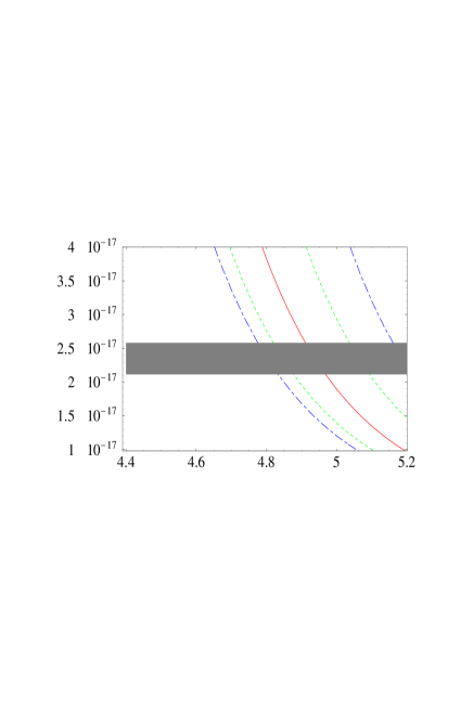
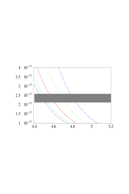
Figure 1: The 8th moment (in GeV^-16) as function of the bottom quark pole mass (in GeV) (upper figure) and the bottom quark PS mass (lower figure) at $\mu_{f}=2\,$GeV. The solid curve is for the scale $\hat{\mu}=2m_{b}/\sqrt{8}$, the outer (dash-dotted) curves show the result, when the scale is varied by a factor of 2 in both directions. The inner (dotted) curves correspond to $2\hat{\mu}/3$ and $3\hat{\mu}/2$. The experimental moment is given by the grey bar.

In Fig. 1, we show the result for the 8th moment as a function of the quark mass. In the upper figure, the result is plotted as a function of the pole mass $m_{b}$, in the lower figure as a function of the PS mass $m_{b,\rm PS}(2\,\mbox{GeV})$. For a given moment $n$, the integral (1) implies the characteristic energy scale $E\sim m_{b}/n$. The logarithms that appear in the PNRQCD integrals then suggest that the scale $\mu$ is chosen as $2m_{b}/\sqrt{n}$. This choice is shown as the solid line in the figure, together with variations by a factor $1/2,2/3,3/2,2$. In case of the pole mass as an input parameter, the scale dependence is very large. Including a (small in comparison) error due to the variation of $\alpha_{s}(M_{Z})=0.118\pm 0.003$, we determine $m_{b}=(4.97\pm 0.17)\,$GeV, where the scale error is estimated from a variation between $2\,$GeV and $2\hat{\mu}$. The scale dependence is somewhat reduced, but still large, with the PS mass as input. Our result is

$$m_{b,\rm PS}(2\,\mbox{GeV})=(4.60\pm 0.125(\mbox{scale})\pm 0.03(\alpha_{s})\pm 0.03(\mbox{exp.}))\,\mbox{GeV},$$ (14)

which translates into

$$\overline{m}_{b}(\overline{m}_{b})=(4.26\pm 0.12)\,\mbox{GeV}$$ (15)

for the $\overline{\rm MS}$ mass. We have included an estimate of $(40\pm 40)\,$MeV for the unknown 3- and 4-loop terms in the relation between the PS and the $\overline{\rm MS}$ mass, which are needed here, because the sum rule determines the PS mass with a parametric accuracy of order $m_{b}\alpha_{s}^{4}$. The central value is stable against variations of the order of the moments. The large remaining scale dependence can be traced to the scale dependence of the theoretical prediction of the first bound state residue. This is discussed in more detail in Ref. $\!{}^{{\bf?}}$.

$$\begin{array}[]{|c|c|c|c|}\hline\cr&m_{b}&\overline{m}_{b}(\overline{m}_{b})&\mbox{Remarks}\\ \hline\cr\mbox{This work}&4.97\pm 0.17&4.26\pm 0.12&\mbox{Sum rules}\\ \mbox{PP98 \immediate{$\!{}^{{\bf?}}$}}&4.80\pm 0.06&\mbox{--}&\mbox{Sum rules}\\ \mbox{H98 \immediate{$\!{}^{{\bf?}}$}}&4.88\pm 0.10&4.25\pm 0.09&\mbox{Sum rules}\\ \mbox{MY98 \immediate{$\!{}^{{\bf?}}$}}&\mbox{--}&4.20\pm 0.10&\mbox{Sum rules}\\ \hline\cr\mbox{JP97/98 \immediate{$\!{}^{{\bf?},{\bf?}}$}}&4.60\pm 0.02&4.19\pm 0.06&\mbox{Sum rules, no resummation}\\ \hline\cr\mbox{PY98 \immediate{$\!{}^{{\bf?}}$}}&5.00^{+0.10}_{-0.07}&4.44^{+0.03}_{-0.04}&\Upsilon(\mbox{1S})\mbox{ mass}\\ \mbox{MS98 \immediate{$\!{}^{{\bf?}}$}}&\mbox{--}&4.41\pm 0.11&\mbox{lattice HQET}\\ \hline\cr\end{array}$$

Table 1: Bottom quark mass values (in GeV) obtained from NNLO calculations.

In Tab. 1 we compare our result to other bottom quark mass results, choosing only NNLO calculations (although NNLO may not imply a NNLO resummation in some cases). The first four entries all refer to the sum rule method with NNLO resummation. There are several differences between the present and previous implementations of the NNLO moments. The summation of NLO logarithms of $v$, which has not been done in Refs. $\!{}^{{\bf?},{\bf?},{\bf?}}$, turns out to be a small effect; leaving it out would increase our result by up to $10\,$MeV. Refs. $\!{}^{{\bf?},{\bf?}}$ use the ‘old’ value of $a_{2}$ $\!{}^{{\bf?}}$, which is most likely incorrect $\!{}^{{\bf?}}$. Again, the corrected value for $a_{2}$ shifts the extracted quark mass downwards by only 15 MeV. More significant differences arise in the treatment of the short-distance factor and the bound state pole $\delta$-functions. For a detailed discussion we refer to Ref. $\!{}^{{\bf?}}$.

The sum rule calculation of Refs. $\!{}^{{\bf?},{\bf?}}$ does not include a non-relativistic resummation. It leaves out, in particular, the contribution from the Coulomb poles. This seems to be the main reason why the bottom masses of JP97/98 come out small. The large moments used in Refs. $\!{}^{{\bf?},{\bf?}}$ are completely dominated by the Coulomb pole contribution to (12). For the 8th moment, we find that our pole quark mass would decrease by roughly 400 MeV, if we left out the Coulomb pole contribution.

The last two entries in the table come from other methods. Ref. $\!{}^{{\bf?}}$ uses the NNLO result for the Coulomb pole position and compares it with the $\Upsilon(\mbox{1S})$ mass. The error quoted in Ref. $\!{}^{{\bf?}}$ is probably underestimated, because the scale $\mu^{2}$ is allowed to vary only by $\pm 25\%$ rather than a factor of 2. The origin of the large value of the $\overline{\rm MS}$ quark mass in Ref. $\!{}^{{\bf?}}$ will be explained in Ref. $\!{}^{{\bf?}}$. The last entry refers to the first complete NNLO quark mass determination from the lattice, based on the $B$ meson mass and the lattice measurement of the static energy of a heavy quark.

References

References

- [1] V.A. Novikov et al., Phys. Rev. Lett. 38, 626 (1977) [Erratum: ibid. 38, 791 (1977)]; Phys. Rep. 41, 1 (1978).
- [2] M.B. Voloshin and Yu.M. Zaitsev, Usp. Fiz. Nauk. 152, 361 (1987) [Sov. Phys. Usp. 30(7), 553 (1987)].
- [3] M.B. Voloshin, Int. J. Mod. Phys. A 10, 2865 (1995).
- [4] M. Beneke and V.A. Smirnov, Nucl. Phys. B 522, 321 (1998).
- [5] W.E. Caswell and G.P. Lepage, Phys. Lett. B 167, 437 (1986).
- [6] T. Kinoshita and M. Nio, Phys. Rev. D 53, 4909 (1996).
- [7] M. Beneke, A. Signer and V.A. Smirnov, Phys. Lett. B 454, 137 (1999).
- [8] M. Beneke and A. Signer, CERN-TH/99-163 [hep-ph/9906475].
- [9] M. Beneke, Talk given at 33rd Rencontres de Moriond: Electroweak Interactions and Unified Theories, Les Arcs, France, 14-21 Mar 1998 [hep-ph/9806429].
- [10] A.A. Penin and A.A. Pivovarov, Nucl. Phys. B 549, 217 (1999); Phys. Lett. B 435, 413 (1998).
- [11] A. Hoang, Phys. Rev. D 59, 014039 (1999).
- [12] K. Melnikov and A. Yelkhovsky, Phys. Rev. D 59, 114009 (1999).
- [13] A. Pineda and J. Soto, Nucl. Phys. Proc. Suppl. 64, 428 (1998) [hep-ph/9707481]; Phys. Lett. B 420, 391 (1998); Phys. Rev. D 59, 016005 (1999).
- [14] B.A. Thacker and G.P. Lepage, Phys. Rev. D 43, 196 (1991).
- [15] G.P. Lepage et al., Phys. Rev. D 46, 4052 (1992).
- [16] M. Beneke, A. Signer and V.A. Smirnov, Phys. Rev. Lett. 80, 2535 (1998).
- [17] A. Czarnecki and K. Melnikov, Phys. Rev. Lett. 80, 2531 (1998).
- [18] Y. Schröder, Phys. Lett. B 447, 321 (1999).
- [19] A.H. Hoang and T. Teubner, Phys. Rev. D 58, 114023 (1998).
- [20] M. Beneke and V.M. Braun, Nucl. Phys. B 426, 301 (1994); M. Beneke, Phys. Lett. B 344, 341 (1995).
- [21] I.I. Bigi, M.A. Shifman, N.G. Uraltsev and A.I. Vainshtein, Phys. Rev. D 50, 2234 (1994).
- [22] M. Beneke, Phys. Lett. B 434, 115 (1998).
- [23] A.H. Hoang, M.C. Smith, T. Stelzer and S. Willenbrock, Phys. Rev. D 59, 114014 (1999).
- [24] N. Gray, D.J. Broadhurst, W. Grafe and K. Schilcher, Z. Phys. C 48, 673 (1990).
- [25] K.G. Chetyrkin, J.H. Kühn and M. Steinhauser, Phys. Lett. B 371, 93 (1996); Nucl. Phys. B 482, 213 (1996); Nucl. Phys. B 505, 40 (1997).
- [26] M. Jamin and A. Pich, Nucl. Phys. B 507, 334 (1997).
- [27] M. Jamin and A. Pich, Nucl. Phys. Proc. 74, 300 (1999) [hep-ph/9810259].
- [28] A. Pineda and F.J. Yndurain, [hep-ph/9812371].
- [29] G. Martinelli and C.T. Sachrajda, [hep-lat/9812001].
- [30] M. Peter, Phys. Rev. Lett. 78, 602 (1997); Nucl. Phys. B 501, 471 (1997).