CERN-TH/99-163

DTP/99/60

hep-ph/9906475

The bottom $\overline{\rm MS}$ quark mass from sum rules
at next-to-next-to-leading order
M. Beneke Theory Division, CERN, CH-1211 Geneva 23, Switzerland
A. Signer Department of Physics, University of Durham,
Durham DH1 3LE, England

(June, 22, 1999)

We determine the bottom $\overline{\rm MS}$ quark mass $\overline{m}_{b}$ and the quark mass in the potential subtraction scheme from moments of the $b\bar{b}$ production cross section and from the mass of the Upsilon 1S state at next-to-next-to-leading order in a reorganized perturbative expansion that sums Coulomb exchange to all orders. We find $\overline{m}_{b}(\overline{m}_{b})=(4.25\pm 0.08)\,$GeV and $m_{b,\rm PS}(2\,\mbox{GeV})=(4.59\pm 0.08)\,$GeV for the potential-subtracted mass at the scale $2\,$GeV, adopting a conservative error estimate.

Introduction. Accurate determinations of the bottom quark mass in perturbative QCD usually rely on properties of the spectrum of Upsilon mesons and $b\bar{b}$ production near threshold. Since already for the $\Upsilon(\mbox{1S})$ state the momentum scale $p=m_{b}C_{F}\alpha_{s}(p)/2\sim 1.25\,$GeV and energy scale $E=m_{b}(C_{F}\alpha_{s}(p))^{2}/4\,\,\hbox to0.0pt{\lower 4.0pt\hbox{$\mathchar 0\relax\sim$}\hss}\raise 1.0pt\hbox{$<$}\,\,0.3\,$GeV are too small for perturbation theory to be expected to to work, one considers averages over the $b\bar{b}$ production cross section through a virtual photon, including the $\Upsilon$ resonances [1]:

$$M_{n}/(10\,\mbox{GeV})^{2n}\equiv\frac{12\pi^{2}}{n!}\,\frac{d^{n}}{d(q^{2})^{n}}\,\Pi(q^{2})_{\big{|}q^{2}=0}=\int\limits_{0}^{\infty}\!\frac{ds}{s^{n+1}}\,R_{b\bar{b}}(s).$$ (1)

In this case the characteristic momentum and energy scales are replaced by $p\sim 2m_{b}/\sqrt{n}$ and $E\sim m_{b}/n$, respectively. The requirement of perturbativity puts an upper limit on the admissible values of $n$. On the other hand, only the resonance contribution to the sum rule is experimentally well known, and $n$ needs to be taken large enough to reduce the error from the $b\bar{b}$ continuum. When $n\gg 1$, the perturbative expansion of $M_{n}$ in the strong coupling $\alpha_{s}$ breaks down, because there exist terms of the form $(\alpha_{s}\sqrt{n}\,)^{k}$ in any order of perturbation theory. This suggests a summation of the perturbative expansion to all orders in which $\alpha_{s}\sqrt{n}$ is treated as order 1 [2].

In this letter we analyse the sum rule (1) at next-to-next-to-leading order (NNLO) in this resummed perturbative expansion. [A preliminary analysis was presented in Ref. [3].] The resummed perturbative $b\bar{b}$ cross section is computed at NNLO using recent 2-loop results on the Coulomb potential [4] and the $\gamma^{*}b\bar{b}$ vertex [5, 6, 7] and non-relativistic effective field theory in dimensional regularization as described in [3, 8, 9]. Rather than determining the $b$ quark pole mass, as has usually been done, we apply the potential subtraction (PS) scheme and determine the PS mass [10] from the sum rule. We expect perturbative corrections in this and related schemes to be smaller than in the on-shell scheme [10, 11]. We then convert the extracted PS mass to the $\overline{\rm MS}$ mass, thus by-passing the infrared sensitivity problem of the on-shell scheme [12], and yet implementing the resummation necessary in the non-relativistic kinematics enforced by taking large moments. Other NNLO analyses of the sum rule have already appeared [13, 14, 15, 16]. Nevertheless, we think that an independent analysis, together with a critical discussion of the quark mass error, is still useful. We also perform a complementary analysis and determine the $b$ quark mass directly from the mass of the $\Upsilon(\mbox{1S})$ state. This has been done previously in a NNLO analysis presented in [17], which, however, concentrated on the $b$ quark pole mass, as did [13, 14].

Experimental moments. We first evaluate the integrals (1) by expressing the cross section in terms of the six $\Upsilon$ resonances and the open $b\bar{b}$ continuum. The masses and leptonic widths of the resonances are taken from [18]. Very little information exists on the $b\bar{b}$ continuum above $s=(10.56\,\mbox{GeV})^{2}$ [19]. We parametrize the continuum by setting $R_{b\bar{b}}^{cont.}=0.4\pm 0.2$. With this crude parametrization the experimental error on the determination of $m_{b}$ is $110\,(50,30,15)\,$MeV for $n=4\,(6,8,12)$, and small compared to the theoretical error for interesting moments with $n\sim 8$-$12$. Some experimental moments are shown in Table 1. For $n=8$-$12$ about 70%-85% of the experimental moment comes from the $\Upsilon(\mbox{1S})$ resonance.

$${\small\begin{array}[]{c|c|c|c|c|c}\hline\cr\hline\cr n&4&8&10&12&16\\ \hline\cr M_{n}&0.231\pm 0.044&0.235\pm 0.023&0.264\pm 0.021&0.308\pm 0.021&0.443\pm 0.025\\ \hline\cr\hline\cr\end{array}}\vspace*{-0.2cm}$$

Table 1: The experimental moments.

Theoretical moments. The theoretical moments are computed by first matching QCD to non-relativistic QCD. In a second step this theory is matched to a non-local Schrödinger field theory, in which $b\bar{b}$ pairs propagate through the Coulomb Green function. We then solve the Schrödinger equation to NNLO. We refer to [3, 8, 9] for some details of the method; further useful information can be found in [13, 14, 15]. The result for the $b\bar{b}$ cross section to NNLO, still in the on-shell scheme, is expressed as

$$R_{b\bar{b}}(s)=\alpha_{s}\left\{f_{0}(\lambda,l)+\alpha_{s}\,f_{1}(\lambda,l)+\alpha_{s}^{2}\,f_{2}(\lambda,l)\right\},$$ (2)

where $l=\ln(-4m_{b}E/\mu^{2})$, $\lambda=C_{F}\alpha_{s}/(2\,(-E/m_{b})^{1/2})$, $C_{F}=4/3$, $E=\sqrt{s}-2m_{b}$ and $m_{b}$ is the $b$ pole mass. The functions $f_{i}(\lambda,l)$ contain bound-state poles that correspond to the $\Upsilon(\mbox{nS})$ resonances. We obtained these functions analytically. After integrating numerically over $s$ according to (1), these functions sum all terms of the form $\alpha_{s}^{0,1,2}\,(\alpha_{s}\sqrt{n})^{k}$ to all orders. Writing $R_{b\bar{b}}(s)$ in the form of (2) implies that we expand the bound-state pole $\delta$-functions around the leading-order pole position. Expanding the bound-state pole $\delta$-functions rather than leaving them unexpanded is motivated by the fact that the sum rule relies on global duality. Using dispersion relations, the moments can be expressed in terms of derivatives of the vacuum polarization as indicated in (1), which makes no reference to individual resonances. Computing these derivatives in resummed perturbation theory to NNLO implies that we expand the resonance $\delta$-functions in the expression for $R_{b\bar{b}}(s)$.

Before integrating over $s$, we convert the expression for $R_{b\bar{b}}(s)$ from the on-shell to the potential subtraction scheme. The pole mass is eliminated using the relation [10]

$$m_{b} = m_{b,\rm PS}(\mu_{f})-\frac{1}{2}\int\limits_{|\vec{q}\,|<\mu_{f}}\!\!\!\frac{d^{3}\vec{q}}{(2\pi)^{3}}\,\tilde{V}(q)$$ (3)

$$= m_{b,\rm PS}(\mu_{f})+\frac{C_{F}\alpha_{s}}{\pi}\,\mu_{f}\left[1+\frac{\alpha_{s}}{4\pi}\,\delta m_{1}+\left(\frac{\alpha_{s}}{4\pi}\right)^{\!2}\,\delta m_{2}+\ldots\right],$$

where $\tilde{V}(q)$ is the Coulomb potential in momentum space. Explicit expressions for $\delta m_{1,2}$ can be found in [10]. Note that $m_{b}-m_{b,\rm PS}(\mu_{f})$ is proportional to a subtraction scale $\mu_{f}$, which should not exceed the characteristic scale $2m_{b}/\sqrt{n}$ of the moments $M_{n}$. We insert (3) into (2) and expand the small correction terms involving $\delta m_{1,2}$. However, the term $\Delta=C_{F}\alpha_{s}\mu_{f}/\pi$ is not expanded when $m_{b}$ is replaced in $E$, $\lambda$ or $l$, because $\Delta$ counts as being of the same order as $E=\sqrt{s}-2m_{b}$. The result is an expression of the same form as (2), but with $m_{b,\rm PS}(\mu_{f})$ as input parameter. As mentioned in the introduction we expect the expansion (2) in this new variable to be more convergent, and hence the PS mass can be determined with smaller error than the pole mass. The PS mass depends on $\mu_{f}$ and we choose $\mu_{f}=2\,$GeV as our default. The PS masses for different $\mu_{f}$ are connected by a renormalization group equation that follows directly from the definition (3).

The dominant theoretical uncertainty arises from the residual dependence of the theoretical moments on the renormalization scale $\mu$ of the strong coupling $\alpha_{s}\equiv\alpha_{s}(\mu)$ in the $\overline{\rm MS}$ scheme. We now discuss the choice and variation of this scale and the choice of moments $n$ that go into our analysis.

As indicated in (2) explicit logarithms of $\mu$ always come as $\ln(-4m_{b}E/\mu^{2})$. When $n\gg 1$, the integral (1) falls exponentially as $\exp(-nE/m_{b})$, so that the characteristic energy scale is $E\sim m_{b}/n$. This determines the parametric form of the renormalization scale to be $\mu_{n}\equiv 2m_{b}/\sqrt{n}$. This, however, is not strictly true, because the moments also contain parts in which gluons carry momentum of order $m_{b}$ and momentum of order $m_{b}/n$. In the renormalization-group-improved treatment (see [3, 9]) the hard scale $m_{b}$ enters as the starting point $\mu_{h}\sim m_{b}$ of the renormalization group evolution of the Wilson coefficient functions. The dependence on $\mu_{h}$ is negligible, of the order of $\pm 10\,$MeV on the output for $m_{b}$, compared to the dependence on the scale $\mu_{n}$, which determines the endpoint of the renormalization-group evolution. It is therefore not considered further. Gluons with three-momentum of order $m_{b}/n$ enter only at order $\alpha_{s}^{3}$. This leaves us with the scale $\mu_{n}$ above and we adopt $\mu_{n}\equiv 2m_{b}/\sqrt{n}$ as the most ‘natural’ scale.

One may object that the form of the logarithm gives the natural scale only parametrically, but that the scale is arbitrary up to a multiplicative factor, since the physical scale in the $\overline{\rm MS}$ scheme corresponds to a different scale in another scheme, for instance MS. We can address this question by searching for constants that appear systematically in conjunction with the logarithm $\ln(-4m_{b}E/\mu^{2})$. While this is complicated for the full cross section, it is easily done for the bound state energies that correspond to the $\Upsilon(\mbox{nS})$ resonances. We find that for the $k$th energy level the analogous logarithm always appears in the combination $\ln(m_{b}C_{F}\alpha_{s}/(k\mu))-S_{1}(k)$, where $S_{1}(k)\equiv\sum_{m=1}^{k}1/m$. Since $S_{1}(k)>0$, this suggests – if anything –, that the physical scale is even smaller than what we inferred from the logarithm alone.

The useful moments are restricted from below by the uncertainty in the experimental value of the moment. If we aim at an error of about $50\,$MeV in the determination of the $b$ quark mass, we need $n\geq 6$. There is also a technical restriction, which could be overcome. Our expression for $M_{n}$ sums all terms of the form $\alpha_{s}^{0,1,2}(\alpha_{s}\sqrt{n})^{k}$, but it does not make use of the exact fixed-order coefficients at order $\alpha_{s}^{1,2}$, which are known [20], because terms of relative order $n^{-3/2}$ or smaller are dropped. This could be compensated for by matching the resummed result and the fixed-order result. However, we find that for $n\geq 6$ this matching correction is small, as can be seen from Table 2.

It is advantageous to take large moments, because large moments are more sensitive to $m_{b}$, while the experimental error does not increase, see Table 1. An upper limit arises, because the characteristic scales must remain perturbative. As concerns $\mu_{n}$, the requirement $\mu_{n}>\Lambda_{\rm QCD}$ does not seem to pose a serious restriction. In practice, we find that the theoretical prediction becomes unstable already when $\mu$ is smaller than 1.5-2.0 GeV; requiring $\mu$ to be larger than this is restrictive, if we also allow for a variation of $\mu$ about $\mu_{n}$. A more serious constraint arises from the scale $m_{b}/n$, which enters the NNLO calculation implicitly. At NNNLO there is a contribution to the moment that scales as $\alpha_{s}(\mu_{n})^{2}\alpha_{s}(m_{b}/n)$. When $m_{b}/n\sim\Lambda_{\rm QCD}$, we should count $\alpha_{s}(m_{b}/n)$ as order 1. In this case, we have an uncontrolled non-perturbative contribution to the moments that is formally of NNLO. We therefore require $n\leq 10$. In the literature larger moments are often used. The justification for this is that the gluon condensate contribution to the moments, which represents the leading non-perturbative power correction, is small even for moments much larger than 10. However, the operator product expansion in local operators is itself only valid when $m_{b}/n>\Lambda_{\rm QCD}$ and so the estimate is not rigorous. It may, however, indicate that ultrasoft contributions from the scale $m_{b}/n$ are smaller than what we would estimate on parametric grounds.

For reference we give some selected moments in Table 2 in the on-shell and PS scheme. The table also quantifies the importance of resumming $(\alpha_{s}\sqrt{n})^{k}$ corrections and the error incurred by not including the exact fixed-order coefficients at order $\alpha_{s}^{1,2}$. Resummation is crucial even for $n=6$, because the contribution from the bound-state poles, which does not exist in the NNLO fixed-order approximation, is large. On the other hand, already for $n=6$ the fixed-order moments (FO1) are well approximated by the leading three terms in their large-$\sqrt{n}$ expansion (FO2).

$${\small\begin{array}[]{c||c|c|c||c|c|c||c|c|c}\hline\cr\hline\cr&\lx@intercol\hfil\mbox{LO}\hfil\lx@intercol\vrule\lx@intercol\vrule\lx@intercol&\lx@intercol\hfil\mbox{NLO}\hfil\lx@intercol\vrule\lx@intercol\vrule\lx@intercol&\lx@intercol\hfil\mbox{NNLO}\hfil\lx@intercol\\ \hline\cr n&\mbox{Res.}&\mbox{FO1}&\mbox{FO2}&\mbox{Res.}&\mbox{FO1}&\mbox{FO2}&\mbox{Res.}&\mbox{FO1}&\mbox{FO2}\\ \hline\cr 6&0.134\,[0.228]&0.030&0.028&0.127\,[0.143]&0.062&0.065&0.201\,[0.222]&0.094&0.097\\ \hline\cr 10&0.122\,[0.268]&0.016&0.016&0.143\,[0.166]&0.041&0.042&0.266\,[0.322]&0.073&0.075\\ \hline\cr 14&0.139\,[0.379]&0.011&0.011&0.190\,[0.218]&0.032&0.033&0.400\,[0.529]&0.065&0.067\\ \hline\cr\hline\cr\end{array}}\vspace*{-0.2cm}$$

Table 2: Selected moments (recall the normalization of the moments in (1)) in the on-shell and PS scheme (square brackets) for $\alpha_{s}(M_{Z})=0.118$ and $m_{b}=4.95\,$ GeV (on-shell scheme) and $m_{b,\rm PS}(2\,\mbox{GeV})=4.55\,$GeV (PS scheme). The renormalization scale is taken to be $\mu_{n}=2M/\sqrt{n}$, where $M=m_{b}$ or $M=m_{b,\rm PS}(2\,\mbox{GeV})$. ‘Res.’ refers to the resummed cross section with LO, NLO, NNLO in the sense of (2). ‘FO1’ refers to the fixed-order result without resummation, including terms of order $\alpha_{s}^{0,1,2}$ (LO, NLO, NNLO). ‘FO2’ refers to the fixed-order result, dropping terms with relative suppression $n^{-3/2}$ or more. The effect of resummation is given by the difference of ‘Res.’ and ‘FO2’. The correction due to matching to the fixed-order result is roughly given by ‘FO1’ minus ‘FO2’.

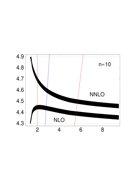
Figure 1: The value of $m_{b,\rm PS}(2\,\mbox{GeV})$ obtained from the 10th moment as a function of the renormalization scale in NLO and NNLO and for $\alpha_{s}(m_{Z})=0.118$. The dark region specifies the variation due to the experimental error on the moment. The middle line marks the scale $\mu_{n}$, the two outer lines determine the scale variation from which the theoretical error is computed.

Numerical analysis. For a given $n$ the theoretical moments are functions of $m_{b,\rm PS}(\mu_{f})$, which we would like to determine; the strong coupling $\alpha_{s}$, for which we use $\alpha_{s}(m_{Z})=0.118\pm 0.003$ together with 3-loop evolution; and the renormalization scale $\mu$, which is our (rough) handle to estimate the uncertainty due to the NNLO approximation of the moment calculation. We first compute, for given $n$ and $\mu$ (and $\alpha_{s}(m_{Z})=0.118$), the values of $m_{b,\rm PS}(2\,\mbox{GeV})$, for which the theoretical moment lies within the experimental range. For $n=10$ the result is shown in Fig. 1. It is evident that the resulting $m_{b,\rm PS}(2\,\mbox{GeV})$ varies significantly as function of the scale $\mu$ at which the sum rule is evaluated. Furthermore, there is no overlap between the range of masses that is obtained from the NNLO and the NLO sum rule for any reasonable range of $\mu$. The same conclusion is obtained for $n=6$ or $8$. We also determined $m_{b,\rm PS}(2\,\mbox{GeV})$ from $n=6,8,10$ simultaneously by minimizing a $\chi^{2}$ with equal weights. The value we obtain from this procedure differs by no more than $30\,$MeV from that obtained from single moments, when $\mu$ is varied between $1.5$ and $9.5\,$GeV, reflecting that the $\mu$-dependence of the theoretical moments is completely correlated. The same analysis in the on-shell scheme results in an identical qualitative picture; however, the scale-dependence is even larger in the on-shell scheme.

As explained above, we take $\mu_{n}=2m_{b,\rm PS}(\mu_{f})/\sqrt{n}$ as our default choice of scale. We would then follow common practice and estimate a theoretical error by varying the scale between one half and twice this value. But from Fig. 1 we observe that the theoretical prediction becomes unstable (compare the behaviour of the NLO and NNLO results) for scales below $2\,$GeV and one may argue that varying the scale into this region does not provide a reliable error estimate. We therefore compute the theoretical error from a variation between $2\,$GeV and $2\mu_{n}$. It is clear that the error so estimated is rather sensitive to the lower scale cut-off. Taking $n=10$ and adding the error from $\alpha_{s}$ and the experimental moments, we obtain

$$m_{b,\rm PS}(2\,\mbox{GeV})=(4.60\pm 0.10\,(\mbox{scale})\pm 0.03\,(\alpha_{s})\pm 0.02\,(\mbox{exp.}))\,\mbox{GeV}.$$ (4)

If the scale is varied down to $2.5\,(1.5)\,$GeV, the scale error decreases (increases) to $\pm\,65\,(160)\,$MeV. In comparison, a NLO analysis of the sum rule would return the central value $m_{b,\rm PS}(2\,\mbox{GeV})=4.44\,$GeV with a smaller scale uncertainty (see Fig. 1). The large difference with the NNLO result casts doubt on the convergence of successive perturbative approximations. The origin of this difference and the origin of the large scale dependence will become clear below.

The PS mass is a useful parameter (replacing the pole mass) for short-distance observables involving $b$ quarks close to their mass shell. For high energy processes, we would like to convert the PS mass to the $\overline{\rm MS}$ definition. Call $\overline{m}_{b}$ the $\overline{\rm MS}$ $b$ quark mass at the renormalization scale $\overline{m}_{b}$ and $k_{r}$ the coefficient at order $(\alpha_{s}(\overline{m}_{b})/(4\pi))^{r}$ that relates the pole mass to $\overline{m}_{b}$. From (3) we obtain the relation

$$m_{b,\rm PS}(\mu_{f})=\overline{m}_{b}\left(1+\sum_{r=1}^{\infty}\bigg{[}k_{r}-4C_{F}\delta m_{r-1}(\mu_{f})\,\frac{\mu_{f}}{\overline{m}_{b}}\,\bigg{]}\,\frac{\alpha_{s}(\overline{m}_{b})^{r}}{(4\pi)^{r}}\right),$$ (5)

where we defined $\delta m_{0}\equiv 1$. An N^kLO analysis of the sum rule determines the PS mass with a parametric accuracy of order $m_{b,\rm PS}\,\alpha_{s}^{k+2}$. This is most easily seen by noting that an N^kLO calculation of the resummed $b\bar{b}$ cross section determines the (perturbative) $\Upsilon(\mbox{nS})$ masses to order $m_{b,\rm PS}\alpha_{s}^{k+2}$. To determine the $\overline{\rm MS}$ mass with the same parametric accuracy implies that one should use (5) at order $\alpha_{s}^{k+2}$. At present (5) is known only to third order, combining the result of [21] for $k_{3}$ and the one for $\delta m_{2}(\mu_{f})$ from [10].

To obtain an order-of-magnitude estimate of the missing fourth-order term, we estimate the coefficient in the ‘large-$\beta_{0}$’ approximation [22, 23]. This gives $k_{4}=339071$ and $\delta m_{3}(2\,\mbox{GeV})=125026$ for $n_{f}=4$ and $\overline{m}_{b}=4.26\,$GeV. Although the individual coefficients are large, there are large cancellations in the combination that enters (5), which reflect the infrared cancellation that motivated the introduction of the potential subtraction [10]. With these numbers, given $m_{b,\rm PS}(2\,\mbox{GeV})$, we estimate that the $\alpha_{s}^{4}$ term reduces $\overline{m}_{b}$ by $10\,$MeV. (For comparison, the $\alpha_{s}^{3}$ term provides a $35\,$MeV reduction.) We therefore assume an additional $(10\pm 20)\,$MeV correction in the relation between $\overline{m}_{b}$ and $m_{b,\rm PS}(2\,\mbox{GeV})$ beyond the third-order formula. This results in the $\overline{\rm MS}$ mass

$$\overline{m}_{b}=(4.26\pm 0.09\,(\mbox{scale})\pm 0.01\,(\alpha_{s})\pm 0.02\,(\mbox{conv.})\pm 0.02\,(\mbox{exp.}))\,\mbox{GeV}.$$ (6)

The dependence on $\alpha_{s}$ nearly cancels out and ‘conv.’ refers to the conversion from the PS to the $\overline{\rm MS}$ scheme just discussed. We have repeated the analysis with $\mu_{f}=1\,$GeV and $3\,$GeV for the subtraction scale of the PS mass. Converting to $\overline{m}_{b}$, we find agreement with (6) within $20\,$MeV.

Origin of the large scale dependence. The scale uncertainty in (4) is only about 30% smaller than the uncertainty we would have found in the on-shell scheme. To understand the origin of this marginal improvement, we consider a truncated sum rule, in which both experimental and theoretical moments are given only in terms of the first $\Upsilon$ resonance. This is actually not a bad approximation to the full sum rule and allows us to discuss the origin of scale dependence in a transparent form. In this approximation, performing in addition a non-relativistic approximation to the $s$-integration measure in (1), we can write the sum rule as

$$\frac{\Gamma^{th}_{l^{+}l^{-}}}{\Gamma^{exp}_{l^{+}l^{-}}}=\exp\bigg{[}-(2n+1)\,\frac{M_{\Upsilon({\rm 1S})}^{exp}-M_{\Upsilon({\rm 1S})}^{th}}{M_{\Upsilon({\rm 1S})}^{exp}}\bigg{]},$$ (7)

where $\Gamma^{th}_{l^{+}l^{-}}$ and $M_{\Upsilon({\rm 1S})}^{th}$ are the leptonic width and mass of the $\Upsilon(\mbox{1S})$ state computed to NNLO. In the on-shell scheme, the series expansions for the two quantities read

$$M_{\Upsilon({\rm 1S})}^{th} = 2m_{b}-\frac{4}{9}\,m_{b}\alpha_{s}^{2}\,\bigg{(}1+\big{[}3.590-1.326\,l\big{]}\,\alpha_{s}+\big{[}19.52-6.033\,l+1.319\,l^{2}\big{]}\,\alpha_{s}^{2}\bigg{)},$$ (8)

$$= 2m_{b}-\frac{4}{9}\,m_{b}\alpha_{s}^{2}\,\bigg{(}1+1.08+1.76+\ldots\bigg{)}$$

$$\Gamma^{th}_{l^{+}l^{-}} = \frac{32}{27}\,e_{b}^{2}\alpha_{em}^{2}m_{b}\alpha_{s}^{3}\,\bigg{(}1+\big{[}3.605-1.989\,l-5.607\,\kappa\big{]}\,\alpha_{s}$$ (9)

$$+\,\big{[}24.14-7.898\,l+2.639\,l^{2}-0.3793\,\ln\kappa-20.21\kappa+11.16\,l\kappa+7.260\,\kappa^{2}\big{]}\,\alpha_{s}^{2}\bigg{)},$$

$$= \frac{32}{27}\,e_{b}^{2}\alpha_{em}^{2}m_{b}\alpha_{s}^{3}\,\bigg{(}1-0.11+1.23+\ldots\bigg{)}$$

where $\alpha_{s}=\alpha_{s}(\mu)$, $l=\ln(16m_{b}^{2}\alpha_{s}^{2}/(9\mu^{2}))$ and $\kappa=\alpha_{s}(m)/\alpha_{s}(\mu)$ and the second line is given for $\mu$ such that $l=0$ (for $m_{b}=5\,$GeV), in which case $\alpha_{s}(\mu)=0.30$. Neither of the series is converging and, because of the large power of $\alpha_{s}$ of the NNLO term, the scale dependence is huge at small scales, where $\alpha_{s}$ varies fast. This is seen from Fig. 2, which shows the scale dependence of the left-hand side and right-hand side of (7) separately.

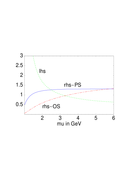
Figure 2: The left-hand side (lhs, short-dashed line) and right-hand side (rhs, dash-dotted and solid lines) of (7) as a function of the scale $\mu$ for $n=10$, $m_{b}=5\,$GeV (on-shell scheme, dash-dotted) and $m_{b,\rm PS}(2\,\mbox{GeV})=4.6\,$GeV (PS scheme, solid). The figure clearly shows the reduction of the scale dependence in the PS scheme for the predicted $\Upsilon({\rm 1S})$ mass. The scale dependence of the width (short-dashed line) is identical in the on-shell and PS schemes.

Going from the on-shell to the PS scheme improves the convergence and scale dependence of the predicted $\Upsilon({\rm 1S})$ mass as seen from the solid line in Fig. 2, but has little effect on the series expansion (9) for the width. Hence the large scale uncertainty in (4) can be traced to the poor control over the perturbative expansion for the leptonic width that controls the over-all normalization of the theoretical moments.

Constraints from $M_{\Upsilon({\rm 1S})}$. The fact that the mass determination from the sum rule is dependent on the theoretical prediction of the leptonic width, and limited in accuracy for this reason, suggests that we consider determining $m_{b}$ directly from the $\Upsilon$ spectrum. Non-perturbative corrections to the $\Upsilon$ masses grow rapidly for higher radial excitations and preclude using any state other than the ground state. The problem with this method is that even for the $\Upsilon(\mbox{1S})$ state it is difficult to estimate the non-perturbative correction reliably. The perturbative expression for the $\Upsilon(\mbox{1S})$ mass in the on-shell scheme is given by (8) above.

If $m_{b}(C_{F}\alpha_{s})^{2}/4\gg\Lambda_{\rm QCD}$, the non-perturbative correction to the $\Upsilon(\mbox{1S})$ mass can be computed in terms of vacuum condensates of local operators. The leading contribution is [24]

$$\delta M_{\Upsilon({\rm 1S})}^{\rm np}=\frac{624}{425}\,\pi m_{b}\,\frac{\langle\alpha_{s}GG\rangle}{(m_{b}C_{F}\alpha_{s})^{4}},$$ (10)

where $\langle\alpha_{s}GG\rangle\approx 0.05\,\mbox{GeV}^{4}$ is the gluon condensate. The actual magnitude of $\delta M_{\Upsilon({\rm 1S})}^{\rm np}$ is rather uncertain. If we choose the ‘natural’ scale $\mu=m_{b}C_{F}\alpha_{s}(\mu)\approx 2\,$GeV, we obtain $\delta M_{\Upsilon({\rm 1S})}^{\rm np}\approx 90\,$MeV. However, as noted earlier, the logarithm that determines this scale appears together with constants that tend to make the effective scale lower. Furthermore, it may be argued that the coupling $\alpha_{s}$ should be taken as the coefficient of $C_{F}/r$ in the Coulomb potential rather than in the $\overline{\rm MS}$ scheme. This coupling is larger than the $\overline{\rm MS}$ coupling. Both effects can decrease $\delta M_{\Upsilon({\rm 1S})}^{\rm np}$ substantially.

Since the inequality $m_{b}(C_{F}\alpha_{s})^{2}/4\gg\Lambda_{\rm QCD}$ that justifies the operator product expansion (OPE) does not hold, we should consider the subsequent term in the OPE to judge whether the expansion converges. Using the result of [25], we find that the contribution from dimension-6 operators could be anything between a fraction of and twice $-\delta M_{\Upsilon({\rm 1S})}^{\rm np}$, where the large uncertainty stems from the poorly known dimension-6 condensates and the ambiguity in the value of $\alpha_{s}$. This puts the convergence of the OPE in question. We therefore consider (10) as an order-of-magnitude estimate of the non-perturbative correction and treat it as a theoretical error rather than adding it to (8). In our opinion, assigning an error of $\pm 70\,$MeV to $m_{b}$ from this source is conservative.

We proceed to determine $m_{b,\rm PS}(\mu_{f})$ from $M_{\Upsilon({\rm 1S})}$ using (8) converted to the PS scheme. This renders the series (8) convergent and leads to a very small scale uncertainty of the extracted value of $m_{b,\rm PS}(2\,\mbox{GeV})$, as anticipated from the solid curve in Fig. 2. Varying $\mu$ from $1.25\,$ to $4\,$GeV, we obtain

$$m_{b,\rm PS}(2\,\mbox{GeV})=(4.58\pm 0.04\,(\mbox{scale})\pm 0.01\,(\alpha_{s})\pm 0.07\,(\mbox{non-pert.}))\,\mbox{GeV},$$ (11)

which is consistent with (4). In this case a NLO analysis would return the central value $m_{b,\rm PS}(2\,\mbox{GeV})=4.53\,$GeV, which suggests that the corresponding small value in the sum rule analysis is an anomaly related to the behaviour of the series for the leptonic width. From (11) we obtain the $\overline{\rm MS}$ mass

$$\overline{m}_{b}=(4.24\pm 0.04\,(\mbox{scale},\mu_{f})\pm 0.02\,(\alpha_{s})\pm 0.02\,(\mbox{conv.})\pm 0.07\,(\mbox{non-pert.}))\,\mbox{GeV}.$$ (12)

The central value varies by only about $10\,$MeV, when $\mu_{f}$ is varied between $1$ and $3\,$GeV. Contrary to the sum rule determination, the error is dominated by the non-perturbative contribution to the $\Upsilon(\mbox{1S})$ mass. This leaves room for improving upon the error, if some quantitative insight into the non-perturbative contribution could be obtained.

Comparison with previous results. We compare the bottom quark mass obtained in this work with the results of earlier NNLO analyses of the sum rule and the $\Upsilon(\mbox{1S})$ mass. Our comments will be restricted to those analyses that quote a result for the $\overline{\rm MS}$ quark mass [13, 14, 15, 16, 17, 26]. With the exception of [17], which obtains $\overline{m}_{b}$ from $M_{\Upsilon({\rm 1S})}$ and, therefore, should be compared with (12), all other NNLO analyses use the sum rule (1) and should be compared with (6).

The value given in (12) is significantly smaller than $\overline{m}_{b}=(4.44\pm 0.04)\,$GeV, obtained by [17]. This difference is explained by the fact that [17] first uses the on-shell scheme to extract the pole mass and then uses the 2-loop truncation of (5) [with $\mu_{f}=0$] to obtain $\overline{m}_{b}$. However, contrary to the PS scheme with $\mu_{f}=2\,$GeV, the 3-loop and 4-loop terms are large in the on-shell scheme; at least the 3-loop term has to be included when the pole mass is determined from the NNLO formula for the $\Upsilon(\mbox{1S})$ mass. Estimating the terms missing in [17] in the large-$\beta_{0}$ limit, and subtracting them from $\overline{m}_{b}=(4.44\pm 0.04)\,$GeV, we find that the result of [17] becomes (roughly) consistent with ours. The error estimate of [17] is, however, less conservative than ours.

A related difficulty concerns the comparison with the value $\overline{m}_{b}=(4.21\pm 0.11)\,$GeV quoted in [13]. While apparently consistent with the one obtained in this work, it is obtained via a 2-loop relation from the $b$ quark pole mass, which in turn is determined from the sum rule. If we add the 3-loop and/or 4-loop term, the result of [13] would be about $200\,$MeV lower than ours. This difference is a reflection of the fact that the pole mass quoted in [13] is roughly $200\,$MeV lower than the one we would have obtained had we chosen to determine it. This difference in turn can be traced to the use of a high renormalization scale for the evaluation of the sum rule, cf. Fig. 1. In our opinion, the choice of such a high scale is not well motivated. We also think that it is mandatory to use intermediate mass definitions such as the PS mass to determine $\overline{m}_{b}$ reliably. Otherwise large perturbative coefficients make it impossible to disentangle true theoretical errors from correlated and spurious ones caused by those large perturbative coefficients.

The most recent analysis by the authors of [26] determines the $\overline{\rm MS}$ mass directly from the sum rule and gives $\overline{m}_{b}=4.19\pm 0.06\,$GeV from moments with $n=7$-$15$. No resummation is performed, because it is assumed, incorrectly, that this is unnecessary in the $\overline{\rm MS}$ scheme. However, for high moments the Coulomb interaction must be treated non-perturbatively, and a resummation has to be done, irrespective of the mass renormalization convention. The $\overline{\rm MS}$ scheme actually makes the expansion worse, because the expansion contains terms of order $(\alpha_{s}n)^{k}$ in addition to $(\alpha_{s}\sqrt{n})^{k}$. To avoid such terms, one has to use an intermediate convention, such as the potential subtraction scheme, and then relate this convention to the $\overline{\rm MS}$ scheme in a second step. Because of this theoretical shortcoming, the result of [26] cannot be compared with (6).

The other papers quoted above perform a NNLO resummation as in this work. Differences arise either in the representation of the NNLO-resummed moments or in the analysis and error evaluation strategy. Both [15] (MY) and [16] (Hoang) also use intermediate mass subtractions, different from the PS scheme, but conceptually similar to it, before converting these intermediate masses to the $\overline{\rm MS}$ scheme.

The differences in the theoretical representation of the moments are the following:

• MY and Hoang use a factorization scheme different from dimensional regularization. Since the final result is physical, this is a technical difference that should bear no consequences on the final result.

• Hoang applies the non-relativistic approximation also to the $s$-integration in (1), while MY and the present work obtain the resummed cross section analytically and then integrate it numerically according to (1) or after an equivalent contour deformation into the complex $s$-plane. The difference is negligible.

• MY and Hoang have taken the short-distance coefficient as an over-all factor, while we have multiplied it out to NNLO. Keeping it as an over-all factor is problematic, because this results in a spurious factorization scheme and scale dependence, which is not small as can be seen from Table 3 of [16]. Since both short-distance and long-distance contributions are computed perturbatively, the factorization scale is a purely technical construct and no dependence on it should be left in the result. One motivation for writing the short-distance coefficient as an over-all factor is that the scales in the coupling constant are different in the long- and short-distance parts. However, this effect, related to logarithms of $n$, can be treated consistently only in the context of a full renormalization group treatment. This has been done in the present work (see [3, 9]), but not in [15, 16]. As a consequence there is no analogue of $\mu_{\rm fac}$ in the present approach, while the role of $\mu_{\rm hard}$ in [15, 16] is taken by the starting scale for the renormalization group evolution. As mentioned earlier, this dependence is negligible in our representation of the moments.

• Hoang and this work expand the bound-state $\delta$-functions for reasons discussed earlier; MY keep them unexpanded. This increases the theoretical moments significantly at NNLO. Not expanding the bound state $\delta$-functions would increase the value quoted in (4) and (6) by almost $100\,$MeV.

• MY and Hoang use a 2-loop formula to obtain $\overline{m}_{b}$ from their intermediate mass. As explained above, a NNLO analysis of the sum rule determines the PS (or related) masses with $m_{b}\alpha_{s}^{4}$ accuracy and to fully exploit this accuracy, the 4-loop relation between the PS and $\overline{\rm MS}$ mass should be used. We estimated that the 3- and 4-loop terms decrease $\overline{m}_{b}$ by $45\,$MeV and this additional shift has been incorporated in (6). Employing a less accurate relation entails a corresponding loss in parametric accuracy of $\overline{m}_{b}$, although this is a numerically small effect, if our estimate is correct.

As in this work, MY obtain their result from an analysis of single moments (checking consistency between a set of moments), although larger moments $n=14$-$18$ are used, which could be considered problematic. They use the so-called kinetic mass as intermediate mass definition. The analogue of $\delta m_{2}(\mu_{f})$ in (3), needed for a NNLO sum rule analysis, is not yet known in this scheme; MY estimate it in the large-$\beta_{0}$ limit, an additional assumption we had to use only for the 4-loop term when relating (4) to (6), but not to extract the PS mass in the first place. MY vary the renormalization scale from $2\,$GeV to $4.5\,$GeV, while we would argue that, for the high moments used in [15], the scale should be chosen lower. If we repeat our analysis with the same assumptions as those of MY, we reproduce their error estimate for the kinetic mass, which is smaller than the more conservative procedure that leads to (4).

Hoang uses an analysis and error estimate that is different from the single-moment analysis performed by MY and in this work. Simplifying somewhat, Hoang fits the quark mass from the linear combination $0.12M_{4}-0.56M_{6}+0.76M_{8}-0.31M_{10}$ of moments, where the coefficients are determined by the covariance matrix of the experimental input data such as the measured leptonic widths of the six $\Upsilon$ resonances. This linear combination (which entails a cancellation of one part in 4000) turns out to be very insensitive to the renormalization scale $\mu$, yet retaining a large sensitivity to $m_{b}$. Hoang then scans the theoretical parameter space and finds an error of only $\pm 30\,$MeV for the so-called 1S-mass, compared to the error of (4). We have repeated our analysis for this linear combination and obtain $m_{b,\rm PS}(2\,\mbox{GeV})=4.58\pm 0.02\,$GeV in this way, where the quoted error is due to variation of the renormalization scale only. The result is consistent with (4), but the error is much smaller. The central value is $50\,$MeV higher than the value reported in Sect. 6 of [16]. Such differences can be explained by different implementations of the NNLO result, as discussed above.

Several circumstances make us suspicious that the theoretical error is underestimated by Hoang’s procedure. For example, if we increase the error of the leptonic width of the $\Upsilon(\mbox{2S})$ by a factor of 10, or if we increase the error on the measured mass of the $\Upsilon(\mbox{1S})$ to $5\,$MeV, which is still small compared to the expected theoretical error, the procedure chooses a linear combination that exhibits less stability in $\mu$, and has no or two solutions for $m_{b,\rm PS}(2\,\mbox{GeV})$ for some ranges of $\mu$, even though our experimental knowledge of the width or mass should have no bearing on the theoretical error estimate. This remark may not be considered as a serious objection, because we could abandon the way the linear combination is chosen in [16] and optimize it deliberately. However, even for the original linear combination, there is a second solution $m_{b,\rm PS}(2\,\mbox{GeV})=4.86\pm 0.04\,$GeV in addition to $m_{b,\rm PS}(2\,\mbox{GeV})=4.58\pm 0.02\,$GeV, because the linear combination is no longer a monotonic function of $m_{b}$. The criterium of renormalization scale stability does not exclude obtaining solutions that differ by more than the error estimated from the $\mu$-dependence. The problem is compounded by the observation that the stability under variations of the renormalization scale, and hence the small error obtained by Hoang, crucially depends on the assumption that the four moments are combined at the same value of the renormalization scale $\mu$. This is a serious assumption, in particular as the natural scale of the moments is $2m_{b}/\sqrt{n}$. If we combine the moments at their natural rather than at equal scales, the stability is lost. To be fair, we should mention that Hoang’s analysis is more involved than analysing a single linear combination, although the covariance matrix is such that it does indeed give most weight to a single one. Nevertheless, we think that the simplified discussion above emphasizes the problem with estimating a theoretical error in the way done in [16].

The final results by MY ($\overline{m}_{b}=4.2\pm 0.1\,$GeV) and by Hoang ($\overline{m}_{b}=4.20\pm 0.06\,$GeV) agree with (6) within the quoted errors. However, if the $45\,$MeV shift were applied to those results, there is actually a discrepancy of about $100\,$MeV in the central value. This could be a consequence of the different representations of the moments as discussed above. However, we find it difficult to reconcile a $\overline{m}_{b}$ significantly smaller than $4.25\,$GeV with the analysis of $M_{\Upsilon({\rm 1S})}$ [see (12)], unless there is indeed a large positive non-perturbative contribution to $M_{\Upsilon({\rm 1S})}$.

Summary. We determined the bottom quark mass in the $\overline{\rm MS}$ scheme and the potential subtraction (PS) scheme [10] at next-to-next-to-leading order from sum rules for the $b\bar{b}$ cross section and the mass of the $\Upsilon(\mbox{1S})$ state. The results are in excellent agreement with each other as summarized by (4), (6), (11) and (12). There is no systematic procedure to combine the two results. On the one hand, the two determinations are not independent, because some theoretical input is common to both. On the other hand, the dominant source of theoretical error is different. We therefore combine the two determinations to yield the PS mass

$$m_{b,\rm PS}(2\,\mbox{GeV})=4.59\pm 0.08\,\mbox{GeV}$$ (13)

and the $\overline{\rm MS}$ mass (at the scale of the $\overline{\rm MS}$ mass)

$$\overline{m}_{b}(\overline{m}_{b})=4.25\pm 0.08\,\mbox{GeV}.$$ (14)

The calculations that go into these results imply partial resummations of the QCD perturbative expansion to all orders. An important point is that a NNLO resummation allows us to determine the quark masses with a parametric accuracy of order $m_{b}\alpha_{s}^{4}$, i.e. the residual error scales formally as $\delta m_{b}/m_{b}\sim\alpha_{s}^{5}$. In the case of the $\overline{\rm MS}$ mass this requires that one controls the four-loop relation to the PS mass. We estimated the 4-loop term, which is not yet known exactly and found that it should be very small.

Unfortunately, the sum rule analysis yields a much less precise determination of the bottom quark mass than what might have been expected with NNLO accuracy. We identify as the reason for this the bad behaviour of the perturbative expansion for the leptonic width of the $\Upsilon$ resonances. The same is true for the $\Upsilon(\mbox{1S})$ mass in the on-shell scheme. However, in this case it is understood that the large coefficients are unphysical and can be removed by a suitable mass subtraction procedure. If a similar mechanism underlied the expansion for the leptonic width, the error on the bottom quark mass could be reduced. In the absence of any understanding of this point, we have adopted a more conservative error estimate than in previous works [13, 14, 15, 16], mainly because of a more generous variation of the renormalization scale. Eq. (14) is in agreement within errors, but larger than the quark mass values quoted there, but is about $200\,$MeV smaller than the one in [17]. We argued that the result of [17] should be corrected for the large 3-loop term in the relation between the pole mass and the $\overline{\rm MS}$ mass.

Eq. (14) is also in good agreement with $\overline{m}_{b}(\overline{m}_{b})=4.26\pm 0.07\,\mbox{GeV}$ found in [28]. This work uses the $B$ meson mass, a lattice calculation of the (properly defined) binding energy of the $B$ meson in the unquenched, two-flavour approximation to heavy quark effective theory, and a two-loop perturbative matching to the $\overline{\rm MS}$ scheme. To our knowledge, this is the only other NNLO determination of the $\overline{\rm MS}$ mass besides the sum rule calculations mentioned above (which, in fact, are N⁴LO as far as $\overline{m}_{b}$ is concerned). However, because of the heavy quark limit, there are $1/m_{b}$ corrections, which remain to be estimated. Finally, the result is also in agreement with earlier, parametrically less accurate determinations, as for example in [29].

Acknowledgements. We thank G. Buchalla, A.H. Hoang and A. Pineda for useful discussions and comments on the manuscript. We also thank M. Steinhauser for providing us with the numerical code that produced the fixed-order moments (FO1) in Table 2. This work was supported in part by the EU Fourth Framework Programme ‘Training and Mobility of Researchers’, Network ‘Quantum Chromodynamics and the Deep Structure of Elementary Particles’, contract FMRX-CT98-0194 (DG 12 - MIHT).

References

- [1] V.A. Novikov et al., Phys. Rev. Lett. 38 (1977) 626 [Erratum: ibid. 38 (1977) 791]; Phys. Rep. 41 (1978) 1.
-
[2]
M.B. Voloshin and Yu.M. Zaitsev, Usp. Fiz. Nauk. 152 (1987) 361
[Sov. Phys. Usp. 30(7) (1987) 553];
M.B. Voloshin, Int. J. Mod. Phys. A10 (1995) 2865. - [3] M. Beneke, A. Signer and V.A. Smirnov, in: Proceedings of RADCOR98, Barcelona, September 1998. Note that the numerical result of the version published in the proceedings is affected by a program error, which is corrected in the hep-ph archive version [hep-ph/9906476].
-
[4]
Y. Schröder, Phys. Lett. 447 (1999) 321;
M. Peter, Phys. Rev. Lett. 78 (1997) 602. -
[5]
M. Beneke and V.A. Smirnov, Nucl. Phys. B522 (1998) 321;
M. Beneke, A. Signer and V.A. Smirnov, Phys. Rev. Lett. 80 (1998) 2535. - [6] A. Czarnecki and K. Melnikov, Phys. Rev. Lett. 80 (1998) 2531.
- [7] A. Hoang, Phys. Rev. D56 (1997) 7276.
- [8] M. Beneke, Talk given at 33rd Rencontres de Moriond: Electroweak Interactions and Unified Theories, Les Arcs, France, 14-21 Mar 1998 [hep-ph/9806429].
- [9] M. Beneke, A. Signer and V.A. Smirnov, Phys. Lett. B454 (1999) 137.
- [10] M. Beneke, Phys. Lett. B434 (1998) 115.
- [11] A.H. Hoang, M.C. Smith, T. Stelzer and S. Willenbrock, Phys. Rev. D59 (1999) 114014.
-
[12]
M. Beneke and V.M. Braun, Nucl. Phys. B426 (1994) 301;
M. Beneke, Phys. Lett. B344 (1995) 341;
I.I. Bigi, M.A. Shifman, N.G. Uraltsev and A.I. Vainshtein, Phys. Rev. D50 (1994) 2234. - [13] A.A. Penin and A.A. Pivovarov, Phys. Lett. B435 (1998) 413.
- [14] A.H. Hoang, Phys. Rev. D59 (1999) 014039.
- [15] K. Melnikov and A. Yelkhovsky, Phys. Rev. D59 (1999) 114009.
- [16] A.H. Hoang, [hep-ph/9905550].
- [17] A. Pineda and F.J. Yndurain, Phys. Rev. D58 (1998) 094022; [hep-ph/9812371].
- [18] Particle Data Group, C. Caso et al., Eur. Phys. J. C3 (1998) 1.
- [19] D.S. Akerib et al. [CLEO-II Collaboration], Phys. Rev. Lett. 67 (1991) 1692.
- [20] K.G. Chetyrkin, J.H. Kühn and M. Steinhauser, Phys. Lett. B371 (1996) 93; Nucl. Phys. B482 (1996) 213; Nucl. Phys. B505 (1997) 40.
- [21] K.G. Chetyrkin and M. Steinhauser, [hep-ph/9907509].
-
[22]
M. Beneke and V.M. Braun, Phys. Lett. 348 (1995) 513;
P. Ball, M. Beneke and V.M. Braun, Nucl. Phys. B452 (1995) 563. -
[23]
M. Neubert,
Phys. Rev. D51 (1995) 5924;
C.N. Lovett-Turner and C.J. Maxwell, Nucl. Phys. B452 (1995) 188. -
[24]
H. Leutwyler, Phys. Lett. B98 (1981) 447;
M.B. Voloshin, Sov. J. Nucl. Phys. 36(1) (1982) 143. - [25] A. Pineda, Nucl. Phys. B494 (1997) 213.
- [26] M. Jamin and A. Pich, Nucl. Phys. Proc. Suppl. 74 (1999) 300 [hep-ph/9810259]; Nucl. Phys. B507 (1997) 334.
- [27] A.H. Hoang, Z. Ligeti and A.V. Manohar, Phys. Rev. D59 (1999) 074017.
- [28] V. Giménez, L. Giusti, F. Rapuano and G. Martinelli, [hep-lat/9909138].
- [29] L.J. Reinders, H. Rubinstein and S. Yazaki, Phys. Rept. 127 (1985) 1; S. Narison, Phys. Lett. B341 (1994) 73.