Theoretical Constraints on the
Vacuum Oscillation Solution to the
Solar Neutrino Problem

The vacuum oscillation (VO) solution to the solar anomaly requires an extremely small neutrino mass splitting, $\Delta m^{2}_{sol}\stackrel{{\scriptstyle<}}{{{}_{\sim}}}10^{-10}\ {\rm eV}^{2}$. We study under which circumstances this small splitting (whatever its origin) is or is not spoiled by radiative corrections. The results depend dramatically on the type of neutrino spectrum. If $m_{1}^{2}\sim m_{2}^{2}\stackrel{{\scriptstyle>}}{{{}_{\sim}}}m_{3}^{2}$, radiative corrections always induce too large mass splittings. Moreover, if $m_{1}$ and $m_{2}$ have equal signs, the solar mixing angle is driven by the renormalization group evolution to very small values, incompatible with the VO scenario (however, the results could be consistent with the small-angle MSW scenario). If $m_{1}$ and $m_{2}$ have opposite signs, the results are analogous, except for some small (though interesting) windows in which the VO solution may be natural with moderate fine-tuning. Finally, for a hierarchical spectrum of neutrinos, $m_{1}^{2}\ll m_{2}^{2}\ll m_{3}^{2}$, radiative corrections are not dangerous, and therefore this scenario is the only plausible one for the VO solution.

CERN-TH/99-171

June 1999

IEM-FT-195/99

CERN-TH/99-171

IFT-UAM/CSIC-99-23

hep-ph/9906281

1 Introduction

There are three main explanations of the solar neutrino flux deficits, requiring oscillations of electron neutrinos into other species. Namely, the small and large angle MSW solutions, and the vacuum oscillation (VO) solution. In this paper we focus on the latter, which requires the relevant mass splitting and mixing angle in the range [1]

$$5\times 10^{-11}\ {\rm eV}^{2}< \Delta m^{2}_{sol} <1.1\times 10^{-10}\ {\rm eV}^{2},$$

$$\sin^{2}2\theta_{sol} > 0.67\,.$$ (1)

On the other hand, Superkamiokande observations [2] of atmospheric neutrinos require neutrino oscillations (more precisely $\nu_{\mu}-\nu_{\tau}$ oscillations if we do not consider oscillations into sterile species) driven by a mass splitting and a mixing angle in the range [1]

$$5\times 10^{-4}\ {\rm eV}^{2}< \Delta m^{2}_{atm} <10^{-2}\ {\rm eV}^{2}\ ,$$

$$\sin^{2}2\theta_{atm} > 0.82\ .$$ (2)

Let us remark the enormous hierarchy of mass splittings between the different species of neutrinos, $\Delta m^{2}_{sol}\ll\Delta m^{2}_{atm}$, which is apparent from eqs.(1, 2).

It has been argued that the extreme tinyness of $\Delta m^{2}_{sol}$ in this scenario could be related to some continuous or discrete symmetry at high energy [4]. However, independently of the origin of the small splittings, it must be required that their size is not spoiled by radiative corrections, the dominant part of which can be accounted by integrating the renormalization group equations (RGEs) between the scale at which the effective mass matrix is generated and low energy. The aim of this paper is to analyze under which circumstances this is in fact the case. As a result, we obtain important theoretical restrictions on the VO scenario.

Let us introduce now some notation. We define the effective mass term for the three light (left-handed) neutrinos in the flavour basis, $\nu^{T}=(\nu_{e},\nu_{\mu},\nu_{\tau})$, as

$${\cal L}=-\frac{1}{2}\nu^{T}{\cal M_{\nu}}\nu\;+\;{\rm h.c.}$$ (3)

The mass matrix, ${\cal M_{\nu}}$, is diagonalized in the usual way, i.e. ${\cal M_{\nu}}=V^{*}D\,V^{\dagger}$, where $D={\rm diag}(m_{1}e^{i\phi},m_{2}e^{i\phi^{\prime}},m_{3})$ and $V$ is a unitary ‘CKM’ matrix, relating flavour to mass eigenstates

$$\pmatrix{\nu_{e}\cr\nu_{\mu}\cr\nu_{\tau}\cr}=\pmatrix{c_{2}c_{3}&c_{2}s_{3}&s_{2}e^{-i\delta}\cr-c_{1}s_{3}-s_{1}s_{2}c_{3}e^{i\delta}&c_{1}c_{3}-s_{1}s_{2}s_{3}e^{i\delta}&s_{1}c_{2}\cr s_{1}s_{3}-c_{1}s_{2}c_{3}e^{i\delta}&-s_{1}c_{3}-c_{1}s_{2}s_{3}e^{i\delta}&c_{1}c_{2}\cr}\,\pmatrix{\nu_{1}\cr\nu_{2}\cr\nu_{3}\cr}\,.$$ (4)

Here, $s_{i}$ and $c_{i}$ denote $\sin\theta_{i}$ and $\cos\theta_{i}$, respectively, and in the rest of the paper we will neglect CP-violating phases. In the following, we label the mass eigenstates $\nu_{i}$ in such a way that $|\Delta m^{2}_{12}|<|\Delta m^{2}_{23}|\sim|\Delta m^{2}_{13}|$, where $\Delta m^{2}_{ij}\equiv m^{2}_{j}-m^{2}_{i}$ ($m_{\nu_{3}}^{2}$ is thus the most split eigenvalue). Consequently, $\Delta m^{2}_{sol}$, $\theta_{sol}$ correspond to $\Delta m^{2}_{12}$, $\theta_{3}$, while $\Delta m^{2}_{atm}$, $\theta_{atm}$ correspond to $\Delta m^{2}_{23}\sim\Delta m^{2}_{13}$, $\theta_{1}$ respectively. In our notation $\Delta m^{2}_{sol}$, $\Delta m^{2}_{atm}$ denote always the “experimental” splittings of eqs.(1, 2), while $\Delta m^{2}_{12}$, $\Delta m^{2}_{23}$ denote the computed splittings once the radiative corrections are incorporated. Concerning the $\theta_{2}$ angle, according to the most recent combined analysis of SK $+$ CHOOZ data (last paper of ref. [1]) it is constrained to have low values, $\sin^{2}2\theta_{2}<0.36\,(0.64)$ at 90% (99%) C.L.

We assume along the paper that the effective mass matrix for the left-handed neutrinos, ${\cal M}_{\nu}$, is generated at some high energy scale, $\Lambda$, by some unspecified mechanism. Below $\Lambda$, we consider two possibilities: either the effective theory is the Standard Model (SM) or the minimal supersymmetric Standard Model (MSSM) with unbroken $R-$parity. In the first case, the lowest dimension operator producing a mass term of this kind is uniquely given by [5]

$$-\frac{1}{4}\kappa\nu^{T}\nu HH\;+\;{\rm h.c.}$$ (5)

where $\kappa$ is a matricial coupling and $H$ is the ordinary (neutral) Higgs. Obviously, ${\cal M}_{\nu}=\frac{1}{2}\kappa\langle H\rangle^{2}$. The effective coupling $\kappa$ runs with the scale from $\Lambda$ to $M_{Z}$, with a RGE given by [6]

$$16\pi^{2}\frac{d\kappa}{dt}=\left[-3g_{2}^{2}+2\lambda+6Y_{t}^{2}+2{\rm Tr}{\bf Y_{e}^{\dagger}Y_{e}}\right]\kappa-\frac{1}{2}\left[\kappa{\bf Y_{e}^{\dagger}Y_{e}}+({\bf Y_{e}^{\dagger}Y_{e}})^{T}\kappa\right]\ ,$$ (6)

where $t=\log\mu$, and $g_{2},\lambda,Y_{t},{\bf Y_{e}}$ are the $SU(2)$ gauge coupling, the quartic Higgs coupling, the top Yukawa coupling and the matrix of Yukawa couplings for the charged leptons, respectively. The last term of eq.(6) is the most important one for our purposes, since it modifies the texture of ${\cal M}_{\nu}$. It is worth noticing that the modification of a mass eigenvalue is always proportional to the mass eigenvalue itself. In the MSSM case, things are very similar but with an important difference. Namely, the term that modifies the texture in the RGEs has the same form as in eq.(6) but with coefficient $+1$ instead of $-\frac{1}{2}$. Moreover, in the MSSM the ${\bf Y_{e}}$ couplings are $1/\cos\beta$ larger than the SM ones. All this implies that the effect of the RGEs in the supersymmetric case is $2/\cos^{2}\beta=2(1+\tan^{2}\beta)$ times larger (for $\tan\beta=2$ this already represents one order of magnitude). It should be mentioned that in the supersymmetric case there are two stages of running: from $\Lambda$ to $M_{SUSY}$ with the MSSM RGEs, and from $M_{SUSY}$ to $M_{Z}$ with the SM ones (the latter is normally much less important than the former).

In order to study the quantitative effect of the RGEs on the mass splittings and mixing angles, it is convenient to consider separately the following three possible scenarios [7]

$${\rm A} : |m_{3}|\gg|m_{1,2}|,$$

$${\rm B} : |m_{1}|\sim|m_{2}|\sim|m_{3}|,$$ (7)

$${\rm C} : |m_{1}|\sim|m_{2}|\gg|m_{3}|.$$

In case A, radiative corrections are generically not dangerous. The reason is that, as stated before, the mass eigenvalues renormalize proportionally to themselves, i.e. $\Delta_{RGE}\ m_{i}=(K_{0}+K_{i})m_{i}$, where $K_{0}$ is the universal contribution for all the eigenvalues and $|K_{i}|\ll 1$. Thus, unless $m_{1,2}^{2}\gg\Delta m^{2}_{12}$, the running cannot spoil the initial smallness of the solar mass-splitting (this is in particular the case of a hierarchical spectrum $m_{1}^{2}\ll m_{2}^{2}\ll m_{3}^{2}$). Roughly speaking, the mass splittings generated radiatively get larger than the allowed range of eq. (1) for $m_{1,2}^{2}\sim 10^{-4}$ eV², although the precise value depends on several details, in particular on the values of the mixing angles.

On the other hand, case B [cosmologically relevant for $m_{i}=\cal{O}$(eV)], has been shown to be inconsistent with the VO solution in refs. [8, 9, 10]. Namely the mass splittings $\Delta m^{2}_{ij}$ generated through the running are several orders of magnitude larger than the required VO splitting, even for $\Lambda$ very close to $M_{Z}$. According to the previous discussion, the supersymmetric case works even worse. The only way-out would be an extremely artificial fine-tuning between the initial values of the mass splittings (and mixing angles) and the effect of the RG running, something clearly unacceptable.

Finally, the impact of the radiative corrections on a spectrum of the type C has not been considered yet in the literature. Since in this case the large $\Delta m^{2}_{sol}\ll\Delta m^{2}_{atm}$ hierarchy forces $m_{1,2}^{2}\gg\Delta m^{2}_{12}$, one can expect important radiative effects. The analysis of this scenario is performed in section 2, where we study in two separate subsections the possibilities that $m_{1}$ and $m_{2}$ have equal or opposite signs. The conclusions are presented in section 3.

2 The case $m_{1}^{2}\sim m_{2}^{2}\gg m_{3}^{2}$

As explained in the Introduction, radiative corrections play an important rôle when $m_{1}^{2}\sim m_{2}^{2}\gg m_{3}^{2}$, case in which the mass splitting relevant for solar oscillations is the one between the heavier neutrinos. In this framework, radiative corrections can actually make $\Delta m_{12}^{2}\gg\Delta m_{sol}^{2}$ in contradiction with observations. This effect will be stronger the heavier is the overall neutrino mass scale: the most conservative case thus corresponds to $m_{1}^{2}\sim m_{2}^{2}\sim\Delta m_{atm}^{2}$ and $m_{3}^{2}\sim 0$ (masses smaller than this cannot accommodate atmospheric oscillations of the required frequency).

The rationale is then the following: at some high-energy scale $\Lambda$ one assumes that new physics generates a dimension-5 operator leading to non-zero neutrino masses and fixes ${\cal M}_{\nu}(\Lambda)$ such that, with good approximation $m_{1}^{2}=m_{2}^{2}$ and $m_{3}^{2}=0$. The most important radiative corrections to this tree-level masses are proportional to $\ln(\Lambda/M_{Z})$ and can be included using standard RG techniques, that is, running ${\cal M}_{\nu}$ down from $\Lambda$ to $M_{Z}$ using the relevant RGEs. The latter depends on what is the effective theory below $\Lambda$. As we said, we consider two cases: SM and MSSM, and the RGEs relevant for these two effective theories can be found e.g. in ref. [6].

The analytical integration of the RGEs is straightforward in the leading-log approximation and the additional simplification that $m_{3}\sim 0$ at all scales permits us to concentrate on the two other masses alone. The results are qualitatively different depending on the relative sign between $m_{1}$ and $m_{2}$ and we consider the two cases separately in the next subsections.

2.1 $m_{1}\simeq m_{2}$

After integration from $\Lambda$ to $M_{Z}$, the radiatively corrected ${\cal M}_{\nu}(M_{Z})$ has eigenvalues which in first approximation are given by

$$\begin{array}[]{cl}m_{1}=&m_{\nu},\vspace{0.2cm}\\ m_{2}=&m_{\nu}\left[1+2\epsilon_{\tau}(1-c_{1}^{2}c_{2}^{2})\right],\vspace{0.2cm}\\ m_{3}=&0.\end{array}$$ (8)

These expressions include the leading-log radiative corrections to the mass differences and are obtained under the approximation that the initial 1-2 mass splitting is zero. In eq.(8), the family-universal renormalization effect (not important for our discussion) has been absorbed in $m_{\nu}$, which is fixed to give the proper value for $\Delta m_{31}^{2}\sim\Delta m_{atm}^{2}$. The $\theta_{1}$, $\theta_{2}$, $\theta_{3}$ angles have been kept as free parameters. Our numerical results are always obtained integrating numerically the RGEs and confirm that the analytical expressions we write represent an excellent approximation. For our numerics we choose both the lower and upper limits of the allowed range for $\Delta m_{atm}^{2}$, thus fixing $m_{\nu}=2.2\times 10^{-2}\,{\rm eV}$ or $0.1\,{\rm eV}$ (corresponding to $\Delta m_{31}^{2}=5\times 10^{-4}\,{\rm eV}^{2}$ and $10^{-2}\,{\rm eV}^{2}$, respectively).

The parameter $\epsilon_{\tau}$ depends on what is the effective low-energy theory below $\Lambda$ [9, 10]:

$$\epsilon_{\tau}=\frac{h_{\tau}^{2}}{32\pi^{2}}\log\frac{\Lambda}{M_{Z}}\;\;\;\;({\rm SM}),$$ (9)

$$\epsilon_{\tau}=\frac{h_{\tau}^{2}}{32\pi^{2}}\left[-\frac{2}{\cos^{2}\beta}\log\frac{\Lambda}{M_{SUSY}}+\log\frac{M_{SUSY}}{M_{Z}}\right]\;\;\;\;({\rm MSSM}),$$ (10)

where $M_{SUSY}$ sets the mass scale for the supersymmetric spectrum (we take $M_{SUSY}\sim 1\,{\rm TeV}$). As usual, the size of $\epsilon_{\tau}$ grows logarithmically with the scale of new physics $\Lambda$ (a conservative estimate we often make is to choose a low value $\Lambda=1\,{\rm TeV}$). Also, for sufficiently large $\Lambda/M_{Z}$, the size of $\epsilon_{\tau}$ is enhanced by a factor $2/\cos^{2}\beta=2(1+\tan^{2}\beta)$ in the MSSM with respect to the SM (already a factor 10 for $\tan\beta=2$) so that radiative corrections are more important in this case.

The typical size of $\epsilon_{\tau}$ is $\sim 8\times 10^{-7}$ ($\sim 8\times 10^{-6}$) for $\Lambda=10^{3}\,{\rm GeV}$ ($\Lambda=10^{12}\,{\rm GeV}$) in the SM and $\sim-8\times 10^{-5}$ for $\Lambda=10^{12}\,{\rm GeV}$ in the MSSM with $\tan\beta=2$. According to Eq. (8) this would lead to

$$\frac{\Delta m_{sol}^{2}}{m_{\nu}^{2}}=\frac{\Delta m_{sol}^{2}}{\Delta m_{atm}^{2}}=4\epsilon_{\tau}(1-c_{1}^{2}c_{2}^{2}),$$ (11)

too large compared with the observed value unless there is a cancellation in $(1-c_{1}^{2}c_{2}^{2})$, which requires $\sin^{2}2\theta_{1,2}\sim 0$. This is far from the best-fit values mentioned in the Introduction. Choosing $\sin^{2}2\theta_{1}\simeq 1$ and $\sin^{2}2\theta_{2}\simeq 0$ we must conclude that $\Delta m_{12}^{2}$ turns out to be too large for vacuum oscillations of solar neutrinos.

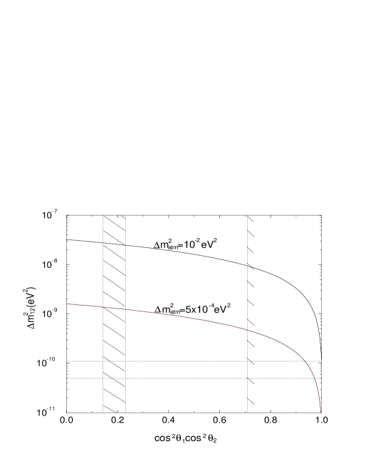
Figure 1: $\Delta m_{12}^{2}/{\rm eV}^{2}$ (solid lines) as a function of $c_{1}^{2}c_{2}^{2}$ for $\Delta m_{atm}^{2}=10^{-2}\,{\rm eV}^{2}$ (upper curve) and $5\times 10^{-4}\,{\rm eV}^{2}$ (lower). The experimentally allowed region for $c_{1}^{2}c_{2}^{2}$ is delimited by the dashed lines (the dashed regions are forbidden) and the $\Delta m_{sol}^{2}$ needed for the VO solution is given by the range between the dotted lines. This plot corresponds to the SM with $\Lambda=10^{3}\,{\rm GeV}$.

The precise results are given in Figure 1, which shows the predicted $\Delta m_{12}^{2}$ in ${\rm eV}^{2}$ (solid lines) as a function of $c_{1}^{2}c_{2}^{2}$ for the SM case with $\Lambda=10^{3}\,{\rm GeV}$ and $\Delta m_{atm}^{2}=5\times 10^{-4}\,{\rm eV}^{2}$ (lower curve) and $10^{-2}\,{\rm eV}^{2}$ (upper curve). The experimental constraints on $\theta_{1,2}$ leave open the windows $0\leq c_{1}^{2}c_{2}^{2}\leq 0.142$ and $0.232\leq c_{1}^{2}c_{2}^{2}\leq 0.71$, as indicated. The neutrino mass splitting required by VO solar oscillations is marked by the horizontal dotted lines. As was clear from the previous discussion, there is no overlapping between the $\Delta m_{12}^{2}$ predicted and the $\Delta m_{sol}^{2}$ required. Indeed, $\Delta m_{12}^{2}$ is always much larger than the allowed range. In the MSSM (or for larger $\Lambda$) the situation is even worse because in both cases $\Delta m_{12}^{2}$ increases significantly in the way discussed above.

Let us turn in more detail to the mixing angles in this scenario. At the scale $\Lambda$ one has some mixing angles $\theta_{i}$ which will be different in general at the scale $M_{Z}$ after radiative corrections to ${\cal M}_{\nu}$ have been included. At the same level of approximation as in Eqs. (8), the eigenvectors of the perturbed neutrino mass matrix are of the form

$$V_{1}^{\prime}=\frac{1}{\sqrt{\alpha^{2}+\beta^{2}}}(\alpha V_{1}+\beta V_{2}),\;\;\;V_{2}^{\prime}=\frac{1}{\sqrt{\alpha^{2}+\beta^{2}}}(-\beta V_{1}+\alpha V_{2}),\;\;\;V_{3}^{\prime}=V_{3},$$ (12)

where $V_{i}$ are the eigenvectors corresponding to ${\cal M}_{\nu}(\Lambda)$

$$V_{1}=\left(\begin{array}[]{c}c_{2}c_{3}\vspace{.1cm}\\ -c_{1}s_{3}-s_{1}s_{2}c_{3}\vspace{.1cm}\\ s_{1}s_{3}-c_{1}s_{2}c_{3}\end{array}\right),~{}~{}V_{2}=\left(\begin{array}[]{c}c_{2}s_{3}\vspace{.1cm}\\ c_{1}c_{3}-s_{1}s_{2}s_{3}\vspace{.1cm}\\ -s_{1}c_{3}-c_{1}s_{2}s_{3}\end{array}\right),~{}~{}V_{3}=\left(\begin{array}[]{c}s_{2}\vspace{.1cm}\\ s_{1}c_{2}\vspace{.1cm}\\ c_{1}c_{2}\end{array}\right).$$ (22)

From this, we deduce that the relationships between $\theta_{i}(M_{Z})$ and $\theta_{i}(\Lambda)$ are

$$\begin{array}[]{cl}\sin^{2}2\theta_{1}(M_{Z})=&\sin^{2}2\theta_{1}(\Lambda),\vspace{0.2cm}\\ \sin^{2}2\theta_{2}(M_{Z})=&\sin^{2}2\theta_{2}(\Lambda),\vspace{0.2cm}\\ \sin^{2}2\theta_{3}(M_{Z})=&\sin^{2}2\theta_{3}(\Lambda)+{\displaystyle\frac{2}{(1+r)^{2}}}\left[\sqrt{r}(1-r)\sin 4\theta_{3}(\Lambda)+2r\cos 4\theta_{3}(\Lambda)\right],\end{array}$$ (23)

where $r\equiv\alpha^{2}/\beta^{2}$. In leading-log approximation we have

$$\frac{\alpha}{\beta}\simeq\frac{s_{1}c_{3}+c_{1}s_{2}s_{3}}{s_{1}s_{3}-c_{1}s_{2}c_{3}},$$ (24)

with all angles evaluated at the scale $\Lambda$.

If we substitute this in (23) we find the simpler expression

$$\sin^{2}2\theta_{3}(M_{Z})=\frac{\sin^{2}\theta_{2}\sin^{2}2\theta_{1}}{(1-\cos^{2}\theta_{1}\cos^{2}\theta_{2})^{2}}.$$ (25)

For the bimaximal mixing case ($s_{2}\sim 0$, $c_{1}\sim s_{1}\sim 1/\sqrt{2}$) we end up with $\sin^{2}2\theta_{3}(M_{Z})\sim 0$, which is not acceptable (observations require $\sin^{2}2\theta_{3}\geq 0.67$).

In conclusion, the scenario $m_{1}\sim m_{2}\gg m_{3}$ is very contrived from the theoretical point of view. It is not natural to expect in this framework the values of mass splittings and mixing angles which are suggested by experiment. As mentioned in the Introduction, the only way-out would be an extremely artificial fine-tuning between the initial values of the mass splittings (and mixing angles) and the effect of the RG running. If one insists on this possibility, starting for example with ${\Delta m_{atm}^{2}=5\times 10^{-4}\ {\rm eV}^{2}}$, $s_{2}\sim 0$, $c_{1}\sim s_{1}\sim 1/\sqrt{2}$, $\Lambda=10^{3}$ GeV (a conservative choice for the fine-tuning problem), one is forced to take the initial mass splitting and mixing angle within the narrow ranges $|m_{1}^{2}-m_{2}^{2}|\sim(1.82\pm 0.02)\times 10^{-7}\,{\rm eV}^{2}$ and $\theta_{3}\sim\pi/2\pm 5.5\times 10^{-3}$ in order to compensate the effect of the RGEs and reproduce the required pattern of masses and mixings at $M_{Z}$ [these numbers cannot be extracted from the previous eq.(11), as in this case the approximation of initial degenerate eigenvalues does not hold]. One cannot certainly expect such a conspiracy between totally unrelated effects. If one slightly separates from these narrow ranges the low-energy mass splitting would be much larger than the required one. Of course, as $\Delta m_{atm}^{2}$ or $\Lambda$ are raised, or one goes to the supersymmetric case, the fine-tuning becomes much stronger.

Finally, it is interesting to note that for sizeable values of the cut-off ($\Lambda\stackrel{{\scriptstyle>}}{{{}_{\sim}}}10^{12}\ {\rm GeV}$) and/or a supersymmetric scenario, the values of $\Delta m_{12}^{2}$ are naturally 1-3 orders of magnitude larger than those represented in Fig.1, falling in the small-angle MSW range ($3\times 10^{-6}\ {\rm eV}^{2}<\Delta m^{2}_{sol}<10^{-5}\ {\rm eV}^{2}$). This is appealing since, as has been discussed in this section, starting with $\theta_{1,2}$ mixing angles in agreement with experiment ($s_{2}\sim 0$, $c_{1}\sim s_{1}\sim 1/\sqrt{2}$) the RGEs drive $\sin^{2}2\theta_{3}(M_{Z})\sim 0$, independently of its initial high-energy value, see eq.(23). This is exactly what is needed for a successful small-angle MSW solution to the solar neutrino problem.

2.2 $m_{1}\simeq-m_{2}$

In this case, the neutrino mass eigenvalues at $M_{Z}$ are, in leading-log approximation

$$\begin{array}[]{cl}m_{1}=&m_{\nu}\left[1+2\epsilon_{\tau}(s_{1}s_{3}-c_{1}s_{2}c_{3})^{2}\right],\vspace{0.2cm}\\ m_{2}=&-m_{\nu}\left[1+2\epsilon_{\tau}(s_{1}c_{3}+c_{1}s_{2}s_{3})^{2}\right],\vspace{0.2cm}\\ m_{3}=&0,\end{array}$$ (26)

with $\epsilon_{\tau}$ as given by Eqs. (9) and (10). The mixing angles are, in first approximation, equal at $M_{Z}$ and $\Lambda$. We fix again $m_{\nu}\sim\sqrt{\Delta m_{atm}^{2}}$. In order not to spoil the size of the required solar mass splitting, the radiative corrections should generate $\Delta m_{12}^{2}\leq\Delta m_{sol}^{2}$. The prediction from (26) is

$$\frac{\Delta m_{12}^{2}}{m_{\nu}^{2}}=\frac{\Delta m_{12}^{2}}{\Delta m_{atm}^{2}}=4\epsilon_{\tau}\left[(\cos^{2}\theta_{1}\sin^{2}\theta_{2}-\sin^{2}\theta_{1})\cos 2\theta_{3}-\sin 2\theta_{1}\sin\theta_{2}\sin 2\theta_{3}\right].$$ (27)

Getting a sufficiently small number for this quantity requires some (in general delicate) correlation between the mixing angles, in such a way that

$$\tan 2\theta_{3}\simeq\frac{\cos^{2}\theta_{1}\sin^{2}\theta_{2}-\sin^{2}\theta_{1}}{\sin\theta_{2}\sin 2\theta_{1}}.$$ (28)

It is remarkable that the bimaximal values of the mixing angles ($\sin^{2}2\theta_{1}\sim\sin^{2}2\theta_{3}\sim 1$ and $\sin^{2}2\theta_{2}\sim 0$) do satisfy (28).

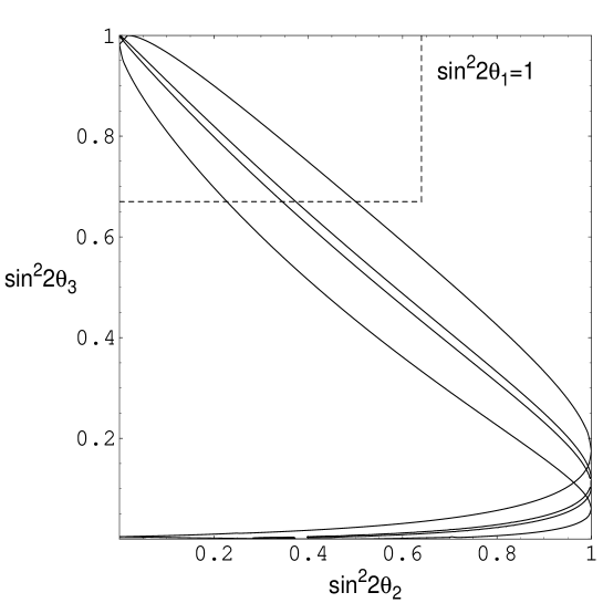
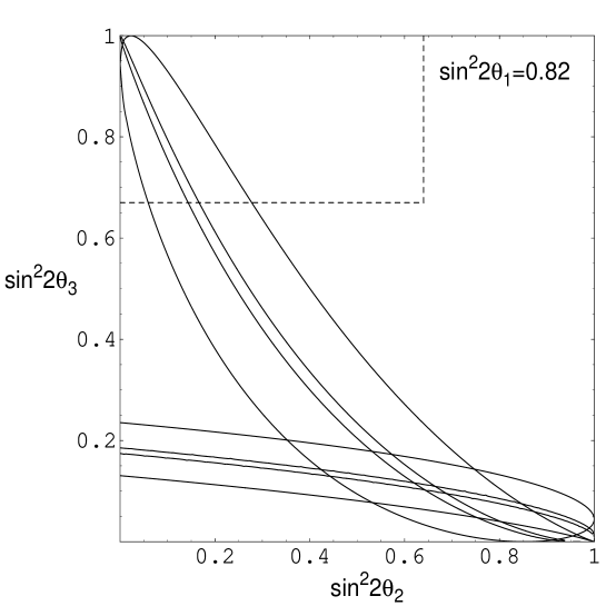
Figure 2: Allowed regions (in which $\Delta m_{12}^{2}\leq 1.1\times 10^{-10}\,{\rm eV}^{2}$) in the plane ($\sin^{2}2\theta_{2},\sin^{2}2\theta_{3}$) for the SM case for $\sin^{2}2\theta_{1}=1$ (upper plot) and 0.82 (lower). The area between the outermost (innermost) lines corresponds to a cut-off scale $\Lambda=10^{3}\,{\rm GeV}$ ($10^{12}\,{\rm GeV}$). The dashed lines delimit the experimentally allowed values for $\sin^{2}2\theta_{2}$ and $\sin^{2}2\theta_{3}$.

Figures 2a,b show, for the SM case, the regions in the plane $(\sin^{2}2\theta_{2},\sin^{2}2\theta_{3})$ where the correlation (28) takes place, giving $\Delta m_{12}^{2}\leq 1.1\times 10^{-10}\,{\rm eV}^{2}$ (the upper limit on $\Delta m^{2}_{sol}$). The width of these allowed regions is controlled by $\Delta m_{sol}^{2}/(\epsilon_{\tau}\Delta m_{atm}^{2})$. The larger $\epsilon_{\tau}\Delta m_{atm}^{2}$ (or the smaller $\Delta m^{2}_{sol}$), the thinner these regions get [because a more delicate cancellation must take place in (28)]. In figure 2a we have fixed $\sin^{2}2\theta_{1}=1$ and $\Delta m_{atm}^{2}=5\times 10^{-4}\,{\rm eV}^{2}$, and we give the allowed areas for the two choices $\Lambda=10^{3}\,{\rm GeV}$ (thick region, delimited by the outermost lines) and $10^{12}\,{\rm GeV}$ (thin region). If we choose $\Delta m_{atm}^{2}=10^{-2}\,{\rm eV}^{2}$ instead, the two regions would shrink significantly and will be somewhere inside the thin region shown for $\Lambda=10^{12}\,{\rm GeV}$. The dashed lines delimit the allowed region for the two mixing angles $\theta_{2}$ and $\theta_{3}$ ($0\leq\sin^{2}2\theta_{2}\leq 0.64$ and $0.67\leq\sin^{2}2\theta_{3}\leq 1$). Figure 2b corresponds to the case $\sin^{2}2\theta_{1}=0.82$ (the lower experimental limit) and the same values of other parameters as in figure 2a. The results are similar except for a shift towards smaller $\sin^{2}2\theta_{2}$ values in the region of interest. Note in particular that the upper limit $\sin^{2}2\theta_{2}\sim 0.64$ is never reached in this scenario. We see that in the most conservative case, with $\Delta m_{atm}^{2}=5\times 10^{-4}\,{\rm eV}^{2}$ and $\Lambda=10^{3}\,{\rm GeV}$, a significant portion of parameter space could accommodate a $\Delta m_{12}^{2}$ of the right order of magnitude (including the bimaximal mixing solution). It is interesting to note that inside this region, starting with degenerate $m_{1},\ m_{2}$ would lead to a correct $\Delta m_{sol}^{2}$ at low energy, thus providing a dynamical origin for this small number. Notice however that as soon as $\Delta m_{atm}^{2}$ or $\Lambda$ are raised the required fine-tuning becomes much stronger. This occurs in particular if the lower bound $\Delta m_{atm}^{2}=5\times 10^{-4}$ that we have used is increased according to the analyses of the most recent data [11].

The situation is worse in the MSSM case. Roughly speaking, for $\tan\beta=3$ radiative corrections are 20 times larger than in the SM (with the same $\Lambda$). The cancellation between mixing angles in (28) is thus much more delicate in the supersymmetric case, as expected.

3 Conclusions

The vacuum oscillation (VO) solution to the solar neutrino problem requires an extremely small mass splitting, $\Delta m^{2}_{sol}\stackrel{{\scriptstyle<}}{{{}_{\sim}}}10^{-10}\ {\rm eV}^{2}$. We have studied in this paper under which circumstances this smallness (whatever its origin) is or is not spoiled by radiative corrections, in particular by the running of the renormalization group equations (RGEs) between the scale at which the effective neutrino mass matrix is generated ($\Lambda$) and low energy. We consider the cases where the effective theory below $\Lambda$ is the Standard Model (SM) or the Minimal Supersymmetric Standard Model (MSSM). The results depend dramatically on the type of neutrino spectrum. In particular, if $m_{1}^{2}\ll m_{2}^{2}\ll m_{3}^{2}$, radiative corrections are always relatively small and do not cause any significant change in the splittings. On the other hand, if $m_{1}^{2}\sim m_{2}^{2}\sim m_{3}^{2}$, radiative corrections always induce mass splittings that are several orders of magnitude larger than the required $\Delta m^{2}_{sol}$. Hence, this type of spectrum is not plausible for the VO solution. The only way-out would be an extremely artificial fine-tuning between the initial values of the mass splittings (and mixing angles) and the effect of the RG running, something clearly unacceptable.

Most of the paper is devoted to the third possible type of spectrum, $m_{1}^{2}\sim m_{2}^{2}\gg m_{3}^{2}$, which requires $m_{1,2}^{2}\sim\Delta m^{2}_{atm}$ (or larger). Here again, the radiatively generated splittings are in general too large, making the scenario unnatural. As a general rule, this gets worse as $\Delta m_{atm}^{2}$ or $\Lambda$ grow. Also, the supersymmetric scenario works worse than the SM one, especially as $\tan\beta$ incresases. More precisely, if $m_{1}$ and $m_{2}$ have equal signs, the RGE-induced splittings are always too large, even for the most favorable case. In addition, the solar mixing angle is driven by the RGEs to very small values, $\sin^{2}2\theta_{3}(M_{Z})\sim 0$, which is incompatible with the VO solution. It is however worth noticing that such a small angle is what is needed for a successful small-angle MSW solution to the solar neutrino problem. Moreover, for $\Lambda\stackrel{{\scriptstyle>}}{{{}_{\sim}}}10^{12}\ {\rm GeV}$ and/or for the MSSM scenario the values of $\Delta m_{12}^{2}$ may fall naturally in the small-angle MSW range, $\sim 10^{-5}\ {\rm eV}^{2}$.

If $m_{1}$ and $m_{2}$ have opposite signs, the results are analogous, but now the splitting generated by the RGEs can vanish if the mixing angles are correlated in a particular way (which remarkably is always satisfied by the exact bimaximal case). This correlation or tuning of parameters is acceptable in the SM scenario, provided the cut-off scale $\Lambda$ is not much larger than $\sim 1\,{\rm TeV}$ and if $\Delta m_{atm}^{2}$ is in the low side of its experimentally preferred range ($\sim 5\times 10^{-4}\,{\rm eV}^{2}$). Interestingly, this could provide a dynamical origin for the smallness of $\Delta m^{2}_{sol}$. For larger $\Lambda$ and/or $\Delta m_{atm}^{2}$ (or equivalently, for the MSSM scenario) radiative corrections grow in size and the required tuning of mixing angles becomes quickly unacceptable. This occurs in particular if the lower bound $\Delta m_{atm}^{2}=5\times 10^{-4}$ that we have used is increased according to the most recent data analyses [11].

In conclusion, apart from the mentioned small windows, a completely hierarchical spectrum of neutrinos (i.e. as the spectrum of quarks and charged leptons), $m_{1}^{2}\ll m_{2}^{2}\ll m_{3}^{2}$, seems to be the only plausible one for the VO solution to the solar neutrino problem.

References

• [1] R. Barbieri et al., JHEP 9812 (1998) 017; G.L. Fogli, E. Lisi, A. Marrone and G. Scioscia, Phys. Rev. D59:033001 (1999), [hep-ph/9904465].
• [2] Y. Fukuda et al., Super-Kamiokande Collaboration, Phys. Lett. B433 (1998) 9; Phys. Rev. Lett. 81 (1998) 1562; S. Hatakeyama et al., Kamiokande Collaboration, Phys. Rev. Lett. 81 (1998) 2016.
• [3] First ref. in [1]; A. Strumia, JHEP 9904 (1999) 026.
• [4] Y. L. Wu, [hep-ph/9810491], [hep-ph/9901245] and [hep-ph/9901320]; C. Wetterich, Phys. Lett. B451 (1999) 397; R. Barbieri, L.J. Hall, G.L. Kane, and G.G. Ross, [hep-ph/9901228]; M. Tanimoto, T. Watari, T. Yanagida, [hep-ph/9904338].
• [5] S. Weinberg, Phys. Rev. Lett. 43 (1979) 1566.
• [6] K. Babu, C. N. Leung and J. Pantaleone, Phys. Lett. B319 (1993) 191.
• [7] G. Altarelli and F. Feruglio, Phys. Lett. B439 (1998) 112, JHEP 9811 (1998) 021 , and Phys. Lett. B451 (1999) 388.
• [8] J. Ellis and S. Lola, [hep-ph/9904279].
• [9] J.A. Casas, J.R. Espinosa, A. Ibarra and I. Navarro, [hep-ph/9904395].
• [10] J.A. Casas, J.R. Espinosa, A. Ibarra and I. Navarro, [hep-ph/9905381].
• [11] K. Scholberg, [hep-ex/9905016].