Semi-Inclusive Hadron Production at HERA: the Effect of QCD Gluon Resummation

Abstract

We present a formalism that improves the applicability of perturbative QCD in the current region of semi-inclusive deep inelastic scattering. The formalism is based on all-order resummation of large logarithms arising in the perturbative treatment of hadron multiplicities and energy flows in this region. It is shown that the current region of semi-inclusive DIS is similar to the region of small transverse momenta in vector boson production at hadron colliders. We use this resummation formalism to describe transverse energy flows and charged particle multiplicity measured at the electron-proton collider HERA. We find good agreement between our theoretical results and experimental data for the transverse energy flows.

I Introduction

It is well known that perturbative Quantum Chromodynamics (pQCD) is a very powerful but not omnipotent theory of the strong interactions of elementary particles. It can be successfully applied to the calculation of various physical observables whenever the kinematics of the particle interaction process implies the existence of a large scale $Q$ with dimensionality of momentum. For such a kinematic regime, the cross-section of the hadronic process can be represented as a convolution of the perturbatively calculable hard part, describing the energetic short-range interactions of hadronic constituents (partons), and several process-independent nonperturbative functions, relevant to the complicated strong dynamics at large distances.

The factorization of the hard and soft parts has proven to be a powerful method for the calculation of hadronic scattering cross-sections. Unfortunately, near the boundaries of the kinematic phase space the convergence of the perturbative solution can be spoiled by the presence of large logarithms $\log r$, where $r$ is some dimensionless function of the kinematic parameters of the system. For instance, $r$ might be a small ratio of two momentum scales $P_{1}$ and $P_{2}$ of the system, $r=P_{1}/P_{2}$.

To handle this situation, techniques for the all-order resummation of the logarithmically divergent terms have been developed [1, 2, 3, 4, 5, 13]. These techniques have been successfully used to improve the applicability of perturbative QCD in several processes (calculation of energy correlations in $e^{+}e^{-}$ annihilation [4], transverse momentum distributions in vector boson [5, 20, 21, 22],di-photon [6] and Higgs [7] production at hadron colliders).

In this paper, we will consider another process, the production of hadrons in deep-inelastic lepton-hadron scattering (DIS). As will be discussed below, some features of this process are similar to the $e^{+}e^{-}$ hadroproduction and vector boson production, so that in certain kinematic regions the description of this process requires all-order resummation of the large logs which would otherwise spoil the convergence of the perturbative calculation.

Deep-inelastic lepton-hadron scattering (DIS) at large momentum transfer $Q$ is one of the cornerstone processes to test pQCD. Traditionally, the experimental study of the fully inclusive DIS process, $e+A\rightarrow e+X$ where $A$ is usually a nucleon, and $X$ is any final state, is used to obtain information about the Parton Distribution Functions of the nucleon (PDFs). These functions describe the long-range dynamics of hadron interactions, and are required by many pQCD calculations.

During the 1990’s, significant attention has also been paid to various aspects of semi-inclusive deep inelastic scattering (semi-inclusive DIS), for instance, the semi-inclusive production of hadrons and jets, $e+A\rightarrow e+B+X$ and $e+A\rightarrow e+jets+X$. In particular, the H1 and ZEUS collaborations at HERA, and the E665 experiment at Fermilab performed extensive experimental studies of the charged particle multiplicity [8, 9, 10] and hadronic transverse energy flows [11] at large momentum transfer $Q$. It was found that some aspects of the data, e.g., the Feynman $x$ distributions, can be successfully explained in the framework of perturbative QCD analysis [12]. On the other hand, the applicability of pQCD for the description of other features of the process is limited. For example, the perturbative calculation in lowest orders fails to describe the pseudorapidity or transverse momentum distributions of the final hadrons. Under certain kinematic conditions the whole perturbative expansion as a series in the QCD coupling may fail due to the large logarithms mentioned earlier.

To be more specific, consider semi-inclusive DIS production of hadrons of a type $B$. At large energies, we can neglect the masses of the participating particles. In semi-inclusive DIS at given energies of the beams, any event can be characterized by two energy scales: the virtuality of the exchanged photon $Q$ and the scale $q_{T}$ related to the transverse momentum of the final hadron $B$. The exact definition of $q_{T}$ will be given in the main part of the paper. One may try to use pQCD in any of three regions, where $Q$, $q_{T}$, or both $Q$ and $q_{T}$ are large. The renormalization and factorization scales should be chosen to be of the order of the large physical scale of the process. In the limit $Q\ll q_{T}$ (photoproduction region) pQCD may fail due to the large terms $(\log Q/q_{T})^{n}$ as $Q\rightarrow 0$, which should be resummed into the parton distribution function of the virtual photon [16]. The limit $Q\gg q_{T}$ is similar to the limit of a small transverse momentum in vector boson production where logarithms of the type $(\log q_{T}/Q)^{n}$ should be resummed in order to get a finite cross-section of the process [5]. Finally, in the region $q_{T}\approx Q$ one may encounter another type of large logarithms corresponding to events with large rapidity gaps $\Delta y$. This type of large logarithms can be resummed with the help of the Balitsky-Fadin-Kuraev-Lipatov (BFKL) formalism[13].

The purpose of this paper is to discuss the resummation of large logarithms in semi-inclusive DIS hadroproduction $e+A\rightarrow e+B+X$ in the limit $q_{T}\ll Q$. These are large logs arising from to the emission of soft and collinear partons, which we resum using the formalism of Collins, Soper, and Sterman (CSS) [5]. Our calculations are based on the works of Meng, Olness, and Soper  [14, 15], who analyzed the resummation technique for a particular energy distribution function of the semi-inclusive DIS process. This energy distribution function receives contributions from all possible final state hadrons, and does not depend on the specifics of fragmentation in the final state.

In this paper we present a more general formalism than the one developed in [14, 15], which will also account for the final state fragmentation of the partons. This formalism requires the knowledge of the fragmentation functions (FFs) describing nonperturbative fragmentation of final partons into observed hadrons. Correspondingly, this formalism can consider a wider class of physical observables including particle multiplicities. Our calculations will be done in the next-to-leading order of perturbative QCD. As an example of a practical application of our formalism, we compare our calculation with the H1 data on the pseudorapidity distributions of the transverse energy flow [11] in the $\gamma^{*}p$ center-of-mass frame. We also present predictions for charged particle multiplicity. Another goal of this study is to find in which regions of kinematic parameters the CSS resummation formalism is sufficient to describe the existing data, and in which regions significant contributions from other hadroproduction mechanisms, such as the BFKL interactions [13], higher order corrections including multijet production with [16] or without [17] resolved photon contributions, or photoproduction showering [18], cannot be ignored.

The outline of the paper is as follows. In Section II we define the kinematic variables for the semi-inclusive DIS process and specify the coordinate frames which will be used throughout the following discussion. In Section III we derive the resummed cross-section formulas. In Section IV we extend the results of Section III to obtain the resummed energy flows. In Section V we describe the matching between the resummed and perturbative cross-sections and energy flows. We also discuss kinematic corrections, which should be applied to the resummed cross-section to account for fast contraction of the phase space of the perturbative cross-section at $q_{T}\approx Q$. In Section VI we describe the results of Monte Carlo calculations for the resummed cross-sections and energy flows. We present the comparison of our calculation with the existing energy flow data from HERA. We also suggest how one can reanalyze the existing HERA and Fermilab-E665 data on charged particle production in order to adapt it for unambiguous extraction of the non-perturbative Sudakov factors.

II Kinematic Variables

We follow notations which are similar to the ones used in [14, 15]. In this Section we summarize them.

We limit the discussion to the case of semi-inclusive DIS at the $ep$ collider HERA. We consider the process

$$e+A\rightarrow e+B+X,$$ (1)

where $e$ is an electron or positron, $A$ is a proton, $B$ is a hadron observed in the final state, and $X$ represents any other particles in the final state in the sense of inclusive scattering (Fig. 1). We denote the momenta of $A$ and $B$ by $p_{A}^{\mu}$ and $p_{B}^{\mu}$, and the momenta of the lepton in the initial and final states by $l^{\mu}$ and $l^{\prime\mu}$. Also, $q^{\mu}$ is the momentum transfer to the hadron system, $q^{\mu}=l^{\mu}-{\l^{\prime}}^{\mu}$. For most of this paper, until the discussion of charged particle multiplicity, we will neglect the particle masses.

FIG. 1.: Semi-inclusive deep inelastic scattering

We assume that the initial lepton and hadron interact only through a single photon exchange. Therefore, $q^{\mu}$ also has the meaning of the 4-momentum of the exchanged virtual photon $\gamma^{*}$.

A Lorentz scalars

For further discussion, we define five Lorentz scalars relevant to the process (1). The first is the center-of-mass energy of the initial hadron and lepton $\sqrt{S_{eA}}$ where

$$S_{eA}=(p_{A}+l)^{2}=2p_{A}\cdot l.$$ (2)

We will also use the conventional DIS variables $x$ and $Q^{2}$ which are defined from the momentum transfer $q^{\mu}$ by

$$Q^{2}=-q^{2}=2\ell\cdot\ell^{\prime},$$ (3)

$$x=\frac{Q^{2}}{2p_{A}\cdot{q}}\ .$$ (4)

In principle, $x$ and $Q^{2}$ can be completely determined in an experimental event by measuring the momentum of the outgoing lepton.

Next we define a scalar $z$ related to the momentum of the final hadron state $B$ by

$$z=\frac{p_{B}\cdot p_{A}}{q\cdot p_{A}}=\frac{2xp_{B}\cdot p_{A}}{Q^{2}}~{}.$$ (5)

The variable $z$ plays an important role in the description of fragmentation in the final state. In particular, in the quark-parton model (or in the leading order perturbative calculation) it is equal to the fraction of the fragmenting parton’s momentum carried away by the observed hadron.

The next relativistic invariant $q_{T}^{2}$ is the square of the component of the virtual photon’s 4-momentum $q^{\mu}$ that is transverse to the 4-momenta of the initial and final hadrons:

$$q_{T}^{2}=-q_{t}^{\mu}q_{t\mu},$$ (6)

where

$$q_{t}^{\mu}=q^{\mu}-p_{A}^{\mu}\frac{q\cdot p_{B}}{p_{A}\cdot p_{B}}-p_{B}^{\mu}\frac{q\cdot p_{A}}{p_{A}\cdot p_{B}}.$$ (7)

The orthogonality of $q_{t}^{\mu}$ to both $p_{A}^{\mu}$ and $p_{B}^{\mu}$, that is $q_{t}\cdot p_{A}=q_{t}\cdot p_{B}=0$, follows immediately from its definition (7).

The variable $q_{T}$ plays the same role in the semi-inclusive DIS resummation as the transverse momentum of a vector boson in resummation of vector boson production at hadron colliders. In particular, the theoretical cross-section calculated in a fixed order of pQCD is divergent in the limit $q_{T}\rightarrow 0$, so that all-order resummation is needed to make the predictions of the theory finite in this limit.

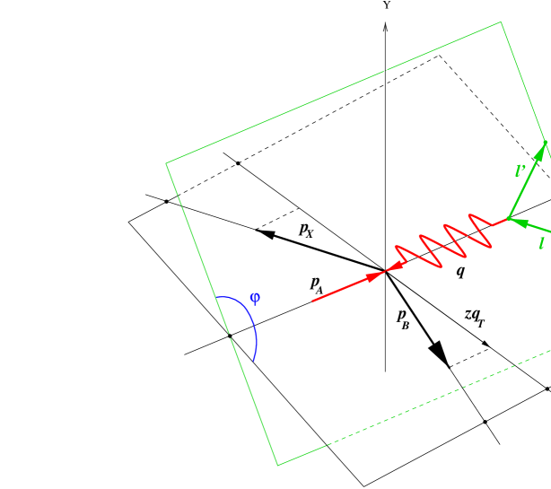
FIG. 2.: Geometry of the particle momenta in the hadron frame

In the analysis of kinematics, we will use two reference frames. The first is the center-of-mass (c.m.) frame of the initial hadron and the virtual photon. The second is a special type of Breit frame which we will call, depending on whether the initial state is a hadron or a parton, the hadron or parton frame. As was shown in [14, 15], by using the hadron frame one can organize the resummation formalism for semi-inclusive DIS in a way that is similar to the case of vector boson production. On the other hand, many experimental results are presented in the $\gamma^{*}p$ c.m. frame. We will use a subscript $h$ and $cm$ to denote kinematic variables in the hadron or c.m. frame.

B Hadron frame

Following Meng et al. [14, 15] the hadron frame is defined by two conditions: (a) the 4-momentum of the virtual photon is purely space-like, and (b) the momentum of the outgoing hadron $B$ lies in the $xz$ plane. The directions of particle momenta in this frame are shown in Fig. 2.

In this frame the proton $A$ moves in the $+z$ direction, while the momentum transfer $\vec{q}$ is in the $-z$ direction, and $q^{0}$ is 0:

$$q^{\mu}_{h}=(0,0,0,-Q),$$ (8)

$$p_{A,h}^{\mu}=\frac{Q}{2x}\Bigl{(}1,0,0,1\Bigr{)}.$$ (9)

The momentum of the final-state hadron $B$ is

$$p_{B,h}^{\mu}=\frac{zQ}{2}\Bigl{(}1+\frac{q_{T}^{2}}{Q^{2}},\frac{2q_{T}}{Q},0,\frac{q_{T}^{2}}{Q^{2}}-1\Bigr{)}.$$ (10)

The incoming and outgoing lepton momenta in the hadron frame are defined in terms of variables $\psi$ and $\phi$ as follows [19]:

$$\ell^{\mu}_{h}=\frac{Q}{2}(\cosh\psi,\sinh\psi\cos\phi,\sinh\psi\sin\phi,-1),$$ (11)

$$\ell^{\prime\mu}_{h}=\frac{Q}{2}(\cosh\psi,\sinh\psi\cos\phi,\sinh\psi\sin\phi,+1).$$ (12)

Note that $\phi$ is the azimuthal angle of $\vec{\ell}_{h}$ or $\vec{\ell}^{\prime}_{h}$ around the $z$-axis. $\psi$ is a parameter of a boost which relates the hadron frame to a lepton Breit frame in which $\ell^{\mu}=(Q/2,0,0,-Q/2)$. By (2) and (11) we find that

$$\cosh\psi=\frac{2xS_{eA}}{Q^{2}}-1=\frac{2}{y}-1,$$ (13)

where the conventional DIS variable $y$ is defined as

$$y=\frac{Q^{2}}{xS_{eA}}.$$ (14)

The allowed range of the variable $y$ in deep-inelastic scattering is $0\leq y\leq 1$; therefore $\psi\geq 0$.

The transverse part of the virtual photon momentum $q_{t}^{\mu}$ has a simple form in the hadron frame; it can be shown that

$$q_{t,h}^{\mu}=(-\frac{q_{T}^{2}}{Q},-q_{T},0,-\frac{q_{T}^{2}}{Q})~{}.$$ (15)

In other words, $q_{T}$ is the magnitude of the transverse component of $\vec{q}_{t,h}$. The transverse momentum $p_{T}$ of the final state hadron $B$ in this frame is simply related to $q_{T}$, by

$$p_{T}=zq_{T}.$$ (16)

Also, the pseudorapidity of $B$ in the hadron frame is

$$\eta_{h}\equiv-\log\Bigl{(}\tan\frac{\theta_{B,h}}{2}\Bigr{)}=\log\frac{q_{T}}{Q}.$$ (17)

The resummed cross-section will be derived using the hadron frame. To transform the result to other frames, it is useful to express the basis vectors of the hadron frame ($T^{\mu},\ X^{\mu},\ Y^{\mu},\ Z^{\mu}$) in terms of the particle momenta [14]. For an arbitrary coordinate frame,

$$T^{\mu} = \frac{q^{\mu}+2xp_{A}^{\mu}}{Q},$$ (18)

$$X^{\mu} = \frac{1}{q_{T}}\Biggl{(}\frac{p^{\mu}_{B}}{z}-q^{\mu}-\Bigl{[}1+\frac{q_{T}^{2}}{Q^{2}}\Bigr{]}xp_{A}^{\mu}\Biggr{)},$$ (19)

$$Y^{\mu} = \epsilon^{\mu\nu\rho\sigma}Z_{\nu}T_{\rho}X_{\sigma},$$ (20)

$$Z^{\mu} = -\frac{q^{\mu}}{Q}.$$ (21)

If these relations are evaluated in the hadron frame, the basis vectors $T^{\mu},\ X^{\mu},\ Y^{\mu},\ Z^{\mu}$ are $(1,0,0,0),\ (0,1,0,0),(0,0,1,0),(0,0,0,1)$, respectively.

The relationships between the hadron-frame variables and the HERA lab-frame momenta are presented in Appendix A.

C Photon-hadron center-of-mass frame

The center-of-mass frame of the proton $A$ and virtual photon $\gamma^{*}$ is defined by the condition $\vec{p}_{A,cm}+\vec{q}_{cm}=0$. The relationship between particle momenta in this frame is illustrated in Fig. 3. As in the hadron frame, the momenta $\vec{q}_{cm}$ and $\vec{p}_{A,cm}$ in the c.m. frame are directed along the $z$ axis. The coordinate transformation from the hadron frame into the $\gamma^{*}p$ c.m. frame consists of (a) a boost in the direction of the virtual photon and (b) inversion of the direction of the $z$ axis, which is needed to make the definition of the c.m. frame consistent with the one adopted in HERA experimental publications. In the c.m. frame the momentum of $\gamma^{*}$ is

$$q_{cm}^{\mu}=\Biggl{(}\frac{W^{2}-Q^{2}}{2W},0,0,\frac{W^{2}+Q^{2}}{2W}\Biggr{)},$$ (22)

where $W$ is the c.m. energy of the $\gamma^{*}p$ collisions,

$$W^{2}=(p_{A}+q)^{2}.$$ (23)

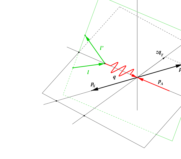
FIG. 3.: Particle momenta in the $\gamma^{*}p$ c.m. frame

The momenta of the initial and final hadrons $A$ and $B$ are given by

$$p^{\mu}_{A,cm}=\Biggl{(}\frac{W^{2}+Q^{2}}{2W},0,0,-\frac{W^{2}+Q^{2}}{2W}\Biggr{)},$$ (24)

$$p^{\mu}_{B,cm}=\Biggl{(}E_{B},p_{B,cm}\sin\theta^{cm}_{B},0,p_{B,cm}\cos\theta^{cm}_{B}\Biggr{)}.$$ (25)

Since the hadron and c.m. frames are related by a boost along the $z$-direction, the expression for the transverse momentum of the final hadron $B$ in the c.m. frame is the same as the one in the hadron frame,

$$p_{T}=zq_{T}.$$ (26)

Also, similar to the case of the hadron frame, the relationship between $q_{T}$ and the pseudorapidity of $B$ in the c.m. frame is simple,

$$q_{T}=We^{-\eta_{cm}}.$$ (27)

The limit of small $q_{T}$, which is most relevant for our resummation calculation, corresponds to the region of large pseudorapidities in the hadronic c.m. frame. Since in this case the final parton is produced in the direction of the momentum of the virtual photon, the region of large $\eta^{cm}$ is also called the current region.

D Parton kinematics

The kinematic variables and momenta discussed so far are all laboratory variables. Next, we relate these to parton variables.

Let $a$ denote the parton in $A$ that participates in the hard scattering, with momentum $p_{a}^{\mu}=\xi_{a}p_{A}^{\mu}$. Let $b$ denote the parton of which $B$ is a fragment, with momentum $p_{b}^{\mu}=p_{B}^{\mu}/\xi_{b}$. The momentum fractions $\xi_{a}$ and $\xi_{b}$ range from 0 to 1. At the parton level, we introduce the Lorentz scalars $\hat{x},\ \hat{z},\ \hat{q}_{T}$ analogous to the ones at the hadron level:

$$\hat{x}=\frac{Q^{2}}{2p_{a}\cdot{q}}=\frac{x}{\xi_{a}},$$ (28)

$$\hat{z}=\frac{p_{b}\cdot p_{a}}{q\cdot p_{a}}=\frac{z}{\xi_{b}},$$ (29)

$$\hat{q}_{T}^{2}=-\hat{q}_{t}^{\mu}\hat{q_{t}}_{\mu}.$$ (30)

Here $\hat{q}_{T}^{\mu}$ is the component of $q^{\mu}$ which is orthogonal to the parton 4-momenta $p^{\mu}_{a}$ and $p^{\mu}_{b}$,

$$\hat{q}_{t}\cdot p_{a}=\hat{q}_{t}\cdot p_{b}=0.$$

Therefore,

$$\hat{q}_{t}^{\mu}=q^{\mu}-p_{a}^{\mu}\frac{q\cdot p_{b}}{p_{a}\cdot p_{b}}-p_{b}^{\mu}\frac{q\cdot p_{a}}{p_{a}\cdot p_{b}}.$$ (31)

In the case of massless initial and final hadrons the hadronic and partonic $q_{T}$’s coincide,

$$\hat{q}_{T}=q_{T}.$$ (32)

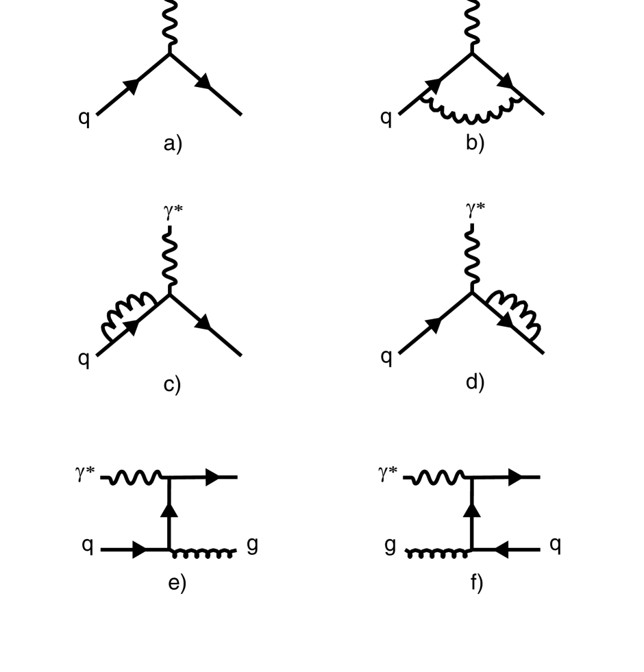
FIG. 4.: Feynman diagrams for semi-inclusive DIS: a) LO; b-d)NLO virtual diagrams; e-f) NLO real emission diagrams

III The resummed NLO cross-section

The knowledge of five Lorentz scalars $S_{eA},\ Q,\ q_{T},\ x,\ z$ and the lepton azimuthal angle $\phi$ in the hadron frame is sufficient to specify unambiguously the kinematics of the semi-inclusive scattering event $e+A\rightarrow e+B+X$. In the following, we will discuss the hadron cross-section $d\sigma_{BA}$, which is related to the parton cross-section $d\hat{\sigma}_{ba}$ by

$$\frac{d\sigma_{BA}}{dxdzdQ^{2}dq_{T}^{2}d\phi}=\sum_{a,b}\int_{z}^{1}\frac{d\xi_{b}}{\xi_{b}}D_{B/b}(\xi_{b},\mu_{D})\int_{x}^{1}\frac{d\xi_{a}}{\xi_{a}}F_{a/A}(\xi_{a},\mu_{F})\frac{d\hat{\sigma}_{ba}}{d\hat{x}d\hat{z}dQ^{2}dq_{T}^{2}d\phi}.$$ (33)

Here $F_{a/A}(\xi_{a},\mu_{F})$ denotes the distribution function (PDF) of the parton of a type $a$ in the hadron $A$, and $D_{B/b}(\xi_{b},\mu_{D})$ is the fragmentation function (FF) for parton type $b$ and final hadron $B$. The parameters $\mu_{F}$ and $\mu_{D}$ are the factorization scales for the PDFs and FFs. In the following discussion and calculations, we assume that these factorization scales and the renormalization scale $\mu_{R}$ are the same,

$$\mu_{F}=\mu_{D}=\mu_{R}\equiv\mu.$$

The analysis of semi-inclusive DIS can be conveniently organized by separating the dependence of the parton and hadron cross-sections on the leptonic angle $\phi$ and the boost parameter $\psi$ from the other kinematic variables $x,\ z,\ Q$ and $q_{T}$ [19]. Following [14], we express the hadron (or parton) cross-section as a sum over products of functions of these lepton angles in the hadron frame $A_{\alpha}(\psi,\phi)$, and structure functions $V^{(\alpha)}_{BA}(x,z,Q^{2},q_{T}^{2})$ (or $\hat{V}^{(\alpha)}_{ba}(\hat{x},\hat{z},Q^{2},q_{T}^{2})$, respectively):

$$\frac{d\sigma_{BA}}{dxdzdQ^{2}dq_{T}^{2}d\phi}=\sum_{\alpha=1}^{4}V^{(\alpha)}_{BA}(x,z,Q^{2},q_{T}^{2})A_{\alpha}(\psi,\phi),$$ (34)

$$\frac{d\hat{\sigma}_{ba}}{d\hat{x}d\hat{z}dQ^{2}dq_{T}^{2}d\phi}=\sum_{\alpha=1}^{4}\hat{V}^{(\alpha)}_{ba}(\hat{x},\hat{z},Q^{2},q_{T}^{2})A_{\alpha}(\psi,\phi).$$ (35)

At the energy of HERA, hadroproduction via parity-violating $Z$-boson exchanges can be neglected, and only four out of the nine angular functions listed in [14] contribute to the cross-sections (34-35). They are

$$A_{1} = 1+\cosh^{2}\psi,$$ (36)

$$A_{2} = -2,$$ (37)

$$A_{3} = -\cos\phi\sinh 2\psi,$$ (38)

$$A_{4} = \cos 2\phi\sinh^{2}\psi.$$ (39)

We will assume that the angle $\phi$ is not monitored in the experiment, so that it will be integrated out in the following discussion. Correspondingly, our numerical result for $d\sigma/(dxdzdQ^{2}dq_{T}^{2})$ will not depend on terms in (34-35) proportional to the angular functions $A_{3}$ and $A_{4}$, which integrate to zero.

Out of the four structure functions, only $\hat{V}^{(1)}_{ba}$ receives contributions from both leading and next-to-leading order diagrams. Also, only the $\hat{V}^{(1)}_{ba}$ structure function diverges in the limit $q_{T}\rightarrow 0$.

The leading order (LO) parton process is $e+a\rightarrow e+b$ where the initial parton $a$ is a quark from the proton and the final quark $b$ (which is the same as $a$) fragments into the hadron $B$. The Feynman diagram for this process is shown in Fig. 4a. There is no LO contribution to semi-inclusive DIS from gluons.

The next-to-leading order (NLO) corrections are shown in Figs. 4b-f. At this order, we need to account for the virtual corrections to the LO subprocess $\stackrel{{\scriptstyle(-)}}{{q}}\gamma^{*}\rightarrow\stackrel{{\scriptstyle(-)}}{{q}}$ (Figs. 4b-d), as well as for the diagrams describing the subprocesses $\stackrel{{\scriptstyle(-)}}{{q}}\gamma^{*}\rightarrow\stackrel{{\scriptstyle(-)}}{{q}}g$ and $g\gamma^{*}\rightarrow q\bar{q}$, with the subsequent fragmentation of the final-state quark, antiquark or gluon (Figs. 4e-f).

Conservation of total 4-momentum in the real emission subprocesses (Figs. 4e-f) allows us to write the momentum of the unobserved final state parton (e.g. the gluon in Fig. 4e) as

$$p_{g}^{\mu}=q^{\mu}+p_{a}^{\mu}-p_{b}^{\mu}.$$ (40)

When there is no gluon radiation ($p_{g}^{\mu}=0$) the momentum of $b$ is $p_{b}^{\mu}=p_{a}^{\mu}+q^{\mu}$, and, according to (31), $q_{T}^{2}=-q_{t}\cdot q_{t}=0$. Thus, a non-zero $q_{T}$ in the event is an effect of gluon radiation. In the region $q_{T}\rightarrow 0$, either softness or collinearity of the unobserved partons will create infrared singularities, which make the perturbative result unreliable. The sum of the real and virtual diagrams is made finite by order-by-order cancellation of the soft singularities arising from the real and virtual pieces, and by absorption of the collinear singularities into the parton distribution and fragmentation functions. Nonetheless, this cancellation does not guarantee rapid convergence of the perturbative calculation, which will typically contain large logarithms $\log q_{T}/Q$ countering the smallness of the strong coupling.

The slow convergence of the perturbative series at $q_{T}\rightarrow 0$ can be corrected by resummation of the most singular logarithmic terms. It is done in the following way. First, we extract the terms in the squared amplitudes of the real emission diagrams Figs. 4e-f that are most singular in the limit $q_{T}\rightarrow 0$; we refer to these terms as the asymptotic piece. These terms are proportional to $1/q_{T}^{2}$ and, as it was mentioned above, they appear only in the $\hat{V}^{(1)}_{ba}$ structure function. Thus, the structure function $\hat{V}^{(1)}_{ba}$ is represented as

$$\hat{V}^{(1)}_{ba}(\hat{x},\hat{z},Q^{2},q_{T}^{2})=\biggl{(}\hat{V}^{(1)}_{ba}(\hat{x},\hat{z},Q,q_{T}^{2})\biggr{)}_{asym}+\hat{Y}^{(1)}_{ba}(\hat{x},\hat{z},Q^{2},q_{T}^{2}),$$ (41)

where $(\hat{V}^{(1)}_{ba})_{asym}$ is ${\cal O}(1/q_{T}^{2})$, and $\hat{Y}^{(1)}_{ba}$ is finite in the limit $q_{T}\rightarrow 0$. The asymptotic piece of the NLO hadron cross-section (33) is

$$\Biggl{(}\frac{d\sigma_{BA}}{dxdzdQ^{2}dq_{T}^{2}d\phi}\Biggr{)}_{asym}=\frac{\sigma_{0}F_{l}}{S_{eA}}\frac{\alpha_{s}}{\pi}\frac{e^{2}}{2q_{T}^{2}}\frac{A_{1}(\psi,\phi)}{2\pi}$$ (42)

$$\times \sum_{j}e_{j}^{2}\Biggl{[}D_{B/j}(z,\mu)\Bigl{\{}(P_{qq}\circ f_{j/A})(x,\mu)+(P_{qg}\circ f_{g/A})(x,\mu)\Bigr{\}}$$ (43)

$$+ \Bigl{\{}(D_{B/j}\circ P_{qq})(z,\mu)+(D_{B/g}\circ P_{gq})(z,\mu)\Bigr{\}}f_{j/A}(x,\mu)$$ (44)

$$+ 2D_{B/j}(z,\mu)f_{j/A}(x,\mu)\Bigl{\{}C_{F}\log\frac{Q^{2}}{q_{T}^{2}}-\frac{3}{2}C_{F}\Bigr{\}}+{\cal O}\Bigl{(}\biggl{(}\frac{\alpha_{s}}{\pi}\biggr{)}^{2},q_{T}^{2}\Bigr{)}\Biggr{]}.$$ (45)

Here $ee_{j}$ is the electric charge of the participating quark or antiquark of flavor $j$; the parameter $\sigma_{0}$ is

$$\sigma_{0}\equiv\frac{Q^{2}}{4\pi S_{eA}x^{2}}\Bigl{(}\frac{e^{2}}{2}\Bigr{)};$$ (46)

the factor $F_{l}$, that comes from the leptonic side, is defined by

$$F_{l}=\frac{e^{2}}{2}\frac{1}{Q^{2}};$$ (47)

the color factor $C_{F}=(N_{c}^{2}-1)/(2N_{c})=4/3.$ The convolution in (45) is defined as

$$(f\circ g)(x,\mu)=\int_{x}^{1}f(x/\xi,\mu)g(\xi,\mu)\frac{d\xi}{\xi}~{}.$$ (48)

The functions $P_{ij}(x)$ entering the convolution integrals in (45) are the familiar splitting kernels:

$$P_{qq}(x)=C_{F}\Biggl{(}\frac{1+x^{2}}{1-x}\Biggr{)}_{+},$$ (49)

$$P_{qg}(x)=\frac{1}{2}\biggl{(}1-2x+2x^{2}\biggr{)},$$ (50)

$$P_{gq}(x)=C_{F}\frac{1+(1-x)^{2}}{x}.$$ (51)

The finite piece $Y^{(1)}_{BA}$ of the hadron cross-section and the other structure functions $V^{(i)}_{ba}\mbox{ for }\ i=2,3,4$ can be derived in a straightforward way from the expression for the cross-section of the real emission subprocesses, which is presented in Appendix B.

Next, we use the perturbative asymptotic piece (45) to derive the ${\cal O}(\alpha_{s})$ expression for the resummed cross-section $(d\sigma/(dxdzdQ^{2}dq_{T}^{2}d\phi))_{resum}$. In the Collins-Soper-Sterman resummation formalism [5], the cross-section is written as a Fourier integral over a variable $\vec{b}$ conjugate to $\vec{q}_{T}$,

$$\frac{d\sigma_{BA}}{dxdzdQ^{2}dq_{T}^{2}d\phi}=\frac{\sigma_{0}F_{l}}{S_{eA}}\frac{A_{1}(\psi,\phi)}{2}\int\frac{d^{n-2}b}{(2\pi)^{n-2}}e^{i\vec{q}_{T}\cdot\vec{b}}W_{BA}(b,x,z,Q)+Y_{BA}.$$ (52)

The term containing the integral of $W_{BA}(b)$, which we name the CSS piece, absorbs the asymptotic contributions from all orders. The second term, which is the finite piece, has the form

$$Y_{BA}=Y^{(1)}_{BA}+\sum_{\alpha=2}^{4}V^{(\alpha)}_{BA}A_{\alpha}(\psi,\phi).$$ (53)

The Fourier transform is performed in the space of $n=4-\epsilon$ dimensions, in which the asymptotic piece of the real emission subprocesses generates terms which are proportional to $1/\epsilon$ and divergent as $\epsilon\rightarrow 0$. Upon summation of the real and virtual diagrams, some of these terms, specifically those corresponding to soft singularities, cancel. The remaining $1/\epsilon$ poles correspond to collinear singularities. They are later absorbed into the redefined NLO PDF or FF, rendering a final expression that is nonsingular as $\epsilon\rightarrow 0$.

According to [5], the form of the resummed structure function $W_{BA}(b,x,z,Q)$ at small values of $b$ is

$$W_{BA}(b,x,z,Q)=\sum_{j}e_{j}^{2}(D_{B/b}\circ{\cal C}^{out}_{bj})(z,b,\mu)({\cal C}_{ja}^{in}\circ F_{a/A})(x,b,\mu)~{}e^{-S_{BA}(b,Q)}.$$ (54)

In the limit of small $b$ and large $Q$, the Sudakov function $S_{BA}(b,Q)$ does not depend on the types of the external hadrons and looks like

$$S_{BA}(b,Q)=\int_{C_{1}^{2}/b^{2}}^{C_{2}^{2}Q^{2}}\frac{d\overline{\mu}^{2}}{\overline{\mu}^{2}}\left(A(\alpha_{s}(\overline{\mu}),C_{1})\ln\frac{C_{2}^{2}Q^{2}}{\overline{\mu}^{2}}+B(\alpha_{s}(\overline{\mu}),C_{1},C_{2})\right),$$ (55)

with

$$A(\alpha_{s}(\overline{\mu}),C_{1})=\sum_{k=1}^{\infty}A_{k}(C_{1})\Biggl{(}\frac{\alpha_{s}(\overline{\mu})}{\pi}\Biggr{)}^{k},$$ (56)

$$B(\alpha_{s}(\overline{\mu}),C_{1},C_{2})=\sum_{k=1}^{\infty}B_{k}(C_{1},C_{2})\Biggl{(}\frac{\alpha_{s}(\overline{\mu})}{\pi}\Biggr{)}^{k}.$$ (57)

The integration in (55) is performed between two scales of order $1/b$ and $Q$. The constants $C_{1}$ and $C_{2}$ determining the exact integration range are a priori unknown, and their variation allows us to test the scale invariance of the resummed cross-section. There are convenient choices of $C_{1}$, $C_{2}$ for which some logarithms in $\hat{W}_{ba}(b,\hat{x},\hat{z},Q)$ cancel.

The functions ${\cal C}^{in}(\hat{x},b,\mu)$ and ${\cal C}^{out}(\hat{z},b,\mu)$ contain contributions from partons radiated collinearily to the initial and final hadrons. These functions can also be expanded in series of $\alpha_{s}/\pi$, as

$${\cal C}^{in}_{ij}(\hat{x},b,\mu)=\sum_{k=0}^{\infty}{\cal C}^{in(k)}_{ij}(\hat{x},\mu b)\Biggl{(}\frac{\alpha_{s}(\mu)}{\pi}\Biggr{)}^{k},$$ (58)

$${\cal C}^{out}_{ij}(\hat{z},b,\mu)=\sum_{k=0}^{\infty}{\cal C}^{out(k)}_{ij}(\hat{z},\mu b)\Biggl{(}\frac{\alpha_{s}(\mu)}{\pi}\Biggr{)}^{k}.$$ (59)

The renormalization scale in the ${\cal C}$-functions is

$$\mu=2e^{-\gamma}/b\equiv b_{0}/b,$$

where $\gamma=0.577215...$ is the Euler constant.

The explicit expressions for $A_{k}(C_{1})$, $B_{k}(C_{1},C_{2})$ and the $\cal C$-functions can be obtained by comparing the expansion of $W_{BA}(b,x,z,Q)$ as a series in $\alpha_{s}/\pi$ with the $b$-space expression for the perturbative cross-section. Using our NLO results, we find

$$A_{1} = C_{F},$$ (60)

$$B_{1} = 2C_{F}\log\biggl{(}\frac{e^{-3/4}C_{1}}{b_{0}C_{2}}\biggr{)}.$$ (61)

To the same order, our expressions for the $\cal C$-functions are

• LO:

  $${\cal C}^{in(0)}_{jk}(\hat{x},\mu b) = \delta_{jk}\delta(1-\hat{x}),$$ (62)

  $${\cal C}^{out(0)}_{jk}(\hat{z},\mu b) = \delta_{jk}\delta(1-\hat{z}),$$ (63)

  $${\cal C}^{in(0)}_{jg}= {\cal C}^{out(0)}_{gj} =0;$$ (64)

• NLO:

  $${\cal C}^{in(1)}_{jk}(\hat{x},\mu b) = \frac{C_{F}}{2}(1-\hat{x})-P_{qq}(\hat{x})\log\Bigl{(}\frac{\mu b}{b_{0}}\Bigr{)}$$ (65)

  $$- C_{F}\delta(1-\hat{x})\biggl{(}\frac{23}{16}+\log^{2}\Bigl{(}\frac{e^{-3/4}C_{1}}{b_{0}C_{2}}\Bigr{)}\biggr{)},$$ (66)

  $${\cal C}^{in(1)}_{jg}(\hat{x},\mu b) = \frac{1}{2}\hat{x}(1-\hat{x})-P_{qG}(\hat{x})\log\Bigl{(}\frac{\mu b}{b_{0}}\Bigr{)},$$ (67)

  $${\cal C}^{out(1)}_{jk}(\hat{z},\mu b) = \frac{C_{F}}{2}(1-\hat{z})-P_{qq}(\hat{z})\log\Bigl{(}\frac{\mu b}{b_{0}}\Bigr{)}$$ (68)

  $$- C_{F}\delta(1-\hat{z})\biggl{(}\frac{23}{16}+\log^{2}\Bigl{(}\frac{e^{-3/4}C_{1}}{b_{0}C_{2}}\Bigr{)}\biggr{)},$$ (69)

  $${\cal C}^{out(1)}_{gj}(\hat{z},\mu b) = \frac{C_{F}}{2}\hat{z}-P_{Gq}(\hat{z})\log\Bigl{(}\frac{\mu b}{b_{0}}\Bigr{)}.$$ (70)

In these formulas, the indices $j$ and $k$ correspond to quarks and antiquarks, and $g$ to gluons. Due to the crossing relations between parton-level semi-inclusive DIS, vector boson production, and $e^{+}e^{-}$ hadroproduction, the ${\cal C}^{in}$-functions are essentially the same in semi-inclusive DIS and the Drell-Yan process; and the ${\cal C}^{out}$-functions are essentially the same in semi-inclusive DIS and $e^{+}e^{-}$ hadroproduction. At NLO the only difference stems from the fact that the momentum transfer $q^{2}$ is spacelike in DIS and timelike in the other two processes. The virtual diagrams Figs. 4b-d differ by $\pi^{2}$ for spacelike and timelike $q^{2}$. Correspondingly, ${\cal C}^{in(1)}_{jk}$ and ${\cal C}^{out(1)}_{jk}$ for semi-inclusive DIS (66) do not contain the term $(\pi^{2}/3)\delta(1-\hat{x})$ (or $(\pi^{2}/3)\delta(1-\hat{z})$ ) which is present in the ${\cal C}^{in(1)}_{jk}$-function for the Drell-Yan process (or in the ${\cal C}^{out(1)}_{jk}$-function for $e^{+}e^{-}$ hadroproduction, respectively). On the other hand, the NLO expression for the Sudakov factor (55) is the same for semi-inclusive DIS, the Drell-Yan process, and $e^{+}e^{-}$ hadroproduction, which also results from the crossing symmetry.

Up to now, we have been discussing the behavior of the resummed cross-section at short distances. The representation (54) should be modified at large values of the the variable $b$ to account for nonperturbative long-distance dynamics. The modified ansatz for $W_{BA}$ valid at all values of $b$ is

$$W_{BA}(b,x,z,Q)=\sum_{j}e_{j}^{2}(D_{B/b}\circ{\cal C}^{out}_{bj})(z,b_{*},\mu)({\cal C}_{ja}^{in}\circ F_{a/A})(x,b_{*},\mu)~{}e^{-S_{BA}}.$$ (71)

Here the variable

$$b_{*}\equiv\frac{b}{\sqrt{1+\Bigl{(}\frac{b}{b_{max}}\Bigr{)}^{2}}}$$ (72)

serves to turn off the perturbative dynamics for $b\geq b_{max}$, with $b_{max}~{}\approx~{}1~{}\mbox{GeV}^{-1}$. Furthermore, the Sudakov factor is modified, being written as the sum of the perturbatively calculable part $S^{P}(b_{*},Q)$ given by (55), and a nonperturbative part which is only partially constrained by the theory:

$$S_{BA}(b,x,z,Q)=S^{P}(b_{*},x,z,Q)+S^{NP}_{BA}(b,x,z,Q).$$ (73)

From the renormalization properties of the theory, it can be concluded that the $Q$ dependence of the nonperturbative Sudakov term should be separated from the dependence on the other kinematic variables, i.e.

$$S^{NP}_{BA}(b,x,z,Q)=g_{BA}^{(1)}(b,x,z)+g_{BA}^{(2)}(b)\log\frac{Q}{Q_{0}},$$ (74)

with $Q_{0}\approx 1\ \mbox{GeV}$. The theory does not predict the functional forms of $g_{BA}^{(1)}(b,x,z)$ and $g_{BA}^{(2)}(b)$, so these must be determined by fitting experimental data. Also, $S^{NP}_{BA}$ can depend on the types of the hadrons $A$ and $B$. On the other hand, due to the crossing symmetry between semi-inclusive DIS, the Drell-Yan process and $e^{+}e^{-}$ hadroproduction, one may expect that the functions $g^{(2)}(b)$ in these processes are not independent [15], but satisfy

$$\left.g_{BA}^{(2)}(b)\right|_{sDIS}=\frac{1}{2}\Bigl{(}\left.g_{AA}^{(2)}(b)\right|_{DY}+\left.g_{BB}^{(2)}(b)\right|_{e^{+}e^{-}}\Bigr{)}.$$ (75)

If the relationship (75) is true, then the function $g_{BA}^{(2)}(b)$ in semi-inclusive DIS is completely known once the parameterizations for the functions $g_{AA}^{(2)}(b)$ in the Drell-Yan and $g_{BB}^{(2)}(b)$ in $e^{+}e^{-}$ hadroproduction processes are available. In practice, the Drell-Yan nonperturbative Sudakov factor is known only when the incoming particle is a nucleon [20, 21, 22, 23], while the nonperturbative Sudakov factor for $e^{+}e^{-}$ hadroproduction is available only for energy correlations [24]. An additional complication comes from the fact that the known parameterizations of the nonperturbative Sudakov factors for the Drell-Yan [20, 21, 22, 23] and $e^{+}e^{-}$ hadroproduction [24] processes correspond to slightly different scale choices,

$$C_{1}=b_{0},\quad C_{2}=1$$ (76)

and

$$C_{1}=b_{0},\quad C_{2}=e^{-3/4},$$ (77)

respectively. Therefore, the known functions $\left.g^{(2)}\right|_{DY}(b)$ and $\left.g^{(2)}\right|_{e^{+}e^{-}}(b)$ are not 100% compatible, and in principle should not be combined to obtain $g^{(2)}(b)$ for semi-inclusive DIS.

Despite this minor incompatibility, we will use (75) to construct $g^{(2)}(b)$ for our numerical calculation of energy flows and, with less justification, particle multiplicities. We have found that the numerical results for the energy flows are only slightly dependent on the choice between the two sets (76,77) of the constants $C_{1},\ C_{2}$ (see Section VI). Also, detailed information about the functional form of the $Q$-dependent part of the nonperturbative Sudakov factor can be obtained only by studying the dependence of the resummed cross-sections on $Q$. Since the HERA data discussed in this paper covers only a small range of $Q$ ($3.62\leq Q\leq 5.71\ \mbox{GeV}$), it is hard to distinguish between the uncertainties in the $Q$-dependent and constant parts of the nonperturbative Sudakov factor. Of course, more definite conclusions about $g^{(2)}$ will be possible once more detailed semi-inclusive DIS data from HERA and Fermilab-E665, covering a wider range of $Q$, are available.

IV Hadronic multiplicities and energy flows

Knowing the hadron cross-section, it is possible to calculate the multiplicity of the process, which is defined as the ratio of this cross-section, and the total inclusive DIS cross-section for the given leptonic cuts:

$$\mbox{Multiplicity}=\frac{1}{d\sigma_{tot}/dxdQ^{2}}\frac{d\sigma}{dxdzdQ^{2}dq_{T}^{2}}.$$ (78)

Both the cross-section and the multiplicity depend on the properties of the final-state fragmentation. The analysis can be simplified by considering energy flows which do not have such dependence. A traditional variable used in the experimental literature is a transverse energy flow $\langle E_{T}\rangle$ in one of the coordinate frames, defined as

$$\langle E_{T}\rangle_{\Phi_{B}}=\frac{1}{\sigma_{tot}}\sum_{B}\int_{\Phi_{B}}d\Phi_{B}\ E_{T}\frac{d\sigma(e+A\rightarrow e+B+X)}{d\Phi_{B}}.$$ (79)

This definition involves an integration over the available phase space $\Phi_{B}$ and a summation over all possible species of the final hadrons $B$. Since the integration over $\Phi_{B}$ includes integration over the longitudinal component of the momentum of $B$, the dependence of $\langle E_{T}\rangle$ on the fragmentation functions drops out due to the normalization condition

$$\sum_{B}\int\ z\ D_{B/b}(z)dz=1.$$ (80)

Instead of $\langle E_{T}\rangle$, we analyze the flow of the variable $z$. This flow is defined as

$$\frac{d\Sigma_{z}}{dx\ dQ^{2}\ dq_{T}^{2}}=\sum_{B}\int_{z_{min}}^{1}\ z\ \frac{d\sigma(e+A\rightarrow e+B+X)}{dx\ dz\ dQ^{2}\ dq_{T}^{2}}\ dz.$$ (81)

We prefer to use $\Sigma_{z}$ rather than $\langle E_{T}\rangle$ because $\langle E_{T}\rangle$ is not Lorentz invariant, which complicates its usage in the theoretical analysis. Also, the analysis in terms of $q_{T}$ and $z$-flow makes the analogy between resummation in the current region of semi-inclusive DIS and in the small transverse momentum region of the Drell-Yan process more obvious. Since $q_{T}$ is simply related to the pseudorapidity in the $\gamma^{*}p$ c.m. frame via Eq. (27), and the transverse energy of a nearly massless particle in this frame is given by

$$E_{T}\approx p_{T}=zq_{T},$$ (82)

the experimental information on $d\Sigma_{z}/(dx\ dQ^{2}\ dq_{T}^{2})$ can be derived from the $\gamma^{*}p$ c.m. frame pseudorapidity ($\eta_{cm}$) distributions of $\langle E_{T}\rangle$ in bins of $x$ and $Q^{2}$. If mass effects are neglected, we have

$$\frac{d\langle E_{T}\rangle}{d\eta_{cm}}=q_{T}^{2}\frac{d\Sigma_{z}}{dq_{T}}.$$ (83)

The asymptotic contribution to the $z$-flow distribution is

$$\Biggl{(}\frac{d\Sigma_{z}}{dxdQ^{2}dq_{T}^{2}d\phi}\Biggr{)}_{asym} = \frac{\sigma_{0}F_{l}}{S_{eA}}\frac{\alpha_{s}}{\pi}\frac{e^{2}}{2q_{T}^{2}}\frac{A_{1}(\psi,\phi)}{2\pi}$$ (84)

$$\times \sum_{j}e_{j}^{2}\Biggl{[}\Bigl{\{}(P_{qq}\circ f_{j/A})(x,\mu)+(P_{qg}\circ f_{g/A})(x,\mu)\Bigr{\}}$$ (85)

$$+ 2f_{j/A}(x,\mu)\Bigl{\{}C_{F}\log\frac{Q^{2}}{q_{T}^{2}}-\frac{3}{2}C_{F}\Bigr{\}}+{\cal O}\Bigl{(}\biggl{(}\frac{\alpha_{s}}{\pi}\biggr{)}^{2},q_{T}^{2}\Bigr{)}\Biggr{]}.$$ (86)

The resummed $z$-flow distribution is

$$\frac{d\Sigma_{z}}{dxdQ^{2}dq_{T}^{2}d\phi}=\frac{\sigma_{0}F_{l}}{S_{eA}}\frac{A_{1}(\psi,\phi)}{2}\int\frac{d^{n-2}b}{(2\pi)^{n-2}}e^{i\vec{q}_{T}\cdot\vec{b}}W_{z}(b,x,Q)+Y_{z},$$ (87)

with

$$W_{z}(b,x,Q)=\sum_{j}e_{j}^{2}{\cal C}^{out}_{z}(b_{*},\mu)({\cal C}_{ja}^{in}\circ F_{a/A})(x,b_{*},\mu)~{}e^{-S_{z}(b,x,Q)}.$$ (88)

In (88), the NLO function ${\cal C}^{out}_{z}(b,\mu)$ is

$${\cal C}^{out}_{z}(b,\mu)=\Biggl{[}1+\frac{\alpha_{s}}{\pi}C_{F}\Bigl{(}-\frac{65}{48}+\frac{4}{3}\log\frac{b\mu}{b_{0}}-\log^{2}\frac{e^{-3/4}C_{1}}{C_{2}b_{0}}\Bigr{)}\Biggr{]}+\frac{\alpha_{s}}{\pi}\frac{C_{F}}{2}\Biggl{[}\frac{1}{3}-\frac{8}{3}\log\frac{b\mu}{b_{0}}\Biggr{]}.$$

Similar to (73), the $z$-flow Sudakov factor $S_{z}$ is a sum of perturbative and nonperturbative parts,

$$S_{z}(b,x,Q)=S^{P}(b_{*},x,Q)+S^{NP}_{z}(b,x,Q).$$ (89)

The NLO perturbative Sudakov factor $S^{P}$ is given by the universal $x$-independent expression (55). By the same argument as in the case of semi-inclusive DIS multiplicities, we assume that the non-perturbative part of $S_{z}$ can be parameterized as

$$S^{NP}_{z}(b,x,Q)=g^{(1)}(b,x)+\frac{1}{2}\Bigl{(}\left.g^{(2)}(b)\right|_{DY}+\left.g^{(2)}(b)\right|_{e^{+}e^{-}}\Bigr{)}\log\frac{Q}{Q_{0}}.$$ (90)

In the numerical calculation, we use the functions $\left.g^{(2)}(b)\right|_{DY}$ from [20] and $\left.g^{(2)}(b)\right|_{e^{+}e^{-}}$ from [24], despite the fact that $\left.g^{(2)}(b)\right|_{DY}$ was fitted to Drell-Yan data using a different $C_{2}$ value than $\left.g^{(2)}(b)\right|_{e^{+}e^{-}}$.

We also parameterize the functional form of $g^{(1)}(b,x)$ in terms of $b$ and $x$ as

$$g^{(1)}(b,x)=(h_{1}+\frac{h_{2}}{\sqrt{x}})b^{2},$$ (91)

where the constants $h_{1},\ h_{2}$ must be determined by fitting the experimental data.

In principle, the $z$-flow Sudakov factor $S_{z}(b,x,Q)$ is related to the Sudakov factors $S_{BA}(b,x,z,Q)$ of the contributing hadroproduction processes $e+A\rightarrow e+B+X$ through the relationship

$$e^{-S_{z}(b,x)}=\frac{1}{C_{z}^{out}(b_{*},\mu)}\sum_{B}\int zdze^{-S_{BA}(b,x,z,Q)}(D_{B/b}\circ C_{b,j}^{out})(z,b_{*},\mu).$$ (92)

In practice, the efficient usage of this relationship to constrain the Sudakov factors is only possible if the fragmentation functions and the hadronic contents of the final state are accurately known. We do not use the relationship (92) in our calculations.

V Relationship between the perturbative and resummed cross-sections. Uncertainties of the calculation

In the numerical calculations, some care is needed to treat the uncertainties in the definitions of the asymptotic and resummed cross-sections (45) and (52), although formally these uncertainties are of order ${\cal O}((\alpha_{s}/\pi)^{2},q_{T}^{-1})$.

A Matching

FIG. 5.: Choice of the matching between the resummed and perturbative cross-section

The generic structure of the resummed cross-section (52), calculated up to the order ${\cal O}((\alpha_{s}/\pi)^{N})$, is

$$\sigma_{resum}^{(N)}=\sigma_{CSS}+Y^{(N)}.$$ (93)

In (93), the CSS piece receives all-order contributions from large logarithmic terms

$$\frac{\alpha_{s}^{n}}{q_{T}^{2}}\sum_{m=0}^{2n-1}v_{mn}\log^{m}{(q_{T}^{2}/Q^{2})},\quad n=1,...,\infty.$$ (94)

The $Y$-piece is the difference of the fixed-order perturbative and asymptotic cross-sections,

$$Y^{(N)}=\sigma_{pert}^{(N)}-\sigma_{asym}^{(N)}.$$ (95)

In the small-$q_{T}$ region, we expect cancellation up to terms of order ${\cal O}(\alpha_{s}^{N+1}/\pi^{N+1})$ between the perturbative and asymptotic pieces in (95), so that the CSS piece dominates the resummed cross-section (93). On the other hand, the expression for the asymptotic piece coincides with the expansion of the CSS piece up to the order ${\cal O}(\alpha_{s}^{N}/\pi^{N})$. Therefore, at larger $q_{T}$, we expect better cancellation between the CSS and asymptotic pieces, and at large $q_{T}$ the resummed cross-section (52) should be equal to the perturbative cross-section up to corrections of order ${\cal O}(\alpha_{s}^{N+1}/\pi^{N+1})$.

In principle, due to the cancellation between the perturbative and asymptotic pieces at small $q_{T}$, and between the resummed and asymptotic piece at large $q_{T}$, the resummed formula $\sigma_{resum}$ is at least as good an approximation of the physical cross-section as the perturbative cross-section $\sigma_{pert}$ of the same order. However, in the NLO calculation at large $q_{T}$ it is safer to use the fixed order cross-section (33) instead the resummed expression (52). At the NLO order of $\alpha_{s}$, the difference between the CSS and the asymptotic pieces at large $q_{T}$ may still be non-negligible. Therefore, the resummed cross-section $\sigma_{resum}$ may differ significantly from the NLO perturbative cross-section $\sigma_{pert}$. This difference does not mean that the resummed cross-section agrees with the data better than the fixed-order one. At $q_{T}\approx Q$, the NLO cross-section is no longer dominated by the logarithms that are resummed in (52). In other words, the resummed cross-section (52) does not include some terms in the NLO cross-section that become important at $q_{T}\approx Q$. For this reason, at large $q_{T}$ the resummed cross-section may show unphysical behavior; for example, it can become negative or oscillate.

As the order of the perturbative calculation increases, we expect the agreement between the resummed and the fixed-order perturbative cross-sections to improve. Indeed, such improvement was shown in the case of vector boson production [22], where one observes a smoother transition from the resummed to the fixed-order perturbative cross-section if the calculation is done at the next-to-next-to-leading order. Also, at the NNLO the switching occurs at larger values of the transverse momentum of the vector boson than in the case of the NLO.

The switching from the resummed to the fixed-order perturbative cross-section should occur at $q_{T}\approx Q$. Nonetheless, there is no unique prescription for the exact point at which it should happen. In our program we switch from the resummed cross-section to the perturbative result at the first minimum of the difference

$$\Biggl{(}\frac{d\sigma}{dq_{T}}\Biggr{)}_{resum}-\Biggl{(}\frac{d\sigma}{dq_{T}}\Biggr{)}_{pert},$$

lying at $q_{T}$ above the main maximum of the resummed cross-section (Fig. 5). This prescription is satisfactory for two different possible situations, in which the resummed cross-section crosses (Fig. 5a) or does not cross (Fig. 5b) the perturbative cross-section.

B Kinematic corrections at $q_{T}\approx Q$

In this subsection we will discuss the differences between the kinematics implemented in the definitions of the asymptotic and resummed cross-sections (45) and (52), and the kinematics of the perturbative piece at non-zero values of $q_{T}$.

Consider the perturbative hadronic cross-section (33). The integrand of (33) contains the delta-function

$$\delta\Biggl{[}\frac{q_{T}^{2}}{Q^{2}}-\biggl{(}\frac{1}{\hat{x}}-1\biggr{)}\biggl{(}\frac{1}{\hat{z}}-1\biggr{)}\Biggr{]}=xz\delta\Biggl{[}(\xi_{a}-x)(\xi_{b}-z)-xz\frac{q_{T}^{2}}{Q^{2}}\Biggr{]}$$ (96)

which comes from the parton-level cross-section (124). Depending on the values of $x,z,Q^{2},q_{T}^{2}$, the contour of the integration over $\xi_{a}$ and $\xi_{b}$ determined by (96) can have one of three shapes shown in Fig. 6a,b,c. For $q_{T}\ll Q$ the integration proceeds along the contour in Fig. 6a, and the integral in (33) can be written in either of two alternative forms

$$\frac{d\sigma_{BA}}{dxdzdQ^{2}dq_{T}^{2}d\phi} = \int_{(\xi_{a})_{min}}^{1}\frac{d\xi_{a}}{\xi_{a}-x}M_{BA}(\xi_{a},\xi_{b};\hat{x},\hat{z},Q^{2},q_{T}^{2},\phi)$$ (97)

$$= \int_{(\xi_{b})_{min}}^{1}\frac{d\xi_{b}}{\xi_{b}-z}M_{BA}(\xi_{a},\xi_{b};\hat{x},\hat{z},Q^{2},q_{T}^{2},\phi),$$ (99)

where

$$M_{BA}(\xi_{a},\xi_{b};\hat{x},\hat{z},Q^{2},q_{T}^{2},\phi)=$$

$$\frac{\sigma_{0}F_{l}}{4\pi S_{eA}Q^{2}}\frac{\alpha_{s}}{\pi}\hat{x}\hat{z}\sum_{a,b,j}e^{2}_{j}D_{B/b}(\xi_{b})F_{a/A}(\xi_{a})\sum_{\alpha=1}^{4}f^{(\alpha)}_{ba}(\hat{x},\hat{z},Q^{2},q_{T}^{2})A_{\alpha}(\psi,\phi).$$ (100)

The lower bounds of the integrals are

$$(\xi_{a})_{min}=\frac{w^{2}}{1-z}+x,$$ (101)

$$(\xi_{b})_{min}=\frac{w^{2}}{1-x}+z,$$ (102)

with

$$w\equiv\frac{q_{T}}{Q}\sqrt{xz}.$$ (103)

Alternatively, the cross-section can be written in a form symmetric with respect to $x$ and $z$,

$$\frac{d\sigma_{BA}}{dxdzdQ^{2}dq_{T}^{2}d\phi} = \int_{x+w}^{1}\frac{d\xi_{a}}{\xi_{a}-x}M(\xi_{a},\xi_{b};\hat{x},\hat{z},Q^{2},q_{T}^{2},\phi)$$ (104)

$$+ \int_{z+w}^{1}\frac{d\xi_{b}}{\xi_{b}-z}M(\xi_{a},\xi_{b};\hat{x},\hat{z},Q^{2},q_{T}^{2},\phi),$$ (106)

where the integrals are calculated along the branches $RP$ and $RQ$ in Fig. 6a, respectively. As $q_{T}\rightarrow 0$,

$$(\xi_{a})_{min}\rightarrow x,\ (\xi_{b})_{min}\rightarrow z,$$

and the contour $PRQ$ approaches the contour of integration of the asymptotic cross-section (45) shown in Fig. 6d. The horizontal (or vertical) branch contributes to the convolutions with splitting functions in (45) arising from the initial (or final) state collinear singularities, while the soft singularities of (45) are located at the point $\xi_{a}=x,\ \xi_{b}=z$.

On the other hand, as $q_{T}$ increases up to values around $Q$, the difference between the contours of integration of the perturbative and asymptotic cross-sections may become significant. First, as can be seen from (106), in the perturbative piece $\xi_{a}$ and $\xi_{b}$ are always higher than $x+w$ or $z+w$ , while in the asymptotic piece they vary between $x$ or $z$ and unity. At small $x$ (or small $z$) the difference between the phase spaces of the perturbative and asymptotic pieces may become important due to the steep rise of the PDFs and FFs in this region. Indeed, for illustration consider a semi-inclusive DIS experiment at small $x$. Let $q_{T}/Q=0.5$, $z=0.1$, and $x=10^{-4}$; then $x+w=1.6\cdot 10^{-3}\gg x=10^{-4}$. In combination with the fast rise of the PDFs at small $x$, this will enhance the difference between the perturbative and asymptotic cross-sections.

Second, for $x$ or $z$ near unity, it could happen that $x+w\geq 1$ or $z+w\geq 1$, which would lead to the disappearance of one or two branches of the integration of the perturbative piece (Fig. 6b,c). In this situation the phase space for nearly collinear radiation along the direction of the initial or final parton is suppressed. Again, this may degrade the consistency between the perturbative and asymptotic piece, since the latter includes contributions from both branches of the collinear radiation. Fortunately, the $x-z$ asymmetry of the phase space in semi-inclusive DIS is not important in the analysis of the existing data from HERA, since it covers the small-$x$ region and is less sensitive to the contributions from the large $z$ region, where the rate of the hadroproduction is small. However, in the numerical analysis we found it necessary to correct for the contraction of the perturbative phase space described in the previous paragraph. We incorporate this correction by substituting for $x$ and $z$ in (45, 52) the rescaled variables

$$\tilde{x}=\frac{Q^{2}+q_{T}^{2}}{Q^{2}}x,$$

$$\tilde{z}=\frac{Q^{2}+q_{T}^{2}}{Q^{2}}z.$$ (107)

These substitutions simulate the phase space contraction of the perturbative piece. At small $q_{T}$, the rescaling reproduces the exact asymptotic and resummed pieces (45) and (52), but at larger $q_{T}$ it excludes the unphysical integration regions of $\xi_{a}\approx x$ and $\xi_{b}\approx z$.

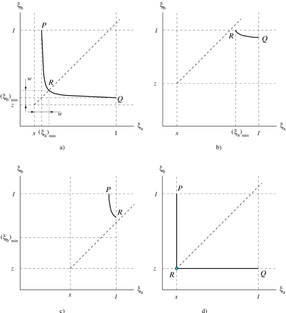
FIG. 6.: The contours of the integration over $\xi_{a}$, $\xi_{b}$ for a,b,c) the perturbative cross-section (33); d) the asymptotic and resummed cross-sections (45) and (52).

VI Numerical results

In this section, we present the results of Monte-Carlo simulations for the $z$-flow and the differential multiplicity of charged particle production,

$$\frac{1}{d\sigma_{tot}/(dxdQ^{2})}\frac{d\Sigma_{z}}{dxdQ^{2}dq_{T}}\mbox{ and }\frac{1}{d\sigma_{tot}/(dxdQ^{2})}\frac{d\sigma^{chgd}}{dxdzdQ^{2}dq_{T}}.$$

Our calculations use the parameters of the HERA electron-proton collider. The energies of the proton and electron beams are taken to be equal to 820 and 27.5 GeV, respectively.

A Energy flows

As a first application of the resummation formalism, we consider the c.m. pseudorapidity distributions of the transverse energy flows in the current region, data for which has been published in [11]. We discuss the data in seven bins of $x$ and $Q$, four of them covering the region $10\leq Q^{2}\leq 20\ \mbox{GeV}^{2}$, $3.7\cdot 10^{-4}\leq x\leq 2.3\cdot 10^{-3}$, and the other three the region $20\leq Q^{2}\leq 50\ \mbox{GeV}^{2}$, $9.3\cdot 10^{-4}\leq x\leq 4.9\cdot 10^{-3}$.

FIG. 7.: Comparison of the NLO perturbative (134) and resummed (87) expressions for the $z$-flow distribution with the existing experimental data from HERA [11]. The presented data is for $\langle x\rangle=0.0049,\ \langle Q^{2}\rangle=32.6\ \mbox{GeV}^{2}$.

FIG. 8.: Comparison of the resummed (87) $z$-flow distribution with the HERA data from [11] in 7 bins of $\langle x\rangle$ and $\langle Q\rangle$. The resummed $z$-flows were calculated using the parameterization (108) for the non-perturbative part of the Sudakov factor.

In our calculation, we use the CTEQ4M parton distribution functions [25]. The factorization and renormalization scales of the perturbative and asymptotic pieces are all set equal to $\mu=Q$. As was mentioned in Section IV, the data on transverse energy flow can be easily transformed into the $q_{T}$ distributions of the $z$-flow. In Fig. 7, we present the comparison of the existing data in one of the bins of $x$ and $Q^{2}$ ($\langle x\rangle=0.0049,\ \langle Q^{2}\rangle=32.6\ \mbox{GeV}^{2}$) with the NLO perturbative and resummed $z$-flows given in Eqs. (134) and (87), respectively. In Fig. 8 we present the comparison of the resummed $z$-flow with the data in the other bins of [11].

Figure 7 demonstrates two important aspects of the NLO $q_{T}$ distribution, namely, that the NLO exceeds the data at small $q_{T}$ and is below the data at $q_{T}\geq Q$. In fact, we find that the deficit of the NLO prediction of perturbative theory in comparison with the data at medium and large $q_{T}$ ($q_{T}\geq 5\ \mbox{GeV}$) is present in the entire region of $x$ and $Q^{2}$ that we have studied.

As we discussed in Section V, one can trust the resummed calculation only for reasonably small values of $q_{T}/Q$. For large values of $q_{T}$, the fixed-order perturbative result is more reliable. This means that the NLO resummation formalism will not give an accurate description of the data for $q_{T}\gg Q$, due to the small magnitude of the NLO perturbative $z$-flow in this region.

The excess of the data over the NLO calculation can be interpreted as a signature of other intensive hadroproduction mechanisms at c.m. pseudorapidities $\eta^{cm}\leq 2$. A discussion of the cross-sections in this pseudorapidity region is beyond the scope of our paper. However, we would like to point out that there exist several possible explanations of the data in this region, for instance, the enhancement of the cross-section due to BFKL showering [13] or resolved photon contributions [16, 18]. From the point of view of our study, it is clear that good agreement between the data and the combination of the perturbative calculation and the CSS resummation, in a wider range of $\eta^{cm}$, will be achieved when next-to-next-to-leading order contributions, like the ones contributing to (2+1) jet production [17], are taken into account.

On the other hand, Figs. 7 and 8 illustrate that the resummation formalism accurately describes the data in the region $q_{T}\leq 10\ \mbox{GeV}$. This calculation of the resummed $z$-flows (87) was done using the following parameterization for the non-perturbative Sudakov factor (90)

$$S^{NP}_{z}(b,x,Q)=g^{(1)}(b,x)+g^{(2)}(b,Q),$$ (108)

where the $Q$-dependent part $g^{(2)}(b,Q)$ is completely defined by the symmetry between semi-inclusive DIS, Drell-Yan and $e^{+}e^{-}$ hadroproduction processes (Section III),

$$g^{(2)}(b,Q)=\frac{1}{2}b^{2}\Biggl{(}0.48\log(\frac{Q}{2Q_{0}})+5.32C_{F}\log\Bigl{(}\frac{b}{b_{*}}\Bigr{)}\log\Bigl{(}\frac{C_{2}Q}{C_{1}Q_{0}}\Bigr{)}\Biggr{)}.$$ (109)

The parameterizations of the $Q$-dependent parts of the non-perturbative Sudakov factors in the Drell-Yan and $e^{+}e^{-}$ hadroproduction processes are taken from [20] and [24], respectively. In (109), the constants are $C_{1}=2e^{-\gamma},\ C_{2}=e^{-3/4},Q_{0}=1\ \mbox{GeV}$. The variable $b_{*}$ is given by (72), with $b_{max}=1\ \mbox{GeV}^{-1}$.

FIG. 9.: The comparison of the $z$-flow distributions for $\langle x\rangle=0.0049\mbox{ and }\langle Q^{2}\rangle=32.6\ \mbox{GeV}^{2}$, calculated with (solid) and without (dashed) the kinematic correction (107).

The $x$-dependent function $g^{(1)}(x,Q)$ was determined by fitting the HERA data of [11]. We found that good agreement with the data is obtained when $g^{(1)}(b,x)$ is parameterized by a linear function of $x^{-0.5}$,

$$g^{(1)}(b,x)=b^{2}\biggl{(}-2.58+\frac{0.58}{\sqrt{x}}\biggr{)},\quad\mbox{ for }x\leq 10^{-2}.$$ (110)

We should emphasize that we don’t know the exact behavior of $g^{(2)}(b,x)$ for $x\geq 10^{-2}$, where currently there is no data available. On the other hand, the term $g^{(2)}(b,x)$ in the parameterization (110) becomes negative for $x\geq 5\cdot 10^{-2}$ which makes the numerical value of the resummed $z$-flow (87) unphysical. Thus, the parameterization (110) must be used only at $x\leq 10^{-2}$.

FIG. 10.: The dependence of the resummed $z$-flow on the perturbative scale $\mu$ and the constants $C_{1},C_{2}$. The Figure corresponds to $\langle x\rangle=0.0049,\ \langle Q^{2}\rangle=32.6\ \mbox{GeV}^{2}$. The curves correspond to: $C_{1}=2e^{-\gamma}$, $C_{2}=e^{-3/4},\mu=Q$ (solid); $C_{1}=2e^{-\gamma}$, $C_{2}=e^{-3/4},\mu=2Q$ (dashed); $C_{1}=2e^{-\gamma}$, $C_{2}=e^{-3/4},\mu=0.5Q$ (dotted); $C_{1}=2e^{-\gamma}$, $C_{2}=1,\mu=Q$ (dot-dashed).

The theoretical results in Fig. 8 were obtained using the kinematic correction to the asymptotic and resummed cross-sections at non-zero $q_{T}$, which was discussed in Section V. As can be seen from Fig. 9, without this correction the agreement between the resummation calculation and the data is still good in the region $q_{T}\leq 2\ \mbox{GeV}\leq Q$, where the resummation calculation is truly applicable. The kinematic correction improves the agreement between the resummed $z$-flow and the data in the region $q_{T}\geq 2\ \mbox{GeV}$. In this region, the theoretical prediction without the kinematic correction significantly exceeds the data. As explained in Section V, this can be attributed to differences between the phase space of the perturbative and resummed pieces. In the case of the resummed cross-section the phase space may expand to much lower $x$ and $z$ than is allowed for the perturbative cross-section. Consequently, the large magnitude of PDFs and FFs at small $x$ and $z$ may spoil the cancellation between the resummed and asymptotic piece at large $q_{T}$. This difference can be corrected by redefinition (107) of the variables $x$ and $z$ in the resummed and asymptotic pieces.

FIG. 11.: Dependence of the resummed $z$-flow on $Q_{0}$ and $b_{max}$. The curves correspond to $Q_{0}=1\ \mbox{GeV}$, $b_{max}=1\ \mbox{GeV}^{-1}$ (thick solid); $Q_{0}=1\ \mbox{GeV}$, $b_{max}=0.5\ \mbox{GeV}^{-1}$ (dashed); $Q_{0}=1\ \mbox{GeV}$, $b_{max}=2\ \mbox{GeV}^{-1}$ (dotted); $Q_{0}=0.5\ \mbox{GeV}$, $b_{max}=1\ \mbox{GeV}^{-1}$ (thin solid); $Q_{0}=2\ \mbox{GeV}$, $b_{max}=1\ \mbox{GeV}^{-1}$ (dot-dashed). The graph corresponds to $\langle x\rangle=0.0049,\ \langle Q^{2}\rangle=32.6\ \mbox{GeV}^{2}$.

One of the advantages of the resummed cross-sections is that, by their construction, they are less dependent on the choice of the renormalization and factorization scales of the problem, and on the end points $C_{1}/b$ and $C_{2}Q$ in the integral of the perturbative Sudakov factor (55). The reason is that the scale variations in the perturbative part of (87) are compensated by the variation of the term $g^{(2)}(b,Q)$ in the nonperturbative Sudakov factor (108).

In Fig. 10 we show the resummed $z$-flow for different choices of perturbative renormalization and factorization scale $\mu$, varying between $0.5Q$ and $2Q$, and for a different choice of the constants $C_{1}$ and $C_{2}$ (the “canonical choice” $C_{1}=2e^{-\gamma},\ C_{2}=1$). As expected, the resummed cross-section shows little variation with the changes of $\mu,\ C_{1},\ C_{2}$.

We have also checked the stability of the resummed $z$-flow under variation of the momentum transfer scale $Q_{0}$ in the logarithm of $g^{(2)}(b,Q)$, and under variation of the parameter $b_{max}$ separating the perturbative and nonperturbative dynamics in (87). Fig. 11 shows the $z$-flows for variations of $Q_{0}$ and $b_{max}$ by factors of $1/2$ and $2$. As can be seen in Fig. 11, the variation of the resummed $z$-flow is small. The stability of the resummed $z$-flow under the variation of $b_{max},Q_{0},C_{1},C_{2}$ indicates that the choice of these parameters has less influence on the shape of the resummed cross-section than the free parameters in $g^{(1)}(b,x)$. It also illustrates the fact that the existing HERA data is relatively insensitive to the parameterization of the $Q$-dependent function $g^{(2)}(b,Q)$, which can be studied in a more detailed fashion once the data in a larger range of $Q$ become available.

Finally, in Fig. 12 we replot the results of our calculation presented in Fig. 8 as the c.m. pseudorapidity distributions of the transverse energy flow $\langle E_{T}\rangle$. This quantity is obtained by the transformation (83). The small-$q_{T}$ region, where the resummation formalism is valid, corresponds to large pseudorapidities. In this region, the agreement between our calculation and the data is good. At smaller pseudorapidities (larger $q_{T}$), one sees the above-mentioned excess of the data over the perturbative NLO calculation. In the $\langle E_{T}\rangle$ vs. $\eta_{cm}$ plot, this excess is magnified because of the factor $q_{T}^{2}$ in the transformation (83).

FIG. 12.: The $\gamma^{*}p$ c.m. pseudorapidity distributions of the transverse energy flow in the current region. The data are from [11].

FIG. 13.: The charged particle multiplicity at $\langle x\rangle=0.0044$, $\langle Q^{2}\rangle=35\ \mbox{GeV}^{2}$.

B Multiplicity of charged particle production

The H1 and ZEUS collaborations recently published the pseudorapidity distributions of charged particle multiplicity at small values of $x$ and $Q^{2}$ [8]. The data presented was organized in the same bins of $x$ and $Q^{2}$ as those used in the H1 analysis of the transverse energy flow [11]. Also, the experiment E665 at Fermilab has provided extensive data on charged particle multiplicity covering the region of larger $x$ [10]. However, a comparison of these data with our calculation, analogous to the one described in the previous subsection, is complicated by several obstacles.

In comparison to energy flows, charged particle multiplicity depends on the additional variable $z$ which controls the fragmentation of a final-state parton into the observed hadrons. Therefore the pQCD hadroproduction cross-sections depend on parton fragmentation functions $D(\xi_{b},\mu)$, which at present are known well only in the region $0.1\leq\xi_{b}\leq 0.8$ [26].

The non-perturbative Sudakov factor (90) for particle multiplicity can depend on $z$. Furthermore, in principle the non-perturbative Sudakov factor can be different for different types of initial and final states (see the discussion of Eq. (75) above). As a first approximation, in the analysis below we will ignore this difference.

On the other hand, in the existing data on charged particle pseudorapidity or transverse momentum distributions [8, 10] the dependence on the final-state fragmentation variable is not separated from the other variables. Therefore more complicated fitting of the data is necessary to disentangle the $q_{T}$ and $z$ dependences.

More importantly, our calculation was made under the assumption that all the participating particles, including the final-state hadrons, are massless. Because of this assumption, the production of soft final-state hadrons, with $z=0$ is allowed. This contradicts the situation of the experiments at HERA and Fermilab, in which there is a non-zero minimal value of $z$ determined by the finite mass of the observed hadron. It follows from the definition (5) of $z$ and the formulas (24, 25) for the initial and final hadron momenta in the $\gamma^{*}p$ c.m. frame, that

$$z=\frac{p_{B+}^{cm}}{W}\geq\frac{m_{B}}{W},$$ (111)

where

$$p_{B+}^{cm}=E_{B}^{cm}+p_{Bz}^{cm}\mbox{ and }W^{2}=Q^{2}\Bigl{(}\frac{1}{x}-1\Bigr{)}.$$

Using (111), one can show that the multiplicity distributions presented in [8] receive contributions from charged pions with $z\approx 10^{-3}$ or lower. This means that for the experimental cuts used in the H1 analysis, the multiplicity receives significant contribution from the region $z\leq 0.1$ where the fragmentation functions are poorly known, and mass effects are important.

In Fig. 13 we present the resummed multiplicity in the region $z\geq 0.1$, where the uncertainties in our knowledge of the fragmentation functions and the mass effects are minimal. The results in Fig. 13 are given for $x=0.0044,\ Q^{2}=35\ \mbox{GeV}^{2}$ and various bins of $z$. In the calculation, we used the CTEQ4M PDFs [25] and the fragmentation functions from [26]. We show the prediction using the $z$-independent non-perturbative Sudakov factor (108) obtained from the study of the energy flows. We also assume that the charged particle production rate is dominated by fragmentation of partons into charged pions, kaons and protons, and that the non-perturbative Sudakov factors for these types of particles are the same. In spite of many assumptions that go into this calculation, it will be interesting to compare it with the experimental data.

VII Conclusions

In this paper, we have presented a formalism for all-order resummation of large logarithms arising in hadroproduction in the current region of deep-inelastic scattering, i.e. for large pseudorapidity of the final-state hadrons in the photon-proton cm. frame. We found that the formalism describes well the behavior of the transverse energy flows measured at HERA [11] in the region of large hadronic c.m. pseudorapidity $\eta\geq 3.0$. At smaller pseudorapidities, we found a deficit of the NLO rate compared to the existing data. Evidently, this is a signature of the importance of the NNLO corrections, which were not studied in this paper.

The formalism presented here can also be directly applied to the study of hadron multiplicities. In this case, however, additional care is required in treating the final-state fragmentation of partons and the effects of the mass of the final-state hadron. In view of this, reanalysis of charged particle production multiplicity measured by H1, ZEUS and Fermilab-E665, with the goal to separate the $z$ and $q_{T}$ dependence, will be very useful to study the properties of the non-perturbative part of the Sudakov factor, and to improve the applicability of the perturbative calculation in the current region.

Appendix A. Transformation from the hadron frame to the HERA lab frame

In this Appendix, we summarize the relationships between the relativistic invariants used in this paper, the hadron frame variables, and the particle momenta in the HERA lab frame.

The definition of the HERA lab frame is that the proton ($A$) moves in the $+z$ direction, with energy $E_{A}$, and the incoming lepton moves in the $-z$ direction with energy $E$. The momenta of the incident particles are

$$p_{A}^{\mu}=(E_{A},0,0,E_{A}),$$ (112)

$$l^{\mu}=(E,0,0,-E)~{}.$$ (113)

The outgoing lepton has energy $E^{\prime}$ and scattering angle $\theta$ relative to the $-z$ direction. We define the $x$-axis of the HERA frame such that the outgoing lepton is in the $xz$-plane; that is,

$$l^{\prime\mu}_{l}=(E^{\prime},-E^{\prime}\sin\theta,0,-E^{\prime}\cos\theta)~{}.$$ (114)

The observed hadron ($B$) has energy $E_{B}$ and scattering angle $\theta_{B}$ with respect to the $+z$ direction, and azimuthal angle $\phi_{B}$; thus its momentum is

$${p_{B}^{\mu}}_{l}=(E_{B},E_{B}\sin\theta_{B}\cos\phi_{B},E_{B}\sin\theta_{B}\sin\phi_{B},E_{B}\cos\theta_{B})~{}.$$ (115)

The scalars $x$ and $Q^{2}$ are completely determined by measuring the energy and the scattering angle of the outgoing lepton,

$$Q^{2}=2EE^{\prime}(1-\cos\theta),$$ (116)

$$x=\frac{EE^{\prime}(1-\cos\theta)}{E_{A}\left[2E-E^{\prime}(1+\cos\theta)\right]}~{}.$$ (117)

The scalars $z$ and $q_{T}^{2}$ depend on the outgoing hadron and lepton as

$$z=\frac{\beta E_{B}(1-\cos\theta_{B})}{Q},$$ (118)

$$q_{T}^{2}=\frac{2\,{Q^{2}}\,\left(1-\left(y-1\right)\,{{\beta}^{2}}\right)}{{{\beta}^{2}(1-\cos\theta_{B})}}\Biggl{[}\sin^{2}\frac{\theta_{B}-\theta_{*}}{2}+\sin\theta_{B}\sin\theta_{*}\sin^{2}\frac{\phi_{B}}{2}\Biggr{]},$$ (119)

where

$$y=\frac{Q^{2}}{xS_{eA}},\ \beta=\frac{2xE_{A}}{Q},\ cot\frac{\theta_{*}}{2}=\beta\sqrt{1-y}.$$ (120)

The angle $\phi$ and the boost parameter $\psi$, which are used for the angular decomposition of the cross-sections in the hadron Breit frame, can be found as

$$\cos\phi=\frac{Q}{2\,{\sqrt{1-y}}\,{q_{T}}}\,\left[1-y-\frac{\cot^{2}(\theta_{B}/2)}{\beta^{2}}+\frac{q_{T}^{2}}{Q^{2}}\right],$$ (121)

$$\cosh\psi=\frac{2}{y}-1.$$ (122)

Appendix B. The perturbative cross-section and $z$-flow distribution

In this Appendix, we collect the formulas for the NLO parton level cross-sections $d\hat{\sigma}_{ba}/(d\hat{x}d\hat{z}dQ^{2}dq_{T}^{2}d\phi)$.

According to (33), the hadron level cross-section $d\sigma_{BA}/(dxdzdQ^{2}dq_{T}^{2}d\phi)$ is related to the parton cross-sections $d\sigma_{ba}/(d\hat{x}d\hat{z}dQ^{2}dq_{T}^{2}d\phi)$ as

$$\frac{d\sigma_{BA}}{dxdzdQ^{2}dq_{T}^{2}d\phi}=\sum_{a,b}\int_{z}^{1}\frac{d\xi_{b}}{\xi_{b}}D_{B/b}(\xi_{b})\int_{x}^{1}\frac{d\xi_{a}}{\xi_{a}}F_{a/A}(\xi_{a})\frac{d\hat{\sigma_{ba}}}{d\hat{x}d\hat{z}dQ^{2}dq_{T}^{2}d\phi}.$$

At non-zero $q_{T}$, the parton cross-section receives the contribution from the real emission diagrams (Fig. 4e-f); it can be expressed as

$$\frac{d\hat{\sigma}_{ba}}{d\hat{x}d\hat{z}dQ^{2}dq_{T}^{2}d\phi}=$$ (123)

$$\frac{\sigma_{0}F_{l}}{4\pi S_{eA}Q^{2}}\frac{\alpha_{s}}{\pi}\delta\Biggl{[}\frac{q_{T}^{2}}{Q^{2}}-\Bigl{(}\frac{1}{\hat{x}}-1\Bigr{)}\Bigl{(}\frac{1}{\hat{z}}-1\Bigr{)}\Biggr{]}\sum_{j}e^{2}_{j}\sum_{\alpha=1}^{4}f^{(\alpha)}_{ba}(\hat{x},\hat{z},Q^{2},q_{T}^{2})A_{\alpha}(\psi,\phi),$$ (124)

with the same notations as in Section III. In this formula,

$$\sum_{\alpha=1}^{4}f^{(\alpha)}_{jk}(\hat{x},\hat{z},Q^{2},q_{T}^{2})A_{\alpha}(\psi,\phi)=2\delta_{jk}C_{F}\hat{x}\hat{z}\Biggl{\{}\Bigl{[}\frac{1}{q_{T}^{2}}\biggl{(}\frac{Q^{4}}{\hat{x}^{2}\hat{z}^{2}}+(Q^{2}-q_{T}^{2})^{2}\biggr{)}+6Q^{2}\Bigr{]}A_{1}$$ (125)

$$+ 2Q^{2}(2A_{2}+A_{4})+2\frac{Q}{q_{T}}(Q^{2}+q_{T}^{2})A_{3}\Biggr{\}};$$ (126)

$$\sum_{\alpha=1}^{4}f^{(\alpha)}_{jg}(\hat{x},\hat{z},Q^{2},q_{T}^{2})A_{\alpha}(\psi,\phi)=$$ (128)

$$\hat{x}(1-\hat{x})\Biggl{\{}\Bigl{[}\frac{Q^{4}}{q_{T}^{2}}\biggl{(}\frac{1}{\hat{x}^{2}\hat{z}^{2}}-\frac{2}{\hat{x}\hat{z}}+2\biggr{)}+2Q^{2}(5-\frac{1}{\hat{x}}-\frac{1}{\hat{z}})\Bigr{]}A_{1}$$

$$+ 4Q^{2}(2A_{2}+A_{4})+2\frac{Q}{q_{T}}(2(Q^{2}+q_{T}^{2})-\frac{Q^{2}}{\hat{x}\hat{z}})A_{3}\Biggr{\}};$$ (129)

$$\sum_{\alpha=1}^{4}f^{(\alpha)}_{gj}(\hat{x},\hat{z},Q^{2},q_{T}^{2})A_{\alpha}(\psi,\phi)=$$ (131)

$$2C_{F}\hat{x}(1-\hat{z})\Biggl{\{}\Bigl{[}\frac{1}{\tilde{q}_{T}^{2}}\biggl{(}\frac{Q^{4}}{\hat{x}^{2}(1-\hat{z})^{2}}+(Q^{2}-\tilde{q}_{T}^{2})^{2}\biggr{)}+6Q^{2}\Bigr{]}A_{1}$$

$$+ 2Q^{2}(2A_{2}+A_{4})+2\frac{Q}{\tilde{q}_{T}}(Q^{2}+\tilde{q}_{T}^{2})A_{3}\Biggr{\}}.$$ (132)

In (132),

$$\tilde{q}_{T}=\frac{\hat{z}q_{T}}{1-\hat{z}}.$$ (133)

The index $j$ corresponds to a quark (antiquark) of a type $j$, the index $g$ corresponds to a gluon.

From (33), it is possible to derive the perturbative $z$-flow distribution,

$$\frac{d\Sigma_{z}}{dxdQ^{2}dq_{T}^{2}d\phi}\equiv\sum_{B}\int_{z_{min}}^{1}zdz\frac{d\sigma_{BA}}{dxdzdQ^{2}dq_{T}^{2}d\phi}=$$

$$\frac{\sigma_{0}F_{l}}{4\pi S_{eA}Q^{2}}\frac{\alpha_{s}}{\pi}\sum_{a,b}\sum_{j}e^{2}_{j}\int_{x}^{1}\frac{d\xi_{a}}{\xi_{a}-x}F_{a/A}(\xi_{a})\hat{z}^{3}\hat{x}\sum_{\alpha=1}^{4}f^{(\alpha)}_{ba}(\hat{x},\hat{z},Q^{2},q_{T}^{2})A_{\alpha}(\psi,\phi).$$ (134)

It depends on the same functions $f_{ba}(\hat{x},\hat{z},Q^{2},q_{T}^{2})$, with the parton variable $\hat{z}$ determined by the $\delta$-function in (124),

$$\hat{z}=\frac{1-\hat{x}}{(q_{T}^{2}/Q^{2}-1)\hat{x}+1}.$$ (135)

REFERENCES

- [1] Y. I. Dokshitser, D. I. D’yakonov, S. I. Troyan, Phys. Lett. 79B, 269 (1978).
- [2] G. Parisi, R. Petronzio, Nucl. Phys. B154, 427 (1979)
- [3] G. Altarelli, R. K. Ellis, M. Greco, G. Martinelli, Nucl. Phys. B246, 12 (1984).
- [4] J. Collins, D. Soper, Nucl. Phys. B193, 381 (1981); Nucl. Phys. B197, 446 (1982); Acta Phys. Polon. B16, 1047 (1985).
- [5] J. Collins, D. Soper, G. Sterman, Nucl. Phys. B250, 199 (1985).
- [6] C. Balazs, E. L. Berger, S. Mrenna, C.-P. Yuan, Phys.Rev. D57, 6934 (1998).
-
[7]
I. Hinchliffe, S. F. Novaes, Phys. Rev. D38, 3475 (1988);
R. P. Kaufmann, Phys. Rev. D44 (1991) 1415;
C.-P. Yuan, Phys. Lett. B283, 395 (1992). - [8] H1 Coll., Nucl. Phys. B485, 3 (1997); ZEUS Coll., Z. Phys. C70, 1 (1996).
-
[9]
H1 Coll., Z. Phys. C63, 377 (1994); C70,
609 (1996); C72, 573 (1996); Phys. Lett. B328, 176 (1994);
ZEUS Coll., Z. Phys. C70, 1, (1996). - [10] E665 Coll., Z. Phys. C76 , 441 (1997).
- [11] H1 Coll., Phys. Lett. B356, 118 (1995).
- [12] D. Graudenz, Phys. Lett. B406, 178 (1997); Fortsch.Phys. 45, 629 (1997).
-
[13]
E.A. Kuraev, L.N. Lipatov, V.S. Fadin, Sov. Phys. JETP
45, 199, (1977);
Ya. Ya. Balitsky, L. N. Lipatov, Sov. J. Nucl. Phys. 28, 822,1978. - [14] R. Meng, F. Olness, D. Soper, Nucl. Phys. B371, 79 (1992).
- [15] R. Meng, F. Olness, D. Soper, Phys.Rev. D54, 1919 (1996).
-
[16]
M. Klasen, T. Kleinwort, G. Kramer, Eur.Phys.J., C1, 1 (1998);
B. Potter, preprint DESY-97-138; Comp. Phys. Comm., 119, 45 (1999);
G. Kramer, B. Potter, Eur. Phys. J. C5, 665 (1998). - [17] S. Catani, M.H. Seymour, Phys. Lett. B378, 287 (1996); Nucl. Phys. B485, 291, (1997); D. Graudenz, hep-ph/9708362.
- [18] H. Jung, L. Jonsson, H. Kuster, preprint DESY-98-051, hep-ph/9805396.
- [19] T. P. Cheng, Wu-Ki Tung, Phys. Rev. D3, 733 (1971); C.S. Lam, Wu-Ki Tung, Phys. Rev., D18, 2447 (1978); F. Olness, Wu-Ki Tung, Phys. Rev. D35, 833 (1987).
- [20] C.T.H. Davies, B.R. Webber, W.J. Stirling, Nucl. Phys. B256, 413 (1985).
- [21] G.A. Ladinsky, C.-P. Yuan, Phys. Rev. D50, 4239 (1994).
- [22] C. Balazs, C.-P. Yuan, Phys. Rev. D56, 5558, (1997).
- [23] F. Landry, R. Brock, G. Ladinsky, and C.-P. Yuan, preprint CTEQ-904, hep-ph/9905391.
- [24] J. Collins, D. Soper, Nucl. Phys. B284, 253 (1987).
- [25] H.-L. Lai et al., CTEQ Coll., Phys. Rev. D55, 1280 (1997).
- [26] J. Binnewies, B. A. Kniehl, G. Kramer, Phys. Rev. D52, 4947 (1995).