End-point of the Electroweak Phase Transition using the auxiliary mass method

Abstract

We study the end-point of the Electroweak phase transition using the auxiliary mass method. The end point is $m_{H}\sim 40$ (GeV) in the case $m_{t}=0$ (GeV) and strongly depends on the top quark mass. A first order phase transition disappears at $m_{t}\sim 160$ (GeV). The renormalization effect of the top quark is significant.

The Electroweak phase transition is one of the most important phase transitions at the early universe since it may account for the baryon number of the present universe[1]. This phase transition was first investigated using the perturbation theory of the finite temperature field theory and predicts the first order phase transition from an effective potential[2, 3]. The perturbation theory, however, has difficulty due to an infrared divergence caused by light Bosons and cannot give reliable results in the case where the Higgs Boson mass $m_{H}$, is comparable to or greater than the Weak Boson mass. Lattice Monte Carlo simulations, therefore, become the most powerful method and are still used to investigate details of the phase transition[4, 5, 6, 7, 8]. According to these results, the Electroweak phase transition is of the first order if $m_{H}$ is less than an end-point $m_{H,c}\sim 70$ (GeV). It turns to be of the second order just on the end-point. Beyond the end-point, we have no phase transition, which means any observable quantities do not have discontinuities. As far as we know, three other non-perturbative methods predict the existence of the end-point[9, 10, 11]. The end-point is determined below 100 GeV by these three methods.

The auxiliary-mass method is a new method to avoid the infrared divergence at a finite temperature T[12, 13, 14, 15]. This method is based on a simple idea as follows. We first add a large auxiliary mass to light Bosons, which cause the infrared divergence, and calculate an effective potential at the finite temperature. Due to the auxiliary mass, the effective potential is reliable at any temperature. We next extrapolate this effective potential to the true mass by integrating an evolution equation, which we show later. We applied this method to the $Z_{2}$-invariant scalar model and the $O(N)$-invariant scalar model, and obtained satisfactory results[13, 14, 15].

We apply the method to the Standard Model and investigate the Electroweak phase transition in the present paper. We add an auxiliary mass $M\gtrsim T$ only to the Higgs Boson, which becomes very light owing to a cancellation between its negative tree mass and positive thermal mass for small field expectation values around the critical temperature. We notice that the infrared divergence from the Higgs Boson is always serious if the phase transition is of the second order or of the weakly first order[3]. In the standard model, transverse modes of the gauge fields also have small masses at small field expectation values since they do not have the thermal mass at one loop order. It is however, expected that they do have a thermal mass ($\sim g^{2}T$) at the two loop order[7, 9, 16]. Here, $g$ is a gauge coupling constant. If so, the loop expansion parameter[3] is $\frac{g^{2}T}{M_{G}}\lesssim 1$, even if the field expectation value is zero. Here, $M_{G}$ is the mass of the gauge Boson, which is a sum of a zero-temperature mass and a thermal mass. We assume that this actually occurs and the infrared divergence from the gauge Bosons is not serious. Since this small thermal mass for the transverse modes will bring only a slight change to a one-loop effective potential, we use the one-loop effective potential without this small mass for the transverse modes.

An effective potential is then calculated as follows in the Landau gauge[2, 3],

$$V(M^{2}) = \frac{M^{2}}{2}\phi^{2}+\frac{\lambda}{4!}\phi^{4}+f_{BT}(m_{H}^{2}(\phi))+3f_{BT}(m_{NG}^{2}(\phi))$$ (7)

$$+4f_{BT}(M_{W}^{2}(\phi))+4f_{G0}(M_{W}^{2}(\phi))$$

$$+2f_{BT}(M_{WL}^{2}(\phi))+2f_{G0}(M_{WL}^{2}(\phi))$$

$$+2f_{BT}(M_{Z}^{2}(\phi))+2f_{G0}(M_{Z}^{2}(\phi))$$

$$+f_{BT}(M_{ZL}^{2}(\phi))+f_{G0}(M_{ZL}^{2}(\phi))$$

$$+f_{BT}(M_{\gamma L}^{2}(\phi))+f_{G0}(M_{\gamma L}^{2}(\phi))$$

$$+12f_{FT}(m_{t}^{2}(\phi))+12f_{F0}(m_{t}^{2}(\phi))$$

here,

$$m_{H}^{2}(\phi) = M^{2}+\frac{\lambda}{2}\phi^{2},\ m_{NG}^{2}(\phi)=M^{2}+\frac{\lambda}{6}\phi^{2},$$ (8)

$$M_{W}^{2}(\phi) = \frac{g_{2}^{2}\phi^{2}}{4},\ M_{WL}^{2}(\phi)=\frac{g_{2}^{2}\phi^{2}}{4}+\frac{11g_{2}^{2}T^{2}}{6},$$ (9)

$$M_{Z}^{2}(\phi) = \frac{(g_{2}^{2}+g_{1}^{2})\phi^{2}}{4},\ m_{t}(\phi)=\frac{g_{Y}^{2}\phi^{2}}{2}$$ (10)

$$\left(\begin{array}[]{cc}M_{ZL}^{2}&0\\ 0&M_{\gamma L}^{2}\end{array}\right) = {\bf T^{\dagger}}\left(\begin{array}[]{cc}\frac{g_{2}^{2}\phi^{2}}{4}+\frac{11g_{2}^{2}T^{2}}{6}&-\frac{g_{1}g_{2}\phi^{2}}{4}\\ -\frac{g_{1}g_{2}\phi^{2}}{4}&\frac{g_{1}^{2}\phi^{2}}{4}+\frac{11g_{2}^{2}T^{2}}{6}\end{array}\right){\bf T}$$ (15)

$$f_{BT}(m^{2}) = \frac{T}{2\pi^{2}}\int_{0}^{\infty}dk\ k^{2}\log{\{1-\exp{(-\frac{\sqrt{k^{2}+m^{2}}}{T})}\}}$$ (16)

$$f_{FT}(m^{2}) = \frac{T}{2\pi^{2}}\int_{0}^{\infty}dk\ k^{2}\log{\{1+\exp{(-\frac{\sqrt{k^{2}+m^{2}}}{T})}\}}$$ (17)

$$f_{G0}(m^{2}) = \frac{m^{4}}{64\pi^{2}}\{\log{(\frac{m^{2}}{\bar{\mu}^{2}})}-\frac{5}{6}\}$$ (18)

$$f_{F0}(m^{2}) = -\frac{m^{4}}{64\pi^{2}}\{\log{(\frac{m^{2}}{\bar{\mu}^{2}})}-\frac{3}{2}\}.$$ (19)

In the above equations, $\lambda$, $g_{2}$, $g_{1}$ and $g_{Y}$ are coupling constants for the Higgs Boson, SU(2) gauge field, U(1) gauge field and top Yukawa respectively. The matrix ${\bf T}$ is orthogonal and diagonalizes the mass matrix for the Z Boson and photon at finite temperature. We renormalized the effective potential using the $\overline{MS}$ scheme with a renormalization scale $\bar{\mu}$. A zero-temperature contribution from the Higgs Boson is neglected since it is small in the mass region we consider. The ring diagrams are added only to the Weak Bosons and the Z-Boson since the Higgs Bosons have auxiliary large mass and do not need the resummation. We then extrapolate this effective potential at the auxiliary mass squared $M^{2}$ to that of the true mass squared $-\nu^{2}$ using an evolution equation. Since we add the auxiliary mass only to the Higgs Boson, the evolution equation is same as that for O(4)-invariant scalar model, which was constructed in [15],

$$\frac{\partial V}{\partial m^{2}} = \frac{1}{2}\bar{\phi}^{2}+\frac{1}{4\pi^{2}}\int^{\infty}_{0}dk\frac{k^{2}}{\sqrt{k^{2}+\frac{\partial^{2}V}{\partial\bar{\phi}^{2}}}}\frac{1}{e^{\frac{1}{T}\sqrt{k^{2}+\frac{\partial^{2}V}{\partial\bar{\phi}^{2}}}}-1}$$ (21)

$$+\frac{3}{4\pi^{2}}\int^{\infty}_{0}dk\frac{k^{2}}{\sqrt{k^{2}+\frac{1}{\bar{\phi}}\frac{\partial V}{\partial\bar{\phi}}}}\frac{1}{e^{\frac{1}{T}\sqrt{k^{2}+\frac{1}{\bar{\phi}}\frac{\partial V}{\partial\bar{\phi}}}}-1}.$$

A non-perturbative effective potential free from the infrared divergence can be obtained by solving the evolution equation (21) with an initial condition Eq.(7) numerically.

Before showing our numerical results, we relate the parameters $\nu^{2}$, $\lambda$, $g_{2}$, $g_{1}$ and $g_{Y}$ to physical quantities at the zero-temperature[3],

$$\lambda = \frac{3m_{H0}^{2}}{\phi_{0}^{2}}-\frac{3}{32\pi^{2}}\left[\frac{3}{2}g_{2}^{4}\left\{\log{\left(\frac{M_{W0}^{2}}{\bar{\mu}^{2}}\right)+\frac{2}{3}}\right\}\right.$$ (24)

$$+\frac{3}{4}\left(g_{1}^{2}+g_{2}^{2}\right)^{2}\left\{\log{\left(\frac{M_{Z0}^{2}}{\bar{\mu}^{2}}\right)}+\frac{2}{3}\right\}$$

$$-\left.12g_{Y}^{2}\log{\left(\frac{m_{t0}^{2}}{\bar{\mu}^{2}}\right)}\right]$$

$$\nu^{2} = \frac{m_{H0}^{2}}{2}-\frac{\phi_{0}^{2}}{64\pi^{2}}\left\{\frac{3}{2}g_{2}^{4}+\frac{3}{4}(g_{1}^{2}+g_{2}^{2})^{2}-12g_{Y}^{4}\right\}$$ (25)

$$M_{W0}^{2} = \frac{g_{2}^{2}\phi_{0}^{2}}{4},M_{Z0}^{2}=\frac{(g_{2}^{2}+g_{1}^{2})\phi_{0}^{2}}{4},$$ (26)

$$m_{t0}^{2} = \frac{g_{Y}^{2}\phi_{0}^{2}}{2},\phi_{0}=246\ {\rm(GeV)}$$ (27)

Radiative corrections at the one-loop order are included in the equations for $\nu^{2}$ and $\lambda$ since they are large, especially in the case where the Higgs Boson mass is small. The effective potential Eq.(7) does not depend on $\bar{\mu}$ using $\lambda$ in Eq.(24) in this order. We fix the masses of the Weak Bosons and the Z-Boson as $M_{W0}=80$ (GeV) and $M_{Z0}=92$ (GeV) below.

We first investigate a $SU(2)\times U(1)$ gauge plus Higgs theory, corresponding to the case $m_{t}=0$. We show results obtained by setting $M=T$ since similar results were obtained by setting $M=\frac{T}{2}$ and $M=2T$ as in the case of [13]. This is quite natural since the ristriction on $M$ is $M\gtrsim T$. The effective potentials at the critical temperature are shown in Fig.1 for $m_{H}=$15, 30, 45 (GeV), respectively. The first order phase transition becomes weaker for smaller values of the Higgs mass and disappears finally. They are compared to effective potentials obtained by the ring resumed perturbation theory at the one-loop order without the high temperature expansion in Fig.2. We find clearly that they are similar for smaller values of $m_{H}$ and different for larger values of $m_{H}$. This is consistent with the fact that the ring resumed perturbation theory is reliable only for smaller values of the Higgs mass $m_{H}\ll M_{W}$[3]. We plot a ratio of the critical field expectation values to the critical temperature, $\phi_{c}/T_{c}$, as a function of $m_{H}$ in Fig.3. This quantity indicates the strength of the first order phase transition and important in estimating the sphaleron rate, which plays a very important role in the Electroweak Baryogenesis[17, 18]. The end-point is determined as $m_{H,c}=38$ (GeV) from Fig.3. This figure also shows that the results obtained by the auxiliary mass method and the perturbation theory is similar for smaller values of $m_{H}$ and different for larger values, $m_{H}\gtrsim 30$ (GeV).

\begin{picture}(14.0,6.0)\centerline{\hbox{ \epsfbox{jcom.EPSF} }} \end{picture}

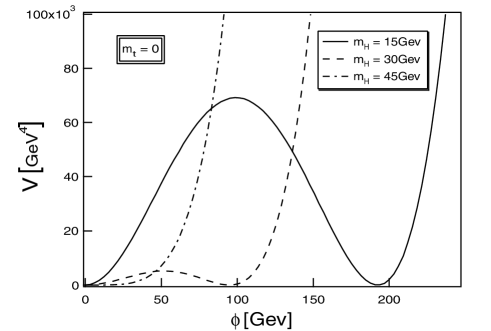
FIG. 1.: The effective potentials at the critical temperature for $m_{H}=$15, 30, 45 (GeV). The first order phase transition becomes weaker for smaller values of the Higgs mass and disappears finally.

\begin{picture}(10.0,12.0)\centerline{\hbox{ \epsfbox{jpcom.EPSF} }} \end{picture}

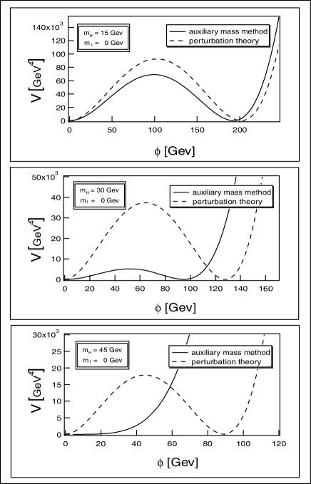
FIG. 2.: The effective potentials at the critical temperature obtained by the auxiliary mass method and the perturbation theory for $m_{H}=$15, 30, 45 (GeV). They are similar for smaller values of $m_{H}$ and different for larger values of $m_{H}$.

\begin{picture}(10.0,6.0)\centerline{\hbox{ \epsfbox{sp.EPSF} }} \end{picture}

FIG. 3.: The ratio of the critical field expectation values to the critical temperature, $\phi_{c}/T_{c}$. The results obtained by auxiliary mass method and the perturbation theory are similar for smaller values of $m_{H}$ and different for larger values, $m_{H}\gtrsim 30$ (GeV.

We next investigate more realistic cases in which the top quark mass is finite. The same ratios are shown in Fig.4 for various values of $m_{t}$. This figure shows that the strengths of the first order phase transition are almost same for $m_{t}\lesssim 100$ (GeV) and become weaker for $m_{t}\gtrsim 100$ (GeV) rapidly. The end-points are then shown in Fig.5 as a function of $m_{t}$. The graph labeled “1-loop” is obtained using Eq.(7) and Eq.(24), which take into account the zero-temperature radiative corrections from the top quark and gauge fields. The contribution from the top quark is much larger than that of the gauge fields. On the other hand, the graph labeled as “tree” is obtained without the zero-temperature radiative correction, omitting the contributions from $f_{G0}$ and $f_{F0}$ from Eq.(7) and leaving only the first terms of Eq.(24) for $\lambda$ and $\nu^{2}$. They are not much different for smaller values of the top quark mass, $m_{t}\lesssim 100$ (GeV). Their behavior, however, differs drastically for larger values of the top quark mass, $m_{t}\gtrsim 100$ (GeV). Surprisingly, the end-point vanishes for $m_{t}\gtrsim 160$ (GeV) in the “1-loop” results though it increases in the “tree” results. These results tell us that fermionic degrees of freedom play significant roles in the phase transition through the renormalization effects at the zero-temperature. We also conclude that there are no the first order phase transitions for $m_{t}=175$ (GeV), no matter how small the Higgs Boson mass.

\begin{picture}(10.0,6.0)\centerline{\hbox{ \epsfbox{sp2.EPSF} }} \end{picture}

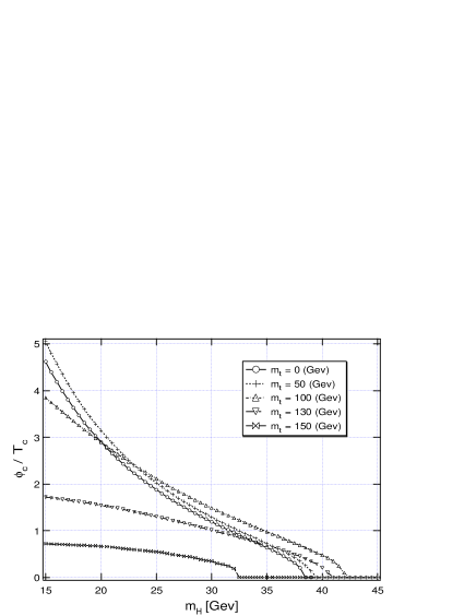
FIG. 4.: The ratio of the critical field expectation values to the critical temperature, $\phi_{c}/T_{c}$. The results obtained by the auxiliary mass method and the perturbation theory are similar for smaller values of $m_{H}$ and different for larger values, $m_{H}\gtrsim 30$ (GeV).

\begin{picture}(10.0,6.0)\centerline{\hbox{ \epsfbox{end.EPSF} }} \end{picture}

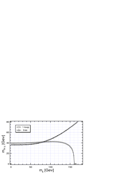
FIG. 5.: The end-points as a function of $m_{t}$. The graphs labeled as “1-loop” and “tree” are obtained with and without the zero-temperature radiative corrections from the top quark and gauge fields, respectively. The end-point vanishes for $m_{t}\gtrsim 160$ (GeV) in the “1-loop” result.

In the present paper, we have calculated the effective potentials of the standard model using the auxiliary mass method at a finite temperature. We first investigated a $SU(2)\times U(1)$ gauge plus Higgs theory, corresponding to the case $m_{t}=0$. The phase transition was of the first order and similar to the results obtained by the perturbation theory for smaller $m_{H}\sim 15$ (GeV). The phase transition became weaker for larger $M_{H}\sim 30$ (GeV) and finally disappeared in contrast to the results from perturbation theory. We found that the end-point is at $m_{H,c}=38$ (GeV) in this case. This is consistent with the results of the Lattice Monte Carlo simulation [5, 6, 7, 8] and the other non-perturbative methods[9, 10, 11] qualitatively. The value of the end-point, however, was smaller than those by these methods. This may be caused by the approximations, used to construct the evolution equation (21), or used in the other papers. The two loop effect from the gauge fields may shift our results due to slow convergence of the perturbation theory. We next investigated the more realistic case in which the top quark mass is finite. We found that the end-point was strongly dependent on $m_{t}$ and disappeared for $m_{t}\gtrsim 160$ (GeV). The renormalization effects from the top quark were significant. Lattice Monte Carlo simulations, however, do not follow this behavior[4]. We think of two possible reasons:(1)Since our results differ from that of the Lattice Monte Carlo simulation by factors of 2 in a $SU(2)\times U(1)$ gauge plus Higgs theory quantitatively, the similar behavior may be found at a larger top quark mass in the Lattice Monte Carlo simulation.(2)Since the one-loop correction to the effective potential at the zero-temperature is significant, the 3D effective theory, which has no Fermionic degrees of freedom, may not reflect the effect appropriately.

Finally, the strongly first order phase transition necessary for the Electroweak Baryogenesis was not found in the Standard Model. We will apply this method to extensions of the Standard Model.

The authors are supported by JSPS fellowship.

REFERENCES

- [1] V. Kuzmin, V. Rubakov and M. E. Shaposhnikov, Phys. Lett.B155 (1985) 36.
- [2] M. E. Carrington, Phys. Rev. D45 (1992) 2933.
- [3] P. Arnold and O. Espinosa, Phys. Rev.D47 (1993) 3546.
- [4] K. Rummukainen, M. Tsypin, K. Kajantie, M. Laine and M. E. Shaposhniko,v Nucl.Phys. B532 (1998) 283 (references therein)
- [5] F. Csikor, Z. Fodor and J. Heitger, Phys.Rev.Lett. 82 (1999) 21-24 (references therein)
- [6] E.- M. Ilgenfritz, A. Schiller and C. Strecha, Eur.Phys.J. C8 (1999) 135-150 (references therein)
- [7] F. Karch, T. Neuhaus, A. Patós and J. Rank, Nucl.Phys.474 (1996) 217
- [8] Y. Aoki, F. Csikor, Z. Fodor, and A. Ukawa, hep-lat/9901021
- [9] W. Buchmuller and O. Philipsen, Phys. Lett. B354 (1995) 403
- [10] N. Tetradis, Phys.Lett. B409 (1997) 355
- [11] S. J. Huber, A. Laser, M. Reuter and M. G. Schmidt, Nucl.Phys. B539 (1999) 477
- [12] I. T. Drummond, R. R. Horgan, P. V. Landshoff and A. Rebhan, Phys. Lett.B398 (1997) 326.
- [13] T. Inagaki, K. Ogure and J. Sato, Prog.Theor.Phys. 99 (1998) 119
- [14] K. Ogure and J. Sato, Phys.Rev. D57 (1998) 7460
- [15] K. Ogure and J. Sato, Phys.Rev. D58 (1998) 085010
- [16] F. Eberlein hep-ph/9811513
- [17] M. S. Manton, Phys.Rev. D28 (1983) 2019
- [18] F. R.Kllinkhamer and M. S. Manton, Phys.Rev. D30 (1984) 2212