hep-ph/9905481

CERN-TH/99-146

MADPH-99-1117

TPI–MINN–99/28

UMN–TH–1801/99

May 1999

Calculations of Neutralino-Stau Coannihilation Channels and the Cosmologically Relevant Region of MSSM Parameter Space

John Ellis

Theory Division, CERN, CH-1211 Geneva 23, Switzerland

Toby Falk

Department of Physics, University of Wisconsin, Madison, WI 53706, USA

Keith A. Olive

Theoretical Physics Institute, School of Physics and Astronomy, University of Minnesota, Minneapolis, MN 55455, USA

and

Mark Srednicki

Department of Physics, University of California, Santa Barbara, CA 93106, USA Abstract

Assuming that the lightest supersymmetric particle (LSP) is the lightest neutralino ${\widetilde{\chi}}$, we present a detailed exploration of neutralino-stau (${\widetilde{\chi}}-{\tilde{\tau}}$) coannihilation channels, including analytical expressions and numerical results. We also include ${{\widetilde{\chi}}}$ coannihilations with the $\tilde{e}$ and $\tilde{\mu}$. We evaluate the implications of coannihilations for the cosmological relic density of the LSP, which is assumed to be stable, in the constrained minimal supersymmetric extension of the Standard Model (CMSSM), in which the soft supersymmetry-breaking parameters are universal at the supergravity GUT scale. We evaluate the changes due to coannihilations in the region of the MSSM parameter space that is consistent with the cosmological upper limit on the relic LSP density. In particular, we find that the upper limit on $m_{{\widetilde{\chi}}}$ is increased from about $200$ GeV to about $600$ GeV in the CMSSM, and estimate a qualitatively similar increase for gauginos in the general MSSM.

1 Introduction

One of the most appealing candidates for the cold dark matter in the Universe is the lightest supersymmetric particle (LSP). This is stable if the quantum number $R\equiv(-1)^{3B+L+2S}$ is conserved [1], as in the minimal supersymmetric extension of the Standard Model (MSSM) [2], and hence a candidate relic from the Big Bang. Stringent upper limits on the relative abundances of anomalous heavy isotopes suggest that the relic LSP should be electrically neutral with no strong interactions, so as to ensure that it does not bind to nuclei. Weakly-interacting candidates for the LSP, within the MSSM, include the sneutrinos $\tilde{\nu}_{i}$ and the lightest neutralino ${\widetilde{\chi}}$. LEP limits on $Z^{0}\rightarrow{\rm invisible~{}neutral~{}particles}$ suggest that $m_{\tilde{\nu}_{i}}\mathrel{\raise 1.29167pt\hbox{$>$\kern-7.5pt\lower 4.30554pt\hbox{$\sim$}}}M_{Z^{0}}/2$, in which case direct searches for dark matter particles along with cosmological constraints, remove any sneutrino from consideration as the dark matter in the MSSM [4]. Thus supersymmetric dark matter is commonly thought to consist of ${\widetilde{\chi}}$ neutralino particles [5, 6].

It is a remarkable feature of ${\widetilde{\chi}}$ dark matter that its cosmological relic density naturally [7] falls in the range allowed by cosmology and preferred by astrophysics in generic domains of MSSM parameter space [6]. This is in agreement with general arguments that the mass of a cold dark matter particle whose relic density is fixed at freeze-out from thermal equilibrium should not be more than $\sim\sqrt{T_{0}\times M_{P}}\sim 1$ TeV, where $T_{0}\sim 2.73$ K is the present cosmic microwave background temperature and $M_{P}\sim 1.2\times 10^{19}$ GeV. This general argument suggests that such a dark matter particle should be detectable in experiments at the LHC [8], which is also the conclusion reached by studies of the physics reach of the LHC in the parameter space of the MSSM [9].

It has been appreciated for some time that the relic density at freeze-out may be sensitive to coannihilation processes involving the LSP and heavier sparticles, ${\hbox to0.0pt{\hbox{$\mskip 1.0mu/$}\hss}{\widetilde{\chi}}}$ [10, 11]. The relative importance of such coannihilation effects is controlled essentially by the ratio of coannihilation and annihilation cross sections: $\sigma_{{\widetilde{\chi}}\hbox to0.0pt{\hbox{$\mskip 1.0mu/$}\hss}{\widetilde{\chi}}}/\sigma_{{\widetilde{\chi}}{\widetilde{\chi}}},\sigma_{\hbox to0.0pt{\hbox{$\mskip 1.0mu/$}\hss}{\widetilde{\chi}}\hbox to0.0pt{\hbox{$\mskip 1.0mu/$}\hss}{\widetilde{\chi}}}/\sigma_{{\widetilde{\chi}}{\widetilde{\chi}}}$ and the ratio of number densities, which is determined by a Boltzmann factor: exp$(m_{\hbox to0.0pt{\hbox{$\mskip 1.0mu/$}\hss}{\widetilde{\chi}}}-m_{{\widetilde{\chi}}})/T_{f}$, where $T_{f}$ is the freeze-out temperature. Since, typically, $T_{f}={\cal O}(m_{{\widetilde{\chi}}}/20)$, this latter factor might suggest that coannihilation effects would normally be important only for $m_{\hbox to0.0pt{\hbox{$\mskip 1.0mu/$}\hss}{\widetilde{\chi}}}-m_{{\widetilde{\chi}}}\sim T_{f}\sim m_{{\widetilde{\chi}}}/20$. However, $\sigma_{{\widetilde{\chi}}{\widetilde{\chi}}}$ is often suppressed by mass and/or phase-space factors in the non-relativistic limit, in which case coannihilation processes with larger $\sigma_{{\widetilde{\chi}}\hbox to0.0pt{\hbox{$\mskip 1.0mu/$}\hss}{\widetilde{\chi}}},\sigma_{\hbox to0.0pt{\hbox{$\mskip 1.0mu/$}\hss}{\widetilde{\chi}}\hbox to0.0pt{\hbox{$\mskip 1.0mu/$}\hss}{\widetilde{\chi}}}$ may assume greater relative importance. This was indeed found to be the case for coannihilations in the region of MSSM parameter space where the LSP is mainly a neutral higgsino that is only slightly lighter than the lighter chargino and the second-lightest neutral higgsino [10, 11].

This is also what we found in a large domain of the MSSM parameter region where the LSP is approximately a bino $\tilde{B}$ and the next-to-lightest supersymmetric particle (NLSP) is the $\tilde{\tau}_{R}$ [12]. Moreover, coannihilations with slightly heavier sparticles such as the ${\tilde{e}}_{R}$ and ${\tilde{\mu}}_{R}$ are also important. The essential reason is that the non-relativistic threshold $S$-wave contributions to many of the ${\widetilde{\chi}}{\tilde{\ell}}_{R}$ and ${\tilde{\ell}}_{R}{\tilde{\ell}}^{*}_{R}$ coannihilation channels are not suppressed by fermion mass factors, so that $\sigma_{{\widetilde{\chi}}\hbox to0.0pt{\hbox{$\mskip 1.0mu/$}\hss}{\widetilde{\chi}}},\sigma_{\hbox to0.0pt{\hbox{$\mskip 1.0mu/$}\hss}{\widetilde{\chi}}\hbox to0.0pt{\hbox{$\mskip 1.0mu/$}\hss}{\widetilde{\chi}}}\gg\sigma_{{\widetilde{\chi}}{\widetilde{\chi}}}$. This is in contrast to higgsino coannihilation where $\sigma_{{\widetilde{\chi}}\hbox to0.0pt{\hbox{$\mskip 1.0mu/$}\hss}{\widetilde{\chi}}},\sigma_{\hbox to0.0pt{\hbox{$\mskip 1.0mu/$}\hss}{\widetilde{\chi}}\hbox to0.0pt{\hbox{$\mskip 1.0mu/$}\hss}{\widetilde{\chi}}}\sim\sigma_{{\widetilde{\chi}}{\widetilde{\chi}}}$ above the $W^{\pm}$ threshold.

In a previous paper [12], we listed many of the important coannihilation channels, reported on calculations of their cross sections, and emphasized their significance for the cosmologically-allowed region of MSSM parameter space. In particular, we highlighted the fact that the cosmological upper limit on $m_{\widetilde{\chi}}$ is increased from $\sim 200$ GeV, as previously estimated [13], to $\sim 600$ GeV. This was demonstrated explicitly in the constrained MSSM (CMSSM), in which all the soft supersymmetry-breaking mass parameters $m_{0},m_{1/2}$ and $A$are universal at some input supergravity GUT scale.

In this paper, we amplify and extend this previous discussion by detailing the method we have used to calculate coannihilation cross sections and providing simplified analytic expressions. These and the numerical results we present serve to explain which coannihilation channels are the most important. We also go beyond our previous discussion by discussing the dependence of coannihilation effects on such MSSM parameters as $A$ and $\tan\beta$. We use these results to analyze in more detail not only the impact of coannihilation effects on the cosmological upper limit on $m_{\widetilde{\chi}}$, but also the concomitant bounds on other MSSM parameters [14, 15, 16], such as that on $\tan\beta$, which follows in particular from the lower limit on the Higgs mass provided by direct searches at LEP.

The layout of this paper is as follows. In Section 2, we provide a general discussion of relic-density calculations, which serves as a framework for our analysis of coannihilation effects. Then, in Section 3, we review the standard relic density analysis neglecting neutralino-stau coannihilation in the MSSM and CMSSM. In Section 4, we discuss in some detail coannihilation effects in the CMSSM. Section 5 explores the implications of our coannihilation results for the cosmological upper limit on the mass of the LSP and other MSSM parameters, and Section 6 draws some conclusions. Useful analytic formulae resulting from our calculations are listed in an Appendix.

2 Basic Aspects of Relic Density Calculations

In many cases of interest, the density of relics left over from the early Universe may be determined relatively simply, once the relevant annihilation cross sections have been calculated and used to obtain an annihilation rate. As the Universe expands, a rate or Boltzmann equation is solved to determine a freeze-out density, and the relic density subsequently scales with the inverse of the comoving volume, and hence with the entropy density. In the case of Dirac neutrinos, it is sufficient to calculate an $S$-wave cross section to obtain a good approximation to the exact result [17]. In the MSSM framework discussed here, however, the LSP is a neutralino. Since neutralinos are Majorana fermions, the $S$-wave annihilation cross sections into fermion-antifermion pairs are suppressed by the masses of the final-state fermions, and it is therefore necessary to compute the $P$-wave contribution to the cross section [5, 6].

The rate equation for a stable particle with density $n$ is

$${dn\over dt}=-3{\dot{R}\over R}n-\langle\sigma v_{\rm rel}\rangle(n^{2}-n_{\rm eq}^{2})\;,$$ (1)

where $n_{\rm eq}$ is the equilibrium number density and $\langle\sigma v_{\rm rel}\rangle$ is the thermally averaged product of the annihilation cross section $\sigma$ and the relative velocity $v_{\rm rel}$. In the early Universe, we can write $\dot{R}/R=(8\pi G_{N}\rho/3)^{1/2}$, where $\rho=\pi^{2}g(T)T^{4}/30$ is the energy density in radiation and $g(T)$ is the number of relativistic degrees of freedom. Conservation of the entropy density $s=2\pi^{2}h(T)T^{4}/45$ implies that $\dot{R}/R=-\dot{T}/T-h^{\prime}\dot{T}/3h$ where $h^{\prime}\equiv dh/dT$. Generally, we have $h(T)\approx g(T)$. Defining $x\equiv T/m$ and $q\equiv n/T^{3}h$, we can write

$${dq\over dx}=m\left({\textstyle{4\pi^{3}\over 45}}G_{N}g\right)^{-1/2}\left(h+{\textstyle{1\over 3}}mxh^{\prime}\right)\langle\sigma v_{\rm rel}\rangle(q^{2}-q_{\rm eq}^{2})\;.$$ (2)

The effect of the $h^{\prime}$ term was discussed in detail in [18], and is most important when the mass $m$ is between 2 and 10 GeV. Since we only consider neutralinos that are significantly more massive, we neglect it below.

For $x\gg 1$, neutralinos are in thermal and chemical equilibrium and $q=q_{\rm eq}\sim$ constant, since $n_{\rm eq}\sim T^{3}$. When $x={\cal O}(1)$, $q\simeq q_{\rm eq}\sim e^{-1/x}/x^{3/2}$ until freeze-out, after which $q$ is again approximately constant. For annihilations governed by weak-strength interactions, freeze-out occurs when $x\sim 1/20$. The final relic density is determined by integrating (1) down to $x=0$, and is given by

$$\rho_{\chi}=mq(0)h(0)T_{0}^{3}$$ (3)

More generally, when coannihilations are important, there are several particle species $i$, with different masses, and each with its own number density $n_{i}$ and equilibrium number density $n_{{\rm eq},i}$. In this case [10], the rate equation (1) still applies, provided $n$ is interpreted as the total number density,

$$n\equiv\sum_{i}n_{i}\;,$$ (4)

$n_{\rm eq}$ as the total equilibrium number density,

$$n_{\rm eq}\equiv\sum_{i}n_{{\rm eq},i}\;,$$ (5)

and the effective annihilation cross section as

$$\langle\sigma_{\rm eff}v_{\rm rel}\rangle\equiv\sum_{ij}{n_{{\rm eq},i}n_{{\rm eq},j}\over n_{\rm eq}^{2}}\langle\sigma_{ij}v_{\rm rel}\rangle\;.$$ (6)

In eq. (2), $m$ is now understood as the mass of the lightest particle under consideration.

For $T\mathrel{\raise 1.29167pt\hbox{$<$\kern-7.5pt\lower 4.30554pt\hbox{$\sim$}}}m_{i}$, the equilibrium number density of each species is given by [18, 19]

$$n_{{\rm eq},i} = g_{i}\int{d^{3}p\over(2\pi)^{3}}\;e^{-E/T}$$ (7)

$$= {g_{i}m_{i}^{2}T\over 2\pi^{2}}K_{2}(m_{i}/T)\;,$$

$$= g_{i}\left({m_{i}T\over 2\pi}\right)^{3/2}\exp(-m_{i}/T)\left(1+{15T\over 8m_{i}}+\ldots\right)\;,$$

where $g_{i}$ is a spin degeneracy factor and $K_{2}(x)$ is a modified Bessel function. We have made the approximation of Boltzmann statistics for the annihilating particles, which is excellent in practice.

We now wish to compute $\langle\sigma_{12}v_{\rm rel}\rangle$ for the process $1+2\to 3+4$ in an efficient manner. Suppose we have determined the squared transition matrix element $|{\cal T}|^{2}$ (summed over final spins and averaged over initial spins) and expressed it as a function of the Mandelstam variables $s$, $t$, $u$. We now wish to express $|{\cal T}|^{2}$ in terms of $s$ and the scattering angle $\theta_{\rm\scriptscriptstyle CM}$ in the center-of-mass frame. We have

$$t-u=-{(m_{1}^{2}-m_{2}^{2})(m_{3}^{2}-m_{4}^{2})\over s}+4p_{1}(s)p_{3}(s)\cos\theta_{\rm\scriptscriptstyle CM}\;,$$ (8)

where $p_{i}(s)$ is the magnitude of the 3-momentum of particle $i$ in the CM frame, given by

$$p_{1}(s)=p_{2}(s) = \left[{s\over 4}-{{m_{1}^{2}+m_{2}^{2}}\over 2}+{(m_{1}^{2}-m_{2}^{2})^{2}\over 4s}\right]^{1/2}\;,$$ (9)

$$p_{3}(s)=p_{4}(s) = \left[{s\over 4}-{{m_{3}^{2}+m_{4}^{2}}\over 2}+{(m_{3}^{2}-m_{4}^{2})^{2}\over 4s}\right]^{1/2}\;.$$ (10)

We can then use $s+t+u=m_{1}^{2}+m_{2}^{2}+m_{3}^{2}+m_{4}^{2}$ to write

$$t = {\textstyle{1\over 2}}[m_{1}^{2}+m_{2}^{2}+m_{3}^{2}+m_{4}^{2}-s+(t-u)]\;,$$ (11)

$$u = {\textstyle{1\over 2}}[m_{1}^{2}+m_{2}^{2}+m_{3}^{2}+m_{4}^{2}-s-(t-u)]\;,$$ (12)

Using (8)–(12), we can write $|{\cal T}|^{2}$ as a function of $s$ and $\cos\theta_{\rm\scriptscriptstyle CM}$.

We now define

$$w(s) \equiv {1\over 4}\int{d^{3}p_{3}\over(2\pi)^{3}E_{3}}\,{d^{3}p_{4}\over(2\pi)^{3}E_{4}}\,(2\pi)^{4}\delta^{4}(p_{1}+p_{2}-p_{3}-p_{4})\;|{\cal T}|^{2}$$ (13)

$$= {1\over 32\pi}\,{p_{3}(s)\over s^{1/2}}\int_{-1}^{+1}d\cos\theta_{\rm\scriptscriptstyle CM}\,|{\cal T}|^{2}\;.$$

In terms of $w(s)$, the total annihilation cross section $\sigma_{12}(s)$ is given by $\sigma_{12}(s)=w(s)/s^{1/2}p_{1}(s)$. Our $w(s)$ is also the same as $w(s)$ in [18, 4, 12], which is written as $W/4$ in [20].

So far all this is exact. To reproduce the usual partial wave expansion, we expand $|{\cal T}|^{2}$ in powers of $p_{1}(s)/m_{1}$. The odd powers vanish upon integration over $\theta_{\rm\scriptscriptstyle CM}$, while the zeroth and second order terms correspond to the usual $S$ and $P$ waves, respectively. We see from (8) that each factor of $p_{1}(s)$ is accompanied by a factor of $\cos\theta_{\rm\scriptscriptstyle CM}$, so we have

$$\int_{-1}^{+1}d\cos\theta_{\rm\scriptscriptstyle CM}\,|{\cal T}|^{2}=\left(|{\cal T}|^{2}_{\cos\theta_{\rm\scriptscriptstyle CM}\,\to\,+1/\sqrt{3}}\;+\;|{\cal T}|^{2}_{\cos\theta_{\rm\scriptscriptstyle CM}\,\to\,-1/\sqrt{3}}\right)+{\cal O}(p_{1}^{4})\;.$$ (14)

We can therefore evaluate the $S$ and $P$ wave contributions to $w(s)$ simply by evaluating $|{\cal T}|^{2}$ at two different values of $\cos\theta_{\rm\scriptscriptstyle CM}$; no integrations are required.

The proper procedure for thermal averaging has been discussed in [18, 19] for the case of $m_{1}=m_{2}$, and in [4, 20] for the case of $m_{1}\neq m_{2}$, with the result

$$\langle\sigma_{12}v_{\rm rel}\rangle={1\over 2m_{1}^{2}m_{2}^{2}TK_{2}(m_{1}/T)K_{2}(m_{2}/T)}\int_{(m_{1}+m_{2})^{2}}^{\infty}ds\,K_{1}(\sqrt{s}/T)p_{1}(s)w(s)\;.$$ (15)

Using the asymptotic expansion $K_{n}(x)=(2x/\pi)^{-1/2}e^{-x}[1+(4n^{2}-1)/(8x)+\ldots]$ of the Bessel functions, changing the integration variable from $s$ to $y=(s^{1/2}-m_{1}-m_{2})/T$, and then expanding in powers of $T$, we find

$$\langle\sigma_{12}v_{\rm rel}\rangle = {w(s_{0})\over m_{1}m_{2}}-{3(m_{1}+m_{2})\over 2m_{1}m_{2}}\left[{w(s_{0})\over m_{1}m_{2}}-2w^{\prime}(s_{0})\right]T+{\cal O}(T^{2})$$ (16)

$$= {1\over m_{1}m_{2}}\left[1-{3(m_{1}+m_{2})T\over 2m_{1}m_{2}}\right]w(s)\bigr{|}_{s\to(m_{1}+m_{2})^{2}+3(m_{1}+m_{2})T}+{\cal O}(T^{2})\;,$$

$$\equiv a_{12}+b_{12}\,x+{\cal O}(x^{2})\;,$$

where $x=T/m_{1}$ (assuming $m_{1}<m_{2}$), and, in the first line, $s_{0}=(m_{1}+m_{2})^{2}$. We extract $a_{12}$ and $b_{12}$ from the transition amplitudes listed in the Appendix by performing the substitutions (8)-(16) for each final state. We set $x=0$ to get $a_{12}$, and then compute $b_{12}$ by setting $x$ to a numerical value small enough to render the ${\cal O}(x^{2})$ terms negligible. We compute $a_{\rm eff}$ and $b_{\rm eff}$ by performing the sum over initial states as in eq. (6). We then integrate the rate equation (2) numerically to obtain the relic LSP abundance. To a fair approximation, the relic density can simply be written as [6, 10]

$$\Omega h^{2}\approx{10^{9}{\rm\,Ge\kern-1.25ptV}^{-1}\over g_{\scriptscriptstyle f}^{1/2}M_{\rm pl}(a_{\rm eff}+b_{\rm eff}x_{\scriptscriptstyle f}/2)x_{\scriptscriptstyle f}},$$ (17)

where the freeze-out temperature $T_{\!f}\sim m_{\widetilde{\chi}}/20$, and $g_{\scriptscriptstyle f}$ is the number of relativistic degrees of freedom at $T_{\!f}$. Note that this implies that the ratio of relic densities computed with and without coannihilations is, roughly,

$$R\equiv{\Omega^{0}\over\Omega}\approx\left({\hat{\sigma}_{\rm eff}\over\hat{\sigma}_{0}}\right)\left({x_{\!\scriptscriptstyle f}\over x_{\!\scriptscriptstyle f}^{0}}\right),$$ (18)

where $\hat{\sigma}\equiv a+bx/2$ and sub- and superscripts 0 denote quantities computed ignoring coannihilations. The ratio ${x_{\!\scriptscriptstyle f}^{0}/x_{\!\scriptscriptstyle f}}\approx 1+x_{\!\scriptscriptstyle f}^{0}\ln(g_{\rm eff}\sigma_{\rm eff}/g_{1}\sigma_{0})$, where $g_{\rm eff}\equiv\sum_{i}g_{i}(m_{i}/m_{1})^{3/2}e^{-(m_{i}-m_{1})/T}$. For the case of three degenerate slepton NLSPs, $g_{\rm eff}=\sum_{i}g_{i}=8$ and ${x_{\!\scriptscriptstyle f}^{0}/x_{\!\scriptscriptstyle f}}\approx 1.2$.

The non-relativistic expansion (14) is known to be inaccurate near $s$-channel poles and final-state thresholds [10, 19], where the cross section can depend strongly on the initial LSP momenta, and where LSPs in the Boltzmann tail can access resonances and final states forbidden to zero-momentum LSPs. In the CMSSM, well-studied examples are neutralino annihilation on the $Z$ and light Higgs poles, where a detailed treatment of the thermal averaging [10, 19] is necessary to compute accurately the neutralino relic abundance. Examples of final-state thresholds include ${\bar{t}}t$ and $hZ$.

However, none of these effects are significant for the analysis of this paper. The regions with $m_{\tilde{\chi}}\mathrel{\raise 1.29167pt\hbox{$<$\kern-7.5pt\lower 4.30554pt\hbox{$\sim$}}}m_{Z}/2$ and $m_{\tilde{\chi}}\mathrel{\raise 1.29167pt\hbox{$<$\kern-7.5pt\lower 4.30554pt\hbox{$\sim$}}}m_{h}/2$ have now been excluded by LEP chargino searches. Annihilation on the $H$ and $A$ poles can be important for $\tan\beta\mathrel{\raise 1.29167pt\hbox{$>$\kern-7.5pt\lower 4.30554pt\hbox{$\sim$}}}40$ [21], where the heavy Higgs masses can be close to $2m_{\tilde{\chi}}$ for very large ranges of $m_{1\!/2}$ (since the heavy Higgs and bino masses scale similarly with $m_{1\!/2}$). However, we do not consider in this paper such large values of $\tan\beta$, where stau mixing may be important as well. In the CMSSM, the only non-negligible threshhold occurs at $m_{\tilde{\chi}}\sim m_{t}$, which is visible as a kink near $m_{1\!/2}=400$ GeV in Figs.1-4. However, as can be seen there, the effect of the top threshhold (and hence also that of sub-threshhold neutralino annihiliation into tops) on the total annihilation rate is tiny, because the contribution from the ${\bar{t}}t$ final state is suppressed by the large stop masses. Likewise, the $H$ and $A$ masses are much too large in the CMSSM for heavy Higgs final states to be of relevance, except perhaps again for the very large values of $\tan\beta>40$ (not considered here), where the heavy Higgs masses are smaller. Finally, other thresholds such as $hZ$ are suppressed by the smallness of the Higgsino component of the LSP, which is a very pure bino in the CMSSM.

As for such effects in coannihilations (via sleptons in our case), we find that coannihilations are important in the CMSSM for fairly large values of $m_{1\!/2}\geq 300$ GeV. The relevant CMSSM regions are thus above the light thresholds (e.g., ${\widetilde{\ell}}_{\scriptscriptstyle\rm R}^{\,i}\,{\widetilde{\ell}}_{\scriptscriptstyle\rm R}^{\,i^{\scriptstyle*}}\rightarrow W^{+}W^{-}$) and still well below the heavy threshholds (e.g., ${\widetilde{\ell}}_{\scriptscriptstyle\rm R}^{\,i}\,{\widetilde{\ell}}_{\scriptscriptstyle\rm R}^{\,i^{\scriptstyle*}}\rightarrow\gamma H$) for slepton annihilation and slepton-neutralino coannihilation, since only staus with masses $m_{\tilde{\tau}_{R}}\sim m_{\tilde{\chi}}$ affect the neutralino relic density. The process ${\widetilde{\ell}}_{\scriptscriptstyle\rm R}^{\,i}\,{\widetilde{\ell}}_{\scriptscriptstyle\rm R}^{\,i^{\scriptstyle*}}\rightarrow t\bar{t}$ is numerically irrelevant (see Figs.1-4). Therefore the partial-wave expansion (14) is a valid approximation in our analysis.

3 The MSSM Without Coannihilations

In the MSSM, the identity of the LSP is determined by the following tree-level parameters: the supersymmetry-breaking gaugino mass $m_{1/2}$ (assuming gaugino mass universality at the GUT scale), the supersymmetric Higgs mixing mass $\mu$, and the ratio of Higgs vacuum expectation values (vev’s), $\tan\beta$. The annihilation cross section and hence the relic density depend on the identity of the LSP. For $m_{1/2}\gg\mu$, the LSP is mostly a higgsino state, whilst in the opposite limit, $\mu\gg m_{1/2}$, the LSP is mostly a bino ${\tilde{B}}$. The negative results of previous SUSY particle searches at LEP have been able to impose strong constraints on the MSSM parameter space [14, 15, 16]. Roughly speaking, one may conclude that $m_{1/2}$ and $|\mu|>80$ GeV.

In the region of the MSSM parameter space where the LSP is mainly a ${\tilde{B}}$, annihilations to fermion-antifermion pairs proceed mainly through sfermion exchange. As we discuss in more detail below, this process is $P$-wave suppressed, which implies a great reduction in the annihilation rate at the low temperatures at which the $\tilde{B}$’s freeze out. Over much of this region, it is possible to obtain a cosmologically significant relic density, as we review below. By contrast, in the region where the LSP is mainly a higgsino, annihilations to $W^{\pm}$ pairs are dominant above threshold. This process is not $P$-wave suppressed, and, as a result, the relic density is suppressed in this higgsino region, unless one considers either very heavy higgsinos ($m_{\tilde{H}}\mathrel{\raise 1.29167pt\hbox{$>$\kern-7.5pt\lower 4.30554pt\hbox{$\sim$}}}500$ GeV), or higgsinos with masses below the $W$ threshold. Further, in much of the higgsino region of parameter space, either the second-lightest neutralino or the higgsino-like chargino is very close in mass to the LSP. In this case, it was shown [10, 11] that coannihilations were important in determining the relic density of LSPs. Indeed, when combined with the current LEP limits, there remains very little (if any) parameter space remaining where a light higgsino LSP could contribute a sufficient relic density ($\Omega h^{2}>0.1$) to be of interest as the dominant component of astrophysical dark matter [16]. At very low $\tan\beta$ (1.2-1.6), some solutions with $\Omega h^{2}>0.1$ may exist just below the W threshold [20]. However, the LEP Higgs bounds (though dependent on quantities such as $m_{\tilde{t}}$) make it extremely difficult to achieve $\tan\beta$ this low, as discussed, for example, in [14, 15, 16].

It is also of interest to consider a constrained version of the MSSM (CMSSM), in which all the soft supersymmetry-breaking scalar masses, $m_{0}$, are unified at the GUT scale. In this case, the conditions which determine electroweak symmetry breaking also fix $|\mu|$ and the pseudoscalar MSSM Higgs mass at the weak scale. For all choices of $m_{1/2}$ and $m_{0}$ consistent with LEP mass bounds, the lightest neutralino is predicted to be a ${\tilde{B}}$, modulo thin fringe strips of parameter space close to where the electroweak symmetry is not dynamically broken. Although ${\tilde{B}}$’s typically have an interesting relic density, this is no longer true if the ${\tilde{B}}$ mass happens to lie near $m_{Z}/2$ or $m_{h}/2$, in which case there are large contributions to the annihilation through direct $S$-channel resonance exchange. However, since LEP limits on the chargino mass can be translated into bounds on $m_{1/2}$, these resonant cases are now all but excluded for small values of $\tan\beta$, as we discuss further in Section 4.

Since we are mainly interested the $\tilde{B}$ LSP candidate, we focus our discussion on this case, in order to be more specific. The thermally-averaged cross section for $\tilde{B}\tilde{B}\to f\bar{f}$ takes the generic form

$$\langle\sigma v\rangle={g_{1}^{4}\over 128\pi}\left(1-{m_{\scriptscriptstyle{f}}^{2}\over m_{\widetilde{B}}^{2}}\right)^{1/2}\left[(Y_{L}^{2}+Y_{R}^{2})^{2}\left({m_{\scriptscriptstyle{f}}^{2}\over\Delta_{f}^{2}}\right)+(Y_{L}^{4}+Y_{R}^{4})\left({4m_{\widetilde{B}}^{2}\over\Delta_{f}^{2}}\right)\Bigl{(}1+{\cal O}(m_{\scriptscriptstyle{f}}^{2}/m_{\widetilde{B}}^{2})\Bigr{)}x\right],$$ (19)

where $Y_{L(R)}$ is the hypercharge of $f_{L(R)}$, $\Delta_{f}\equiv m_{\tilde{f}}^{2}+m_{\widetilde{B}}^{2}-m_{\scriptscriptstyle{f}}^{2}$, and we have shown only the leading $P$-wave contribution proportional to $x\equiv T/m_{\widetilde{B}}$. As advertised, the $S$-wave piece is proportional to the fermion mass-squared and hence is negligible, except perhaps for the top quark, and this has the net effect of reducing the neutralino annihilation cross-section by ${\cal O}(x_{\!f})$. The general form of (19) leads to an upper bound on the possible mass of the LSP within the MSSM, due to the cosmological relic density [13]. Specifically, in the case of a bino LSP, the upper limit on $m_{\tilde{B}}$ comes about as follows. The assumption that the ${\tilde{B}}$ is the LSP requires, in particular, that $m_{\widetilde{B}}<m_{\tilde{f}}$. In order to minimize the relic density, we must maximize the cross section, which is done by setting $m_{\tilde{f}}=m_{\widetilde{B}}$. The cross section is then approximately inversely proportional to $m_{\widetilde{B}}^{2}$. The cosmological upper limit on $\Omega_{\tilde{B}}h^{2}$ translates into a lower limit on $\langle\sigma v\rangle$ which then, in turn, yields an upper limit to $m_{\widetilde{B}}$. In the MSSM, this limit is $m_{\widetilde{B}}\mathrel{\raise 1.29167pt\hbox{$<$\kern-7.5pt\lower 4.30554pt\hbox{$\sim$}}}300$ GeV, when all sfermion masses are taken to be equal at the weak scale, though the limit can be weakened when sfermion mixing [23] or CP-violating phases are included [24].

In the CMSSM, the argument is somewhat similar, although $m_{\widetilde{B}}$ and the sfermion masses are now no longer entirely independent, because it is assumed in the CMSSM that there is a common scalar mass $m_{0}$ at the GUT scale. For a given value of the common gaugino mass $m_{1\!/2}$ at the GUT scale, the relic ${\tilde{B}}$ density falls with decreasing $m_{0}$, since $m_{\tilde{f}}^{2}=m_{0}^{2}+C_{f}m_{1\!/2}^{2}+{\cal O}(m_{Z}^{2})$, where $C_{f}$ is a positive numerical coefficient that is calculable via the renormalization-group evolution of the sfermion masses. Therefore, the cosmological upper limit on $\Omega_{\tilde{B}}h^{2}$ translates at fixed $m_{1\!/2}$ into an upper limit on $m_{0}$. At low to moderate $\tan\beta$, this upper limit is typically not larger than $m_{0}\sim 170$ GeV, unless one is sitting on a direct-channel pole, i.e., when $m_{\widetilde{B}}\sim m_{Z}/2$ or $m_{h}/2$, in which case $s$-channel annihilation is dominant and there is no upper limit on $m_{0}$. However, we are interested in an upper bound on $m_{\widetilde{B}}$, and hence in masses far from the light Higgs and $Z$ poles. We recall that $m_{\widetilde{B}}$ scales with $m_{1\!/2}$, and it transpires for $m_{1\!/2}\mathrel{\raise 1.29167pt\hbox{$>$\kern-7.5pt\lower 4.30554pt\hbox{$\sim$}}}400$ GeV that $m_{\widetilde{B}}$ exceeds the mass of the lightest sfermion, which is typically the ${\tilde{\tau}}_{R}$, for $m_{0}$ small enough to satisfy the cosmological bound as traditionally computed (i.e., neglecting coannihilations) [25]. Thus, the LSP is no longer a neutralino for such large values of $m_{1\!/2}$, and hence an upper bound $m_{\widetilde{B}}\mathrel{\raise 1.29167pt\hbox{$<$\kern-7.5pt\lower 4.30554pt\hbox{$\sim$}}}200$ GeV [25] can be established. 

In [15], it was shown that the LEP constraints on the mass of the supersymmetric Higgs boson, when combined with the above cosmological upper limit on the LSP mass (or $m_{1/2}$), leads to an interesting bound on $\tan\beta$. The argument is as follows. At fixed $\tan\beta$, due to the radiative corrections to the Higgs mass in the MSSM [29], it is always possible to satisfy a given experimental constraint on the lightest MSSM Higgs mass by going to large values of either $m_{1/2}$ or $m_{0}$. At large $m_{0}$, however, the cosmological bound forces one to low $|\mu|$, so that the LSP is higgsino-like and annihilations are not suppressed by large sfermion masses. In the CMSSM, this is not possible, since $\mu$ is fixed by the condition of electroweak symmetry breaking. Even when universality among the soft Higgs masses is not assumed, if $m_{0}$ is large, obtaining a reasonable relic density requires $|\mu|$ to be low enough to ensure that the LSP is a higgsino. However, unless $m_{1/2}$ is very large, lowering $|\mu|$ this far results in a lower Higgs mass. At a given value of $\tan\beta$, the Higgs mass bound can be translated into a lower bound on $m_{1/2}$. If this lower bound is greater than the cosmological upper bound on $m_{1/2}$ discussed above, the corresponding value of $\tan\beta$ considered is excluded. Since the lower bound on $m_{1/2}$ due to the Higgs mass bound is very dependent on $\tan\beta$, we can derive a lower bound on $\tan\beta$ by combining the LEP and cosmological bounds [14, 15, 16].

4 Coannihilations in the CMSSM

As discussed earlier, if the masses of the next-to-lightest sparticles (NLSPs) are close to the LSP mass: $\Delta M={\cal O}(x_{f})M$, the number densities of the NLSPs have only slight Boltzmann suppressions with respect to the LSP number density when the LSP freezes out of chemical equilibrium with the thermal bath. Moreover, it is well known [10] that, in such circumstances, coannihilations of NLSPs with the LSP, along with NLSP-NLSP annihilations, may play an important rôle in keeping the LSPs in chemical equilibrium with the bath [10], and the number density of neutralinos can be significantly reduced by such coannihilations. These processes can be particularly important when the LSP annihilation rate itself is suppressed, as is the case for neutralinos, as discussed above. The case of heavy higgsinos is a well studied example [30]. Analogously to that case, the ${\tilde{B}}$ relic density can be reduced through coannihilation with slightly heavier ${{\widetilde{\tau}}_{\scriptscriptstyle\rm R}}$’s or other sleptons, as we now discuss in detail.

In the CMSSM, when $m_{\widetilde{B}}$ attains the upper bound discussed in the previous section, the ${\tilde{B}}$ is degenerate in mass with the ${\tilde{\tau}}_{R}$, and quite close in mass to the ${\tilde{e}}_{R}$ and ${\tilde{\mu}}_{R}$. In [12], we showed that the effects of coannihilations between the neutralino LSP and the ${\tilde{\tau}_{R}}$ (also including the ${\tilde{\mu}_{R}}$ and ${\tilde{e}_{R}}$) can have have a dramatic effect on the derived upper bound on $m_{1/2}$ and the mass of the LSP. Such coannihilation effects thereby also affect the derived bound on $\tan\beta$.

To compute the effective annihilation cross sections for light sparticles in the CMSSM, we allow the index $i$ in (4) to run over ${\widetilde{\tau}}_{\scriptscriptstyle\rm R},{\widetilde{\tau}}_{\scriptscriptstyle\rm R}^{*},{\widetilde{e}}_{\scriptscriptstyle\rm R},{\widetilde{e}}_{\scriptscriptstyle\rm R}^{*},{\widetilde{\mu}}_{\scriptscriptstyle\rm R}$ and ${\widetilde{\mu}}_{\scriptscriptstyle\rm R}^{*}$, as well as ${\widetilde{\chi}}$. Many of the resulting 49 $\sigma_{ij}$ in (6) are related, so we can write

$$\sigma_{\rm eff} = \sigma_{\chi\chi}r_{\chi}r_{\chi}+4\,\sigma_{\chi\tau}r_{\chi}r_{\tau}+8\,\sigma_{\chi e}r_{\chi}r_{e}+2\,(\sigma_{\tau\tau}+\sigma_{\tau\tau^{*}})r_{\tau}r_{\tau}+8\,(\sigma_{\tau e}+\sigma_{\tau e^{*}})r_{\tau}r_{e}+\hfill$$ (20)

$$4\,(\sigma_{ee}+\sigma_{ee^{*}})r_{e}r_{e}+4\,(\sigma_{e\mu}+\sigma_{e\mu^{*}})r_{e}r_{e},$$

where $r_{i}\equiv n_{{\rm eq},i}/n_{\rm eq}$, we have taken the ${\widetilde{e}}_{\scriptscriptstyle\rm R}$ and ${\widetilde{\mu}}_{\scriptscriptstyle\rm R}$ to be degenerate in mass, and we have neglected the electron and muon masses. We list in Table LABEL:table:states the sets of initial and final states for which we compute the annihilation cross sections. We list in the Appendix the transition amplitudes for the scattering processes, which are sufficient to compute the $a$ and $b$ coefficients, following the discussion in Section 2. We have verified that the $\tau$ mass is numerically irrelevant in our analysis, and the formulae we present are simplified to the $m_{\tau}\rightarrow 0$ limit, although our numerical results do include a non-zero $\tau$ mass, including extra diagrams which are present only when $m_{\tau}\neq 0$, but which are not listed in the Appendix. We ignore the effect of $\tilde{\tau}$ mixing on the cross-sections, which may be important at large $\tan\beta$. The final states involving heavy Higgses are kinematically unavailable in the regions of CMSSM parameter space relevant to our analysis. However, for completeness, their transition amplitudes are also tabulated in the Appendix. As ${\widetilde{\chi}}\tilde{\tau}$ coannihilation is important at large $m_{1\!/2}$, where the $\widetilde{B}$ purity is very high, we compute the three ${\widetilde{\chi}}\tilde{\tau}$ amplitudes in the $\widetilde{B}$ limit, where $t$-channel neutralino exchange is suppressed. We also have not included three body final state processes, such as s-channel Higgs exchange to a Higgs + gauge boson pair, via a two Higgs/two gauge boson vertex. In addition to being phase-space supressed, the magnitude of these contrubtions to the total cross section is down by a factor of $\alpha$ relative to the two body final states we have included.

Table 1: Initial and Final States for Coannihilation: $\{i,j=\tau,e,\mu\}$

Initial State	Final States
${\widetilde{\ell}}_{\scriptscriptstyle\rm R}^{\,i}\,{\widetilde{\ell}}_{\scriptscriptstyle\rm R}^{\,i^{\scriptstyle*}}$	$\gamma\gamma,\,\,ZZ\,,\,\gamma Z,\,W^{+}W^{-},\,Zh\,,\gamma h\,,\,h\,h,\,f\bar{f},$
	${\rm ZH,\gamma H,ZA,W^{+}H^{-},hH,hA,HH,HA,AA,H^{+}H^{-}}$
${\widetilde{\ell}}_{\scriptscriptstyle\rm R}^{\,i}\,{\widetilde{\ell}}_{\scriptscriptstyle\rm R}^{\,j}$	$\ell^{\,i}\ell^{\,j}$
${\widetilde{\ell}}_{\scriptscriptstyle\rm R}^{\,i}\,{\widetilde{\ell}}_{\scriptscriptstyle\rm R}^{\,{j}^{\scriptstyle*}},\,i\neq j$	$\ell^{\,i}\bar{\ell}^{\,j}$
${\widetilde{\ell}}_{\scriptscriptstyle\rm R}^{\,i}\,{\widetilde{\chi}}$	$\ell^{\,i}\gamma,\ell^{\,i}Z,\ell^{\,i}h$

Figure 1: The separate contributions to the cross sections $\hat{\sigma}\equiv a+{1\over 2}bx$ for $x=T/m_{\widetilde{\chi}}=1/23$ and $m_{0}=120{\rm\,Ge\kern-1.25ptV}$, as functions of $m_{1\!/2}$: a)$\tilde{\tau}\tilde{\tau}^{*}$, b)$\tilde{\tau}{\widetilde{\chi}}$, and c) other interactions. For comparison, the thick dotted line is the ${\widetilde{\chi}}{\widetilde{\chi}}$ cross section.

Figure 2: As in Fig. 1, but for the choice $m_{0}=200$ GeV.

Figure 3: As in Fig. 1, but for the choice $\tan\beta=10$.

Figure 4: As in Fig. 1, but for the choice $\tan\beta=10$, and $A_{0}=-3m_{1\!/2}$.

We display in Fig. 1 numerical values of the contributions to $\hat{\sigma}\equiv a+bx/2$ (see (17)), for the representative values $m_{0}=120{\rm\,Ge\kern-1.25ptV},A_{0}=0,x=1/23,\tan\beta=3$, and $\mu>0$, as a function of $m_{1\!/2}$. For comparison, the total cross section for ${\widetilde{\chi}}{\widetilde{\chi}}$ annihilation to all final states is shown as a thick dotted line. Due to the $P$-wave suppression of the cross section for ${\widetilde{\chi}}{\widetilde{\chi}}$ annihilation to fermion pairs, the ${\widetilde{\chi}}{\widetilde{\chi}}$ cross section tends to be an order of magnitude smaller than the others, which is why coannihilation effects are so important. In practice, we find that the dominant contributions to $\hat{\sigma}_{\rm eff}$ generally come from annihilations of ${\widetilde{\ell}}_{\scriptscriptstyle\rm R}^{\,i}\,{\widetilde{\ell}}_{\scriptscriptstyle\rm R}^{\,i^{\scriptstyle*}}$ to gauge bosons, ${\widetilde{\ell}}_{\scriptscriptstyle\rm R}^{\,i}\,{\widetilde{\ell}}_{\scriptscriptstyle\rm R}^{\,j}$ to lepton pairs, and ${\widetilde{\ell}}_{\scriptscriptstyle\rm R}^{\,i}\,{\widetilde{\chi}}$ to $\ell^{i}\;+\,$ gauge boson. Due to the momentum dependence of the $\tilde{\tau}\tilde{\tau}^{*}Z$ and $\tilde{\tau}\tilde{\tau}^{*}\gamma$ couplings, the cross sections for $\tilde{\tau}\tilde{\tau}^{*}$ annihilation into $Zh,\gamma h$ and $f\!\bar{f}$ are also $P$-wave suppressed. The $Zh$ and $\gamma h$ cross sections are thus off the bottom of the figure, and $f\!\bar{f}$ is significant only by dint of the large number of final states. The top threshold is visible as a small bump on the $f\!\bar{f}$ line between $m_{1\!/2}$ of 300 and 400${\rm\,Ge\kern-1.25ptV}$. The curve for $\tilde{\tau}\tilde{\tau}^{*}\rightarrow W+W^{-}$ in the first panel is obscured by the thick dotted line. As can be seen by comparing Figs. 1 and  2, there is a dependence of the cross-sections on $m_{0}$, and the variation is largest at low $m_{1\!/2}$, where the slepton masses are most sensitive to $m_{0}$. The sharp rise near $m_{1\!/2}=200$GeV in Fig. 2a is due to heavy Higgs poles. Figures for $\tan\beta=10$ are very similar to those for $\tan\beta=3$, as can be seen in Fig 3. There is hardly any dependence on $A_{0}$ for $\tan\beta=3$, whilst, for $\tan\beta=10$, a mild dependence can be seen in Fig 4, where we have taken $A_{0}=-3m_{1\!/2}$.

Figure 5: The separate contributions to the cross sections $\hat{\sigma}_{\rm eff}$ for $x=T/m_{\widetilde{\chi}}=1/23$, as functions of $\Delta M\equiv(m_{\tilde{\tau}_{R}}-m_{\widetilde{\chi}})/m_{\widetilde{\chi}}$, with a) $(m_{1\!/2},\tan\beta)=(500$ GeV$,3)$, b) =$(500$ GeV$,10)$, c) =$(300$ GeV$,3)$, and d) =$(1000$ GeV$,3)$.

The contributions of the various annihilation channels to $\sigma_{\rm eff}$ are weighted by the relative abundances of the $\tilde{\tau}_{R},\tilde{e}_{R},\tilde{\mu}_{R}$ and ${\widetilde{\chi}}$. For sleptons degenerate with the ${\widetilde{\chi}}$, slepton annihilation and slepton-neutralino coannihilation clearly dominate the contributions to $\sigma_{\rm eff}$ in (6), and the final neutralino relic density is greatly reduced. As the sleptons become heavier than the neutralinos, their number densities are exponentially suppressed, and when the mass differences are no longer small, the slepton contributions to $\sigma_{\rm eff}$ are negligible. Fig. 5 shows the sizes of the separate contributions to $\hat{\sigma}_{\rm eff}$ from neutralino annihilation, neutralino-slepton coannihilation and slepton-slepton annihilation and coannihilation, as functions of the mass difference between the $\tilde{\tau}$ and ${\widetilde{\chi}}$. In Fig. 5a, we have fixed $m_{1\!/2}=500{\rm\,Ge\kern-1.25ptV},\tan\beta=3,\mbox{$A_{0}=0$},\mu>0,$ and computed $\hat{\sigma}_{\rm eff}$ for varying $m_{0}$, which amounts to varying the mass difference $\Delta M$. In this case, all the sleptons are closely degenerate with each other and hence contribute equally to $\hat{\sigma}_{\rm eff}$. The thin solid line is the $\hat{\sigma}$ which one would compute if one ignored the slepton states, i.e., $a_{\chi\chi}+b_{\chi\chi}x/2$. Note that, in the case of close degeneracy between the ${\widetilde{\chi}}$ and $\tilde{\tau}_{R}$, it is in fact slepton annihilation by itself which dominates $\hat{\sigma}_{\rm eff}$. Since this contribution is suppressed by two powers of $n_{\rm eq,\tilde{\tau}_{R}}$, it drops rapidly with $\Delta M$, and neutralino-slepton coannihilation takes over at $\Delta M\mathrel{\raise 1.29167pt\hbox{$>$\kern-7.5pt\lower 4.30554pt\hbox{$\sim$}}}0.07$. This contribution in turn falls with one power of $n_{\rm eq,\tilde{\tau}_{R}}$, and neutralino annihilation re-emerges as the dominant reaction for $\Delta M\mathrel{\raise 1.29167pt\hbox{$>$\kern-7.5pt\lower 4.30554pt\hbox{$\sim$}}}0.17$. When $\Delta M\mathrel{\raise 1.29167pt\hbox{$>$\kern-7.5pt\lower 4.30554pt\hbox{$\sim$}}}0.25$, the two solid lines and dotted line all merge, and coannihilation can be neglected. Figures for other $m_{1\!/2}$ and $\tan\beta$ are shown in Fig. 5b-d: the underlying physics is similar, and they are similar in shape to Fig. 5a, but with different normalizations. In Fig. 5b, we take $\tan\beta=10$, in Fig. 5c,d we take $\tan\beta=3$, with $m_{1\!/2}=300$ and 1000 respectively. The values of $m_{\chi}$ shown on the figures is determined by the choice of $m_{1\!/2}$.

5 Implications of Coannihilations for the Upper Limit on the LSP Mass

We now explore the consequences of coannihilation for cosmological bounds in the CMSSM. In Fig. 6, we display the cosmologically and experimentally permitted regions of the $(m_{1\!/2},m_{0})$ plane. We have chosen the representative points $\tan\beta=3$ and 10, and present results for both $\mu<0$ and $\mu>0$. The light shaded regions correspond to $0.1<\Omega_{\widetilde{\chi}}\,h^{2}<0.3$. The dark shaded regions have $m_{{\widetilde{\tau}}_{\scriptscriptstyle\rm R}}<m_{\widetilde{\chi}}$ and are excluded by the very stringent bounds on charged dark matter[6] . The light dashed contours indicate the corresponding regions in $\Omega_{\widetilde{\chi}}\,h^{2}$ if one ignores the effect of coannihilations. Neglecting coannihilations, one would find an upper bound of $\sim 450{\rm\,Ge\kern-1.25ptV}$ on $m_{1\!/2}$, corresponding to an upper bound of roughly $200{\rm\,Ge\kern-1.25ptV}$ on $m_{\tilde{B}}$. The effect of coannihilations is to create an allowed band about 25-50 ${\rm\,Ge\kern-1.25ptV}$ wide in $m_{0}$ for $m_{1\!/2}\mathrel{\raise 1.29167pt\hbox{$<$\kern-7.5pt\lower 4.30554pt\hbox{$\sim$}}}1400{\rm\,Ge\kern-1.25ptV}$, which tracks above the $m_{\tilde{\tau}_{R}}=m_{\widetilde{\chi}}$ contour. Along the line $m_{\tilde{\tau}_{R}}=m_{\widetilde{\chi}}$, we find $R\approx 10$, as shown numerically in Fig. 5 and (18). As $m_{0}$ increases, $\Delta M$ increases and the slepton contribution to $\hat{\sigma}_{\rm eff}$ falls, as in Fig. 5, and the relic density rises abruptly.

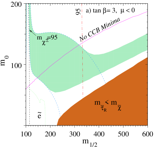
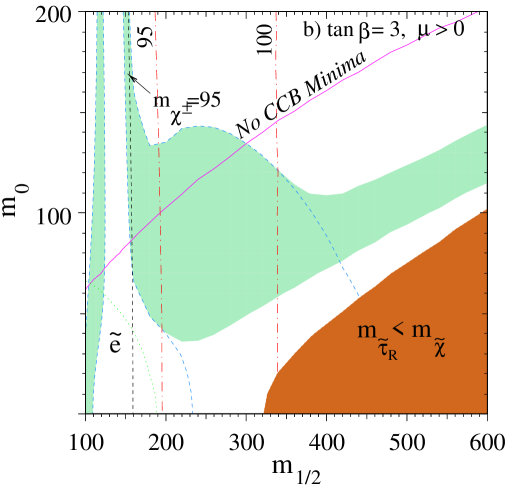
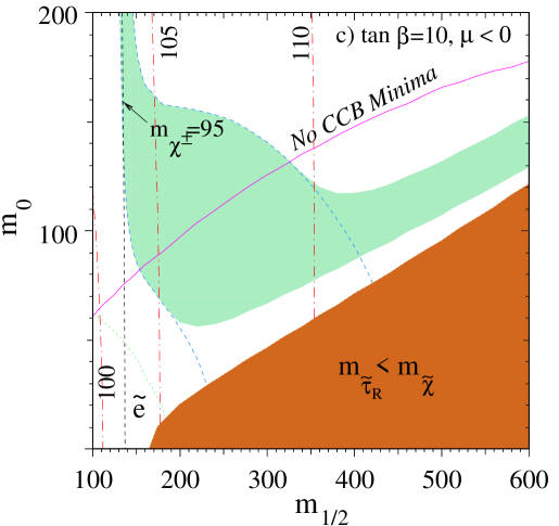
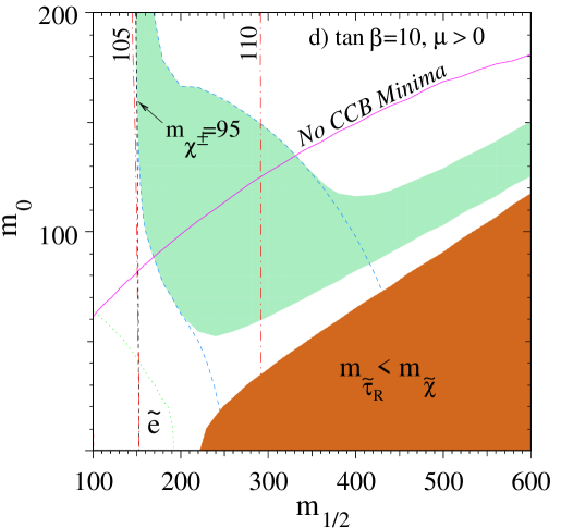
Figure 6: The light-shaded area is the cosmologically preferred region with $0.1\leq\Omega_{\widetilde{\chi}}\,h^{2}\leq 0.3$. The light dashed lines show the location of the cosmologically preferred region if one ignores coannihilations with the light sleptons. In the dark shaded regions in the bottom right of each panel, the LSP is the ${\tilde{\tau}}_{R}$, leading to an unacceptable abundance of charged dark matter. Also shown are the isomass contours $m_{\chi^{\pm}}=95$ GeV and $m_{h}=95,100,105,110$ GeV, as well as an indication of the slepton bound from LEP [31]. In the area below the solid contour, the scalar potential contains charge and/or colour breaking minima.

We also display bounds from LEP particle searches [31] in Fig. 6. The chargino mass bound from LEP essentially saturates the kinematic limit of $\sim 95{\rm\,Ge\kern-1.25ptV}$, modulo a small gap which occurs when the chargino is just slightly heavier than the sneutrino [31]. The chargino $95{\rm\,Ge\kern-1.25ptV}$ isomass contour is displayed as a dark dashed contour, and it cuts off most of the annihilation pole zone, which appears as a chimney in the cosmologically preferred regions at low $m_{1\!/2}$ for the values of $\tan\beta$ considered. Representations of slepton limits from searches [31] for acoplanar lepton pairs at LEP 183 appear as light dotted contours. The most severe experimental constraint at low $\tan\beta$ comes from LEP Higgs searches. At low $\tan\beta$, the tree level light Higgs mass $m_{h}\approx m_{Z}|\cos{2\beta}|$ lies well below the experimental bound $\mathrel{\raise 1.29167pt\hbox{$>$\kern-7.5pt\lower 4.30554pt\hbox{$\sim$}}}95{\rm\,Ge\kern-1.25ptV}$. Radiative corrections to $m_{h}$ are known to be large [29] and increase logarithmically with the stop masses, and hence with $m_{1\!/2}$. Thus, for sufficiently large $m_{1\!/2}$, the Higgs bound may be satisfied. However, if the minimum $m_{1\!/2}$ exceeds its cosmological upper bound for a given $\tan\beta$, this value of $\tan\beta$ is excluded. In the absence of coannihilations, the lower bound on $\tan\beta$ was computed [16] to be 2.0 for $\mu>0$ and 1.65 for $\mu<0$, using mass limits from LEP 183. Higgs isomass contours of 95,100,105, and 110 ${\rm\,Ge\kern-1.25ptV}$ are displayed as dot-dashed lines in Fig. 6.

When we include coannihilations, the cosmological upper bound on $m_{1\!/2}$ weakens considerably, as we have already mentioned. In Fig. 7, we extend the $m_{1\!/2}$ coverage to larger scales, to show the cross-over point between the regions with $\Omega_{\widetilde{\chi}}\,h^{2}<0.3$ and $m_{{\widetilde{\tau}}_{\scriptscriptstyle\rm R}}<m_{\widetilde{\chi}}$. The two constraints together require $m_{1\!/2}\mathrel{\raise 1.29167pt\hbox{$<$\kern-7.5pt\lower 4.30554pt\hbox{$\sim$}}}1450$, corresponding to an upper bound on the neutralino mass of $m_{\widetilde{\chi}}\mathrel{\raise 1.29167pt\hbox{$<$\kern-7.5pt\lower 4.30554pt\hbox{$\sim$}}}600{\rm\,Ge\kern-1.25ptV}$. We take $93{\rm\,Ge\kern-1.25ptV}$ as our experimental lower limit on the Higgs mass, to allow for a $2{\rm\,Ge\kern-1.25ptV}$ uncertainty in the extraction of the radiative corrections to the Higgs mass [29]. The combined lower bound on $\tan\beta$ from the Higgs search and cosmology, including the recent LEP 189 limits, indicates that tan$\beta\mathrel{\raise 1.29167pt\hbox{$>$\kern-7.5pt\lower 4.30554pt\hbox{$\sim$}}}2.2$ for $\mu<0$ and $\mathrel{\raise 1.29167pt\hbox{$>$\kern-7.5pt\lower 4.30554pt\hbox{$\sim$}}}1.8$ for $\mu>0$ .

Figs. 6 and 7 were generated for the particular choice $A_{0}=-m_{1\!/2}$, for reasons described below. Since the stau mass depends weakly on $A_{0}$, particularly at larger values of $\tan\beta$, the position of the $m_{\tilde{\tau}_{R}}=m_{\widetilde{\chi}}$ contour shifts somewhat with $A_{0}$. In Fig. 8, we show figures corresponding to Figs. 6a and 6c for $A_{0}=-3m_{1\!/2}$. For $\tan\beta=3$, the width of the cosmologically allowed band is the same as in Fig. 6a, but the band becomes smaller for $\tan\beta=10$. The effect for positive $A_{0}$ is qualitatively similar. Likewise, varying $A_{0}$ has a tiny effect on the cosmological upper bound on $m_{1\!/2}$ for $\tan\beta=3$, but can produce a small ($\sim 100{\rm\,Ge\kern-1.25ptV}$) reduction in the upper bound for $\tan\beta=10$.

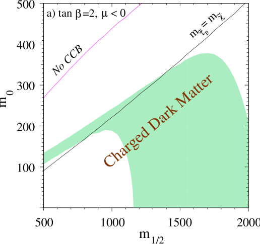
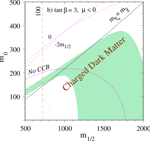
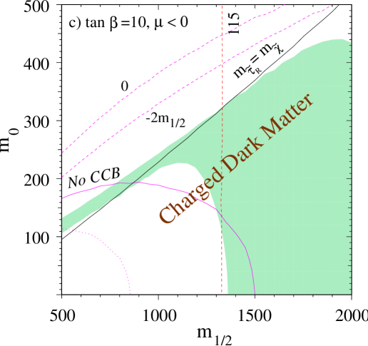
Figure 7: The same as Fig. 6, for $\mu<0$, but extended to larger $m_{1/2}$. The dashed contours in panels b) and c) correspond to the solid CCB line for $A_{0}=0,-2m_{1\!/2}$, and the dotted contour for $m_{t}=170$ GeV.

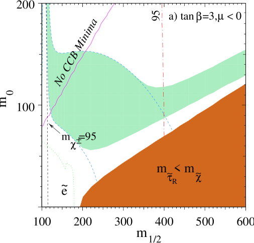
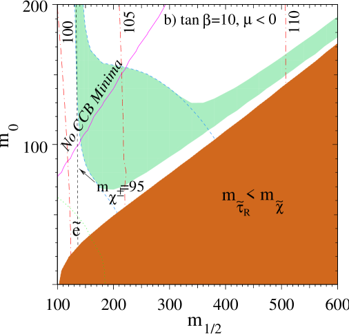
Figure 8: The same as Fig. 6a and Fig. 6c, for $A_{0}=-3m_{1\!/2}$.

Lastly, we show as a dark solid contour the constraint coming from the requirement that the global minimum of the scalar potential not break charge and colour (CCB) [26, 28, 27]. The areas below the light solid line in Figs. 6 and 7 contain charge and/or colour breaking minima, while the regions above the lines are free of such minima, modulo a thin ($\sim 10{\rm\,Ge\kern-1.25ptV}$ wide) strip on top of the solid contour, where local (but not global) CCB minima exist [27]. We have chosen $A_{0}=-m_{1\!/2}$, where the CCB bounds are weakest [26]. The bounds are not strongly dependent on the sign of $\mu$ and are strongest for low $\tan\beta$, where the top Yukawa coupling is largest. In the absence of coannihilations, it is clear from Fig. 6 that a fair fraction of the cosmologically allowed regions contain charge and colour breaking minima. In the presence of coannihilations, the cosmologically allowed region is extended, and as the CCB eventually falls with $m_{1\!/2}$, CCB free regions with small relic densities may occur in the proboscis region as well, particularly at the larger values of $\tan\beta$ considered. In Fig. 7a, we see that, for $\tan\beta=2$, the entire cosmologically allowed region of parameter space also contains CCB minima, even for the conservative choice $A_{0}=-m_{1\!/2}$. For larger $\tan\beta$, the CCB contour bends over and, for $A_{0}=-m_{1\!/2}$, exposes a small strip of the shaded region above the $m_{\tilde{\tau}_{R}}=m_{\widetilde{\chi}}$ line. For comparison, we also show the corresponding CCB contours for $A_{0}=-2m_{1\!/2}$ and 0. For these choices of $A_{0}$, there is again no region which satisfies both the CCB and cosmological constraints. The CCB bounds are also sensitive to the top mass. In Figs. 6 and 7 we have taken $m_{t}=175{\rm\,Ge\kern-1.25ptV}$; taking $m_{t}=170{\rm\,Ge\kern-1.25ptV}$ produces the dotted CCB curves in Fig.7a-c, which expose a much larger piece of the cosmologically allowed band. We recall, however, that a low value of $m_{t}$ also reduces the radiative corrections to the Higgs mass, and therefore makes the Higgs constraint more severe. However, this does not cause a conflict with the cosmological constraints, even for $\tan\beta$ as low as 3.

There is one caveat which one must bear in mind when interpreting the CCB bounds: the tunneling rate from the charge and colour conserving minimum to the CCB minimum is very slow, to such an extent that the conserving minimum is essentially stable over the current lifetime of the universe. Therefore the presence of CCB minima may present more of a cosmological problem of how to populate the physical minimum in preference to the CCB minimum than a constraint on the particle physics [33].

We expect qualitatively similar effects on the corresponding bounds in the MSSM, that is, when we drop the condition of universality of scalar mass at the GUT scale. Though there is an upper limit of ${\cal O}$(a few TeV) for Higgsinos in the MSSM, the limits due to coannihilation that we have been concerned with apply only to the gaugino limit. In this case, one must in general take all the squarks and sleptons degenerate with the neutralino and compute the annihilation and coannihilation cross sections for all possible combinations of sfermions. However, if the rates are the same as for the sleptons, the effect is about a 10-15% decrease in $(\Omega_{\widetilde{\chi}}\,h^{2})^{0}/R$, leading to a similar bound on $m_{\widetilde{\chi}}$ as in the CMSSM. In practice, of course the result will depend on which state is the NLSP.

6 Conclusions and Open Issues

We have documented in this paper the importance of coannihilation effects on the relic density of ${\tilde{B}}$ dark matter. We have presented a general formalism for including their effects in relic density calculations, and have provided (in the Appendix) analytic approximate formulae for many coannihilation processes involving $\tilde{\tau}_{R},{\tilde{e}_{R}}$ and ${\tilde{\mu}_{R}}$ sparticles. We have given in the Figures numerical examples that exhibit their relevance for various values of the CMSSM parameters $m_{1/2},m_{0},A$ and tan$\beta$. We have explained why coannihilation effects are so important, principally because of the $P$-wave suppression of non-relativistic ${\widetilde{\chi}}{\widetilde{\chi}}$ annihilation.

One immediate physical consequence of these coannihilation effects is to relax significantly the previous cosmological upper bound [13] on the LSP mass, from $\mathrel{\raise 1.29167pt\hbox{$>$\kern-7.5pt\lower 4.30554pt\hbox{$\sim$}}}200$ GeV to $\mathrel{\raise 1.29167pt\hbox{$>$\kern-7.5pt\lower 4.30554pt\hbox{$\sim$}}}600$ GeV. This relaxed upper limit could have significant implications for strategies to search for supersymmetric cold dark matter, which have yet to be explored systematically. Coannihilations also allow the LSP mass to approach the boundary of the CMSSM parameter space within which LHC searches for supersymmetry are expected to be sensitive [9]. At first glance, it seems likely that the LHC should still be able to cover all of the CMSSM parameter space that is consistent with supersymmetric cold dark matter, but this point merits further consideration.

Another point to be studied in more detail is the interplay between coannihilation effects and LEP lower limits on sparticle and higgs masses. Previously, limits on $m_{\widetilde{\chi}}$ and tan$\beta$ have been derived from a combination of previous LEP data sets and cosmology [14, 15, 16], but neglecting coannihilation effects. These limits should now be revisited in the light of more recent LEP data [31], as well as coannihilations. We have commented on these questions in this paper, but a complete study lies beyond the scope of the present analysis.

We hope that this paper has not only documented the importance of coannihilation effects, but also provided the reader with the tools needed to join in the exploration of their implications for the interesting open issues raised in the previous paragraph.

Acknowledgments
We are grateful to C. Pallis for pointing out the errors in the Appendix. The work of K.O. was supported in part by DOE grant DE–FG02–94ER–40823. The work of T.F. was supported in part by DOE grant DE–FG02–95ER–40896, and in part by the University of Wisconsin Research Committee with funds granted by the Wisconsin Alumni Research Foundation. The work of M.S. was supported in part by NSF grant PHY–97–22022.

.

Appendix

This section contains simplified formulae for the $\tilde{\tau}\tilde{\tau}^{*},\tilde{\tau}\chi,\tilde{\tau}\tilde{\tau},\tilde{\tau}\tilde{\ell}$ and $\tilde{\tau}\tilde{\ell}^{*}$ annihilation amplitudes, in the $m_{\tilde{\tau}}\rightarrow 0$ limit. Expressions for the $\tilde{\ell}\tilde{\ell}^{*},\tilde{\ell}\tilde{\ell}$ and $\tilde{\ell}\chi$ amplitudes can be obtained by taking $\tau\rightarrow\ell$ in the $\tilde{\tau}\tilde{\tau}^{*},\tilde{\tau}\chi,\tilde{\tau}\tilde{\tau}$ formulae below, and $\tilde{\mu}\tilde{e}$ and $\tilde{e}\tilde{\mu}^{*}$ by taking $\tau\rightarrow e,\ell\rightarrow\mu$ in the $\tilde{\tau}\tilde{\ell}$ and $\tilde{\tau}\tilde{\ell}^{*}$ expressions. The $a$ and $b$ coefficients can be simply numerically extracted from the amplitudes, as described in section 2 of the text.

$\tilde{\tau}\tilde{\tau}^{*}\longrightarrow W^{+}W^{-}$

I. s-channel $H$ annihilation
II. s-channel $h$ annihilation
V. s-channel $Z$ annihilation
VI. s-channel $\gamma$ annihilation

$$f_{1} = (-g_{2}m_{W}\cos(\beta-\alpha))(g_{2}m_{Z}\sin^{2}\!\theta_{\scriptscriptstyle W}\cos(\alpha+\beta)/\cos\theta_{\scriptscriptstyle W})$$

$$f_{2} = (-g_{2}m_{W}\sin(\beta-\alpha))(-g_{2}m_{Z}\sin^{2}\!\theta_{\scriptscriptstyle W}\sin(\alpha+\beta)/\cos\theta_{\scriptscriptstyle W})$$

$$f_{5} = (-g_{2}\sin^{2}\!\theta_{\scriptscriptstyle W}/\cos\theta_{\scriptscriptstyle W})(g_{2}\cos\theta_{\scriptscriptstyle W})$$

$$f_{6} = e^{2}$$

$${\cal T}_{\rm I}\!\!\times\!\!{\cal T}_{\rm I} = (12m_{W}^{4}-4m_{W}^{2}s+s^{2})/(4m_{W}^{4}(m_{H}^{2}-s)^{2})$$

$${\cal T}_{\rm II}\!\!\times\!\!{\cal T}_{\rm II} = (12m_{W}^{4}-4m_{W}^{2}s+s^{2})/(4m_{W}^{4}(m_{h}^{2}-s)^{2})$$

$${\cal T}_{\rm V}\!\!\times\!\!{\cal T}_{\rm V} = (128m_{\tilde{\tau}_{R}}^{2}m_{W}^{4}m_{Z}^{4}s-32m_{\tilde{\tau}_{R}}^{2}m_{W}^{2}m_{Z}^{4}s^{2}-32m_{W}^{4}m_{Z}^{4}s^{2}+8m_{W}^{2}m_{Z}^{4}s^{3}+12m_{W}^{4}m_{Z}^{4}t^{2}-\hfill$$

$$4m_{W}^{2}m_{Z}^{4}st^{2}+m_{Z}^{4}s^{2}t^{2}-24m_{W}^{4}m_{Z}^{4}tu+8m_{W}^{2}m_{Z}^{4}stu-2m_{Z}^{4}s^{2}tu+12m_{W}^{4}m_{Z}^{4}u^{2}-\hfill$$

$$4m_{W}^{2}m_{Z}^{4}su^{2}+m_{Z}^{4}s^{2}u^{2})/(4m_{W}^{4}m_{Z}^{4}(m_{Z}^{2}-s)^{2})$$

$${\cal T}_{\rm VI}\!\!\times\!\!{\cal T}_{\rm VI} = (128m_{\tilde{\tau}_{R}}^{2}m_{W}^{4}s-32m_{\tilde{\tau}_{R}}^{2}m_{W}^{2}s^{2}-32m_{W}^{4}s^{2}+8m_{W}^{2}s^{3}+12m_{W}^{4}t^{2}-4m_{W}^{2}st^{2}+\hfill$$

$$s^{2}t^{2}-24m_{W}^{4}tu+8m_{W}^{2}stu-2s^{2}tu+12m_{W}^{4}u^{2}-4m_{W}^{2}su^{2}+s^{2}u^{2})/(4m_{W}^{4}s^{2})$$

$${\cal T}_{\rm I}\!\!\times\!\!{\cal T}_{\rm II} = (12m_{W}^{4}-4m_{W}^{2}s+s^{2})/(4m_{W}^{4}(m_{H}^{2}-s)(m_{h}^{2}-s))$$

$${\cal T}_{\rm I}\!\!\times\!\!{\cal T}_{\rm V} = (-12m_{W}^{4}m_{Z}^{2}t+m_{Z}^{2}s^{2}t+12m_{W}^{4}m_{Z}^{2}u-m_{Z}^{2}s^{2}u)/(4m_{W}^{4}m_{Z}^{2}(m_{H}^{2}-s)(m_{Z}^{2}-s))$$

$${\cal T}_{\rm II}\!\!\times\!\!{\cal T}_{\rm V} = (-12m_{W}^{4}m_{Z}^{2}t+m_{Z}^{2}s^{2}t+12m_{W}^{4}m_{Z}^{2}u-m_{Z}^{2}s^{2}u)/(4m_{W}^{4}m_{Z}^{2}(m_{h}^{2}-s)(m_{Z}^{2}-s))$$

$${\cal T}_{\rm I}\!\!\times\!\!{\cal T}_{\rm VI} = -(-12m_{W}^{4}t+s^{2}t+12m_{W}^{4}u-s^{2}u)/(4m_{W}^{4}(m_{H}^{2}-s)s)$$

$${\cal T}_{\rm II}\!\!\times\!\!{\cal T}_{\rm VI} = -(-12m_{W}^{4}t+s^{2}t+12m_{W}^{4}u-s^{2}u)/(4m_{W}^{4}(m_{h}^{2}-s)s)$$

$${\cal T}_{\rm V}\!\!\times\!\!{\cal T}_{\rm VI} = (-128m_{\tilde{\tau}_{R}}^{2}m_{W}^{4}m_{Z}^{2}s+32m_{\tilde{\tau}_{R}}^{2}m_{W}^{2}m_{Z}^{2}s^{2}+32m_{W}^{4}m_{Z}^{2}s^{2}-8m_{W}^{2}m_{Z}^{2}s^{3}-\hfill$$

$$12m_{W}^{4}m_{Z}^{2}t^{2}+4m_{W}^{2}m_{Z}^{2}st^{2}-m_{Z}^{2}s^{2}t^{2}+24m_{W}^{4}m_{Z}^{2}tu-8m_{W}^{2}m_{Z}^{2}stu+\hfill$$

$$2m_{Z}^{2}s^{2}tu-12m_{W}^{4}m_{Z}^{2}u^{2}+4m_{W}^{2}m_{Z}^{2}su^{2}-m_{Z}^{2}s^{2}u^{2})/(4m_{W}^{4}m_{Z}^{2}(m_{Z}^{2}-s)s)$$

$$|{\cal T}|^{2} = f_{1}^{2}{\cal T}_{\rm I}\!\!\times\!\!{\cal T}_{\rm I}+f_{2}^{2}{\cal T}_{\rm II}\!\!\times\!\!{\cal T}_{\rm II}+f_{5}^{2}{\cal T}_{\rm V}\!\!\times\!\!{\cal T}_{\rm V}+f_{6}^{2}{\cal T}_{\rm VI}\!\!\times\!\!{\cal T}_{\rm VI}+2f_{1}f_{2}{\cal T}_{\rm I}\!\!\times\!\!{\cal T}_{\rm II}+2f_{1}f_{5}{\cal T}_{\rm I}\!\!\times\!\!{\cal T}_{\rm V}+\hfill$$ (A1)

$$2f_{1}f_{6}{\cal T}_{\rm I}\!\!\times\!\!{\cal T}_{\rm VI}+2f_{2}f_{5}{\cal T}_{\rm II}\!\!\times\!\!{\cal T}_{\rm V}+2f_{2}f_{6}{\cal T}_{\rm II}\!\!\times\!\!{\cal T}_{\rm VI}+2f_{5}f_{6}{\cal T}_{\rm V}\!\!\times\!\!{\cal T}_{\rm VI}$$

$\tilde{\tau}\tilde{\tau}^{*}\longrightarrow ZZ$

I. s-channel $H$ annihilation
II. s-channel $h$ annihilation
III. t-channel $\tilde{\tau}$ exchange
IV. u-channel $\tilde{\tau}$ exchange
V. point interaction

$$f_{1} = (-g_{2}m_{Z}\cos(\beta-\alpha)/\cos\theta_{\scriptscriptstyle W})(g_{2}m_{Z}\sin^{2}\!\theta_{\scriptscriptstyle W}\cos(\alpha+\beta)/\cos\theta_{\scriptscriptstyle W})$$

$$f_{2} = (-g_{2}m_{Z}\sin(\beta-\alpha)/\cos\theta_{\scriptscriptstyle W})(-g_{2}m_{Z}\sin^{2}\!\theta_{\scriptscriptstyle W}\sin(\alpha+\beta)/\cos\theta_{\scriptscriptstyle W})$$

$$f_{3} = (-g_{2}\sin^{2}\!\theta_{\scriptscriptstyle W}/\cos\theta_{\scriptscriptstyle W})^{2}$$

$$f_{4} = (-g_{2}\sin^{2}\!\theta_{\scriptscriptstyle W}/\cos\theta_{\scriptscriptstyle W})^{2}$$

$$f_{5} = -2g_{2}^{2}\sin^{4}\!\theta_{\scriptscriptstyle W}/\cos^{2}\!\theta_{\scriptscriptstyle W}$$

$${\cal T}_{\rm I}\!\!\times\!\!{\cal T}_{\rm I} = (12m_{Z}^{4}-4m_{Z}^{2}s+s^{2})/(4m_{Z}^{4}(m_{H}^{2}-s)^{2})$$

$${\cal T}_{\rm II}\!\!\times\!\!{\cal T}_{\rm II} = (12m_{Z}^{4}-4m_{Z}^{2}s+s^{2})/(4m_{Z}^{4}(m_{h}^{2}-s)^{2})$$

$${\cal T}_{\rm III}\!\!\times\!\!{\cal T}_{\rm III} = (m_{\tilde{\tau}_{R}}^{8}-4m_{\tilde{\tau}_{R}}^{6}m_{Z}^{2}+6m_{\tilde{\tau}_{R}}^{4}m_{Z}^{4}-4m_{\tilde{\tau}_{R}}^{2}m_{Z}^{6}+m_{Z}^{8}-4m_{\tilde{\tau}_{R}}^{6}t+4m_{\tilde{\tau}_{R}}^{4}m_{Z}^{2}t+\hfill$$

$$4m_{\tilde{\tau}_{R}}^{2}m_{Z}^{4}t-4m_{Z}^{6}t+6m_{\tilde{\tau}_{R}}^{4}t^{2}+4m_{\tilde{\tau}_{R}}^{2}m_{Z}^{2}t^{2}+6m_{Z}^{4}t^{2}-4m_{\tilde{\tau}_{R}}^{2}t^{3}-4m_{Z}^{2}t^{3}+t^{4})/\hfill$$

$$(m_{Z}^{4}(m_{\tilde{\tau}_{R}}^{2}-t)^{2})$$

$${\cal T}_{\rm IV}\!\!\times\!\!{\cal T}_{\rm IV} = (m_{\tilde{\tau}_{R}}^{8}-4m_{\tilde{\tau}_{R}}^{6}m_{Z}^{2}+6m_{\tilde{\tau}_{R}}^{4}m_{Z}^{4}-4m_{\tilde{\tau}_{R}}^{2}m_{Z}^{6}+m_{Z}^{8}-4m_{\tilde{\tau}_{R}}^{6}u+4m_{\tilde{\tau}_{R}}^{4}m_{Z}^{2}u+\hfill$$

$$4m_{\tilde{\tau}_{R}}^{2}m_{Z}^{4}u-4m_{Z}^{6}u+6m_{\tilde{\tau}_{R}}^{4}u^{2}+4m_{\tilde{\tau}_{R}}^{2}m_{Z}^{2}u^{2}+6m_{Z}^{4}u^{2}-4m_{\tilde{\tau}_{R}}^{2}u^{3}-4m_{Z}^{2}u^{3}+u^{4})/\hfill$$

$$(m_{Z}^{4}(m_{\tilde{\tau}_{R}}^{2}-u)^{2})$$

$${\cal T}_{\rm V}\!\!\times\!\!{\cal T}_{\rm V} = (12m_{Z}^{4}-4m_{Z}^{2}s+s^{2})/(4m_{Z}^{4})$$

$${\cal T}_{\rm I}\!\!\times\!\!{\cal T}_{\rm II} = (12m_{Z}^{4}-4m_{Z}^{2}s+s^{2})/(4m_{Z}^{4}(m_{H}^{2}-s)(m_{h}^{2}-s))$$

$${\cal T}_{\rm I}\!\!\times\!\!{\cal T}_{\rm III} = (-6m_{\tilde{\tau}_{R}}^{4}m_{Z}^{2}-20m_{\tilde{\tau}_{R}}^{2}m_{Z}^{4}-6m_{Z}^{6}+m_{\tilde{\tau}_{R}}^{4}s+2m_{\tilde{\tau}_{R}}^{2}m_{Z}^{2}s+5m_{Z}^{4}s+8m_{\tilde{\tau}_{R}}^{2}m_{Z}^{2}t+\hfill$$

$$8m_{Z}^{4}t-2m_{\tilde{\tau}_{R}}^{2}st-2m_{Z}^{2}st-2m_{Z}^{2}t^{2}+st^{2}+4m_{\tilde{\tau}_{R}}^{2}m_{Z}^{2}u+4m_{Z}^{4}u-4m_{Z}^{2}tu)/\hfill$$

$$(2m_{Z}^{4}(m_{H}^{2}-s)(m_{\tilde{\tau}_{R}}^{2}-t))$$

$${\cal T}_{\rm I}\!\!\times\!\!{\cal T}_{\rm IV} = (-6m_{\tilde{\tau}_{R}}^{4}m_{Z}^{2}-20m_{\tilde{\tau}_{R}}^{2}m_{Z}^{4}-6m_{Z}^{6}+m_{\tilde{\tau}_{R}}^{4}s+2m_{\tilde{\tau}_{R}}^{2}m_{Z}^{2}s+5m_{Z}^{4}s+4m_{\tilde{\tau}_{R}}^{2}m_{Z}^{2}t+\hfill$$

$$4m_{Z}^{4}t+8m_{\tilde{\tau}_{R}}^{2}m_{Z}^{2}u+8m_{Z}^{4}u-2m_{\tilde{\tau}_{R}}^{2}su-2m_{Z}^{2}su-4m_{Z}^{2}tu-2m_{Z}^{2}u^{2}+su^{2})/\hfill$$

$$(2m_{Z}^{4}(m_{H}^{2}-s)(m_{\tilde{\tau}_{R}}^{2}-u))$$

$${\cal T}_{\rm I}\!\!\times\!\!{\cal T}_{\rm V} = (12m_{Z}^{4}-4m_{Z}^{2}s+s^{2})/(4m_{Z}^{4}(m_{H}^{2}-s))$$

$${\cal T}_{\rm II}\!\!\times\!\!{\cal T}_{\rm III} = (-6m_{\tilde{\tau}_{R}}^{4}m_{Z}^{2}-20m_{\tilde{\tau}_{R}}^{2}m_{Z}^{4}-6m_{Z}^{6}+m_{\tilde{\tau}_{R}}^{4}s+2m_{\tilde{\tau}_{R}}^{2}m_{Z}^{2}s+5m_{Z}^{4}s+8m_{\tilde{\tau}_{R}}^{2}m_{Z}^{2}t+\hfill$$

$$8m_{Z}^{4}t-2m_{\tilde{\tau}_{R}}^{2}st-2m_{Z}^{2}st-2m_{Z}^{2}t^{2}+st^{2}+4m_{\tilde{\tau}_{R}}^{2}m_{Z}^{2}u+4m_{Z}^{4}u-4m_{Z}^{2}tu)/\hfill$$

$$(2m_{Z}^{4}(m_{h}^{2}-s)(m_{\tilde{\tau}_{R}}^{2}-t))$$

$${\cal T}_{\rm II}\!\!\times\!\!{\cal T}_{\rm IV} = (-6m_{\tilde{\tau}_{R}}^{4}m_{Z}^{2}-20m_{\tilde{\tau}_{R}}^{2}m_{Z}^{4}-6m_{Z}^{6}+m_{\tilde{\tau}_{R}}^{4}s+2m_{\tilde{\tau}_{R}}^{2}m_{Z}^{2}s+5m_{Z}^{4}s+4m_{\tilde{\tau}_{R}}^{2}m_{Z}^{2}t+\hfill$$

$$4m_{Z}^{4}t+8m_{\tilde{\tau}_{R}}^{2}m_{Z}^{2}u+8m_{Z}^{4}u-2m_{\tilde{\tau}_{R}}^{2}su-2m_{Z}^{2}su-4m_{Z}^{2}tu-2m_{Z}^{2}u^{2}+su^{2})/\hfill$$

$$(2m_{Z}^{4}(m_{h}^{2}-s)(m_{\tilde{\tau}_{R}}^{2}-u))$$

$${\cal T}_{\rm II}\!\!\times\!\!{\cal T}_{\rm V} = (12m_{Z}^{4}-4m_{Z}^{2}s+s^{2})/(4m_{Z}^{4}(m_{h}^{2}-s))$$

$${\cal T}_{\rm III}\!\!\times\!\!{\cal T}_{\rm IV} = (m_{\tilde{\tau}_{R}}^{8}+12m_{\tilde{\tau}_{R}}^{6}m_{Z}^{2}+38m_{\tilde{\tau}_{R}}^{4}m_{Z}^{4}+12m_{\tilde{\tau}_{R}}^{2}m_{Z}^{6}+m_{Z}^{8}-4m_{\tilde{\tau}_{R}}^{4}m_{Z}^{2}s-24m_{\tilde{\tau}_{R}}^{2}m_{Z}^{4}s-\hfill$$

$$4m_{Z}^{6}s+4m_{Z}^{4}s^{2}-2m_{\tilde{\tau}_{R}}^{6}t-14m_{\tilde{\tau}_{R}}^{4}m_{Z}^{2}t-14m_{\tilde{\tau}_{R}}^{2}m_{Z}^{4}t-2m_{Z}^{6}t+4m_{\tilde{\tau}_{R}}^{2}m_{Z}^{2}st+\hfill$$

$$4m_{Z}^{4}st+m_{\tilde{\tau}_{R}}^{4}t^{2}+2m_{\tilde{\tau}_{R}}^{2}m_{Z}^{2}t^{2}+m_{Z}^{4}t^{2}-2m_{\tilde{\tau}_{R}}^{6}u-14m_{\tilde{\tau}_{R}}^{4}m_{Z}^{2}u-14m_{\tilde{\tau}_{R}}^{2}m_{Z}^{4}u-\hfill$$

$$2m_{Z}^{6}u+4m_{\tilde{\tau}_{R}}^{2}m_{Z}^{2}su+4m_{Z}^{4}su+4m_{\tilde{\tau}_{R}}^{4}tu+16m_{\tilde{\tau}_{R}}^{2}m_{Z}^{2}tu+4m_{Z}^{4}tu-4m_{Z}^{2}stu-\hfill$$

$$2m_{\tilde{\tau}_{R}}^{2}t^{2}u-2m_{Z}^{2}t^{2}u+m_{\tilde{\tau}_{R}}^{4}u^{2}+2m_{\tilde{\tau}_{R}}^{2}m_{Z}^{2}u^{2}+m_{Z}^{4}u^{2}-2m_{\tilde{\tau}_{R}}^{2}tu^{2}-2m_{Z}^{2}tu^{2}+\hfill$$

$$t^{2}u^{2})/(m_{Z}^{4}(m_{\tilde{\tau}_{R}}^{2}-t)(m_{\tilde{\tau}_{R}}^{2}-u))$$

$${\cal T}_{\rm III}\!\!\times\!\!{\cal T}_{\rm V} = (-6m_{\tilde{\tau}_{R}}^{4}m_{Z}^{2}-20m_{\tilde{\tau}_{R}}^{2}m_{Z}^{4}-6m_{Z}^{6}+m_{\tilde{\tau}_{R}}^{4}s+2m_{\tilde{\tau}_{R}}^{2}m_{Z}^{2}s+5m_{Z}^{4}s+8m_{\tilde{\tau}_{R}}^{2}m_{Z}^{2}t+\hfill$$

$$8m_{Z}^{4}t-2m_{\tilde{\tau}_{R}}^{2}st-2m_{Z}^{2}st-2m_{Z}^{2}t^{2}+st^{2}+4m_{\tilde{\tau}_{R}}^{2}m_{Z}^{2}u+4m_{Z}^{4}u-4m_{Z}^{2}tu)/\hfill$$

$$(2m_{Z}^{4}(m_{\tilde{\tau}_{R}}^{2}-t))$$

$${\cal T}_{\rm IV}\!\!\times\!\!{\cal T}_{\rm V} = (-6m_{\tilde{\tau}_{R}}^{4}m_{Z}^{2}-20m_{\tilde{\tau}_{R}}^{2}m_{Z}^{4}-6m_{Z}^{6}+m_{\tilde{\tau}_{R}}^{4}s+2m_{\tilde{\tau}_{R}}^{2}m_{Z}^{2}s+5m_{Z}^{4}s+4m_{\tilde{\tau}_{R}}^{2}m_{Z}^{2}t+\hfill$$

$$4m_{Z}^{4}t+8m_{\tilde{\tau}_{R}}^{2}m_{Z}^{2}u+8m_{Z}^{4}u-2m_{\tilde{\tau}_{R}}^{2}su-2m_{Z}^{2}su-4m_{Z}^{2}tu-2m_{Z}^{2}u^{2}+su^{2})/\hfill$$

$$(2m_{Z}^{4}(m_{\tilde{\tau}_{R}}^{2}-u))$$

$$|{\cal T}|^{2} = f_{1}^{2}{\cal T}_{\rm I}\!\!\times\!\!{\cal T}_{\rm I}+f_{2}^{2}{\cal T}_{\rm II}\!\!\times\!\!{\cal T}_{\rm II}+f_{3}^{2}{\cal T}_{\rm III}\!\!\times\!\!{\cal T}_{\rm III}+f_{4}^{2}{\cal T}_{\rm IV}\!\!\times\!\!{\cal T}_{\rm IV}+f_{5}^{2}{\cal T}_{\rm V}\!\!\times\!\!{\cal T}_{\rm V}+2f_{1}f_{2}{\cal T}_{\rm I}\!\!\times\!\!{\cal T}_{\rm II}+\hfill$$ (A2)

$$2f_{1}f_{3}{\cal T}_{\rm I}\!\!\times\!\!{\cal T}_{\rm III}+2f_{1}f_{4}{\cal T}_{\rm I}\!\!\times\!\!{\cal T}_{\rm IV}+2f_{1}f_{5}{\cal T}_{\rm I}\!\!\times\!\!{\cal T}_{\rm V}+2f_{2}f_{3}{\cal T}_{\rm II}\!\!\times\!\!{\cal T}_{\rm III}+2f_{2}f_{4}{\cal T}_{\rm II}\!\!\times\!\!{\cal T}_{\rm IV}+\hfill$$

$$2f_{2}f_{5}{\cal T}_{\rm II}\!\!\times\!\!{\cal T}_{\rm V}+2f_{3}f_{4}{\cal T}_{\rm III}\!\!\times\!\!{\cal T}_{\rm IV}+2f_{3}f_{5}{\cal T}_{\rm III}\!\!\times\!\!{\cal T}_{\rm V}+2f_{4}f_{5}{\cal T}_{\rm IV}\!\!\times\!\!{\cal T}_{\rm V}$$

$\tilde{\tau}\tilde{\tau}^{*}\longrightarrow Z\gamma$

I. t-channel $\tilde{\tau}$ exchange
II. u-channel $\tilde{\tau}$ exchange
III. point interaction

$$f_{1} = e(-g_{2}\sin^{2}\!\theta_{\scriptscriptstyle W}/\cos\theta_{\scriptscriptstyle W})$$

$$f_{2} = e(-g_{2}\sin^{2}\!\theta_{\scriptscriptstyle W}/\cos\theta_{\scriptscriptstyle W})$$

$$f_{3} = 2eg_{2}\sin^{2}\!\theta_{\scriptscriptstyle W}/\cos\theta_{\scriptscriptstyle W}$$

$${\cal T}_{\rm I}\!\!\times\!\!{\cal T}_{\rm I} = (-2m_{\tilde{\tau}_{R}}^{6}+4m_{\tilde{\tau}_{R}}^{4}m_{Z}^{2}-2m_{\tilde{\tau}_{R}}^{2}m_{Z}^{4}+2m_{\tilde{\tau}_{R}}^{4}t+8m_{\tilde{\tau}_{R}}^{2}m_{Z}^{2}t-2m_{Z}^{4}t+2m_{\tilde{\tau}_{R}}^{2}t^{2}+\hfill$$

$$4m_{Z}^{2}t^{2}-2t^{3})/(m_{Z}^{2}(m_{\tilde{\tau}_{R}}^{2}-t)^{2})$$

$${\cal T}_{\rm II}\!\!\times\!\!{\cal T}_{\rm II} = (-2m_{\tilde{\tau}_{R}}^{6}+4m_{\tilde{\tau}_{R}}^{4}m_{Z}^{2}-2m_{\tilde{\tau}_{R}}^{2}m_{Z}^{4}+2m_{\tilde{\tau}_{R}}^{4}u-8m_{\tilde{\tau}_{R}}^{2}m_{Z}^{2}u-2m_{Z}^{4}u+2m_{\tilde{\tau}_{R}}^{2}u^{2}+\hfill$$

$$4m_{Z}^{2}u^{2}-2u^{3})/(m_{Z}^{2}(m_{\tilde{\tau}_{R}}^{2}-u)^{2})$$

$${\cal T}_{\rm III}\!\!\times\!\!{\cal T}_{\rm III} = 3$$

$${\cal T}_{\rm I}\!\!\times\!\!{\cal T}_{\rm II} = (6m_{\tilde{\tau}_{R}}^{6}+36m_{\tilde{\tau}_{R}}^{4}m_{Z}^{2}+6m_{\tilde{\tau}_{R}}^{2}m_{Z}^{4}-2m_{\tilde{\tau}_{R}}^{4}s-24m_{\tilde{\tau}_{R}}^{2}m_{Z}^{2}s-2m_{Z}^{4}s+4m_{Z}^{2}s^{2}-\hfill$$

$$7m_{\tilde{\tau}_{R}}^{4}t-12m_{\tilde{\tau}_{R}}^{2}m_{Z}^{2}t-m_{Z}^{4}t+2m_{\tilde{\tau}_{R}}^{2}st+4m_{Z}^{2}st+m_{\tilde{\tau}_{R}}^{2}t^{2}+m_{Z}^{2}t^{2}-7m_{\tilde{\tau}_{R}}^{4}u-\hfill$$

$$12m_{\tilde{\tau}_{R}}^{2}m_{Z}^{2}u-m_{Z}^{4}u+2m_{\tilde{\tau}_{R}}^{2}su+4m_{Z}^{2}su+8m_{\tilde{\tau}_{R}}^{2}tu+2m_{Z}^{2}tu-2stu-t^{2}u\hfill$$

$$+m_{\tilde{\tau}_{R}}^{2}u^{2}+m_{Z}^{2}u^{2}-tu^{2})/(m_{Z}^{2}(m_{\tilde{\tau}_{R}}^{2}-t)(m_{\tilde{\tau}_{R}}^{2}-u))$$

$${\cal T}_{\rm I}\!\!\times\!\!{\cal T}_{\rm III} = (-2m_{\tilde{\tau}_{R}}^{4}-15m_{\tilde{\tau}_{R}}^{2}m_{Z}^{2}-3m_{Z}^{4}+m_{\tilde{\tau}_{R}}^{2}s+5m_{Z}^{2}s+2m_{\tilde{\tau}_{R}}^{2}t+3m_{Z}^{2}t-st+\hfill$$

$$2m_{\tilde{\tau}_{R}}^{2}u+4m_{Z}^{2}u-2tu)/(2m_{Z}^{2}(m_{\tilde{\tau}_{R}}^{2}-t))$$

$${\cal T}_{\rm II}\!\!\times\!\!{\cal T}_{\rm III} = (-2m_{\tilde{\tau}_{R}}^{4}-15m_{\tilde{\tau}_{R}}^{2}m_{Z}^{2}-3m_{Z}^{4}+m_{\tilde{\tau}_{R}}^{2}s+5m_{Z}^{2}s+2m_{\tilde{\tau}_{R}}^{2}t+4m_{Z}^{2}t+2m_{\tilde{\tau}_{R}}^{2}u+\hfill$$

$$3m_{Z}^{2}u-su-2tu)/(2m_{Z}^{2}(m_{\tilde{\tau}_{R}}^{2}-u))$$

$$|{\cal T}|^{2} = f_{1}^{2}{\cal T}_{\rm I}\!\!\times\!\!{\cal T}_{\rm I}+f_{2}^{2}{\cal T}_{\rm II}\!\!\times\!\!{\cal T}_{\rm II}+f_{3}^{2}{\cal T}_{\rm III}\!\!\times\!\!{\cal T}_{\rm III}+2f_{1}f_{2}{\cal T}_{\rm I}\!\!\times\!\!{\cal T}_{\rm II}+2f_{1}f_{3}{\cal T}_{\rm I}\!\!\times\!\!{\cal T}_{\rm III}+\hfill$$ (A3)

$$2f_{2}f_{3}{\cal T}_{\rm II}\!\!\times\!\!{\cal T}_{\rm III}$$

$\tilde{\tau}\tilde{\tau}^{*}\longrightarrow\gamma\gamma$

I. t-channel $\tilde{\tau}$ exchange
II. u-channel $\tilde{\tau}$ exchange
III. point interaction

$$f_{1} = e^{2}$$

$$f_{2} = e^{2}$$

$$f_{3} = -2e^{2}$$

$${\cal T}_{\rm I}\!\!\times\!\!{\cal T}_{\rm I} = (4m_{\tilde{\tau}_{R}}^{4}+8m_{\tilde{\tau}_{R}}^{2}t+4t^{2})/(m_{\tilde{\tau}_{R}}^{2}-t)^{2}$$

$${\cal T}_{\rm II}\!\!\times\!\!{\cal T}_{\rm II} = (4m_{\tilde{\tau}_{R}}^{4}+8m_{\tilde{\tau}_{R}}^{2}u+4u^{2})/(m_{\tilde{\tau}_{R}}^{2}-u)^{2}$$

$${\cal T}_{\rm III}\!\!\times\!\!{\cal T}_{\rm III} = 4$$

$${\cal T}_{\rm I}\!\!\times\!\!{\cal T}_{\rm II} = (36m_{\tilde{\tau}_{R}}^{4}-24m_{\tilde{\tau}_{R}}^{2}s+4s^{2}-12m_{\tilde{\tau}_{R}}^{2}t+4st+t^{2}-12m_{\tilde{\tau}_{R}}^{2}u+4su+2tu+u^{2})/\hfill$$

$$((m_{\tilde{\tau}_{R}}^{2}-t)(m_{\tilde{\tau}_{R}}^{2}-u))$$

$${\cal T}_{\rm I}\!\!\times\!\!{\cal T}_{\rm III} = (-12m_{\tilde{\tau}_{R}}^{2}+5s+4u)/(2(m_{\tilde{\tau}_{R}}^{2}-t))$$

$${\cal T}_{\rm II}\!\!\times\!\!{\cal T}_{\rm III} = (-12m_{\tilde{\tau}_{R}}^{2}+5s+4t)/(2(m_{\tilde{\tau}_{R}}^{2}-u))$$

$$|{\cal T}|^{2} = f_{1}^{2}{\cal T}_{\rm I}\!\!\times\!\!{\cal T}_{\rm I}+f_{2}^{2}{\cal T}_{\rm II}\!\!\times\!\!{\cal T}_{\rm II}+f_{3}^{2}{\cal T}_{\rm III}\!\!\times\!\!{\cal T}_{\rm III}+2f_{1}f_{2}{\cal T}_{\rm I}\!\!\times\!\!{\cal T}_{\rm II}+2f_{1}f_{3}{\cal T}_{\rm I}\!\!\times\!\!{\cal T}_{\rm III}+\hfill$$ (A4)

$$2f_{2}f_{3}{\cal T}_{\rm II}\!\!\times\!\!{\cal T}_{\rm III}$$

$\tilde{\tau}\tilde{\tau}^{*}\longrightarrow Zh[H]$

I. t-channel $\tilde{\tau}$ exchange
II. u-channel $\tilde{\tau}$ exchange
III. s-channel $Z$ annihilation

$$f_{1} = (-g_{2}\sin^{2}\!\theta_{\scriptscriptstyle W}/\cos\theta_{\scriptscriptstyle W})(-g_{2}m_{Z}\sin^{2}\!\theta_{\scriptscriptstyle W}\sin[-\cos](\alpha+\beta)/\cos\theta_{\scriptscriptstyle W})$$

$$f_{2} = -(-g_{2}\sin^{2}\!\theta_{\scriptscriptstyle W}/\cos\theta_{\scriptscriptstyle W})(-g_{2}m_{Z}\sin^{2}\!\theta_{\scriptscriptstyle W}\sin[-\cos](\alpha+\beta)/\cos\theta_{\scriptscriptstyle W})$$

$$f_{3} = (-g_{2}\sin^{2}\!\theta_{\scriptscriptstyle W}/\cos\theta_{\scriptscriptstyle W})(-g_{2}m_{Z}\sin[\cos](\beta-\alpha)/\cos\theta_{\scriptscriptstyle W})$$

$${\cal T}_{\rm I}\!\!\times\!\!{\cal T}_{\rm I} = (m_{\tilde{\tau}_{R}}^{4}+(m_{Z}^{2}-t)^{2}-2m_{\tilde{\tau}_{R}}^{2}(m_{Z}^{2}+t))/(m_{Z}^{2}(m_{\tilde{\tau}_{R}}^{2}-t)^{2})$$

$${\cal T}_{\rm II}\!\!\times\!\!{\cal T}_{\rm II} = (m_{\tilde{\tau}_{R}}^{4}+(m_{Z}^{2}-u)^{2}-2m_{\tilde{\tau}_{R}}^{2}(m_{Z}^{2}+u))/(m_{Z}^{2}(m_{\tilde{\tau}_{R}}^{2}-u)^{2})$$

$${\cal T}_{\rm I}\!\!\times\!\!{\cal T}_{\rm II} = (m_{\tilde{\tau}_{R}}^{4}+m_{Z}^{4}+m_{\tilde{\tau}_{R}}^{2}(6m_{Z}^{2}-t-u)+tu-m_{Z}^{2}(2s+t+u))/\hfill$$

$$(m_{Z}^{2}(m_{\tilde{\tau}_{R}}^{2}-t)(m_{\tilde{\tau}_{R}}^{2}-u))$$

$${\cal T}_{\rm I}\!\!\times\!\!{\cal T}_{\rm III} = (t(t-u)+m_{\tilde{\tau}_{R}}^{2}(-8m_{Z}^{2}-t+u)+m_{Z}^{2}(2s-t+u))/\hfill$$

$$(2m_{Z}^{2}(m_{Z}^{2}-s)(m_{\tilde{\tau}_{R}}^{2}-t))$$

$${\cal T}_{\rm II}\!\!\times\!\!{\cal T}_{\rm III} = ((t-u)u+m_{\tilde{\tau}_{R}}^{2}(8m_{Z}^{2}-t+u)+m_{Z}^{2}(-2s-t+u))/\hfill$$

$$(2m_{Z}^{2}(m_{Z}^{2}-s)(m_{\tilde{\tau}_{R}}^{2}-u))$$

$${\cal T}_{\rm III}\!\!\times\!\!{\cal T}_{\rm III} = (-16m_{\tilde{\tau}_{R}}^{2}m_{Z}^{2}+4m_{Z}^{2}s+(t-u)^{2})/(4m_{Z}^{2}(m_{Z}^{2}-s)^{2})$$

$$|{\cal T}|^{2} = f_{1}^{2}{\cal T}_{\rm I}\!\!\times\!\!{\cal T}_{\rm I}+f_{2}^{2}{\cal T}_{\rm II}\!\!\times\!\!{\cal T}_{\rm II}+f_{3}^{2}{\cal T}_{\rm III}\!\!\times\!\!{\cal T}_{\rm III}+2f_{1}f_{2}{\cal T}_{\rm I}\!\!\times\!\!{\cal T}_{\rm II}+2f_{1}f_{3}{\cal T}_{\rm I}\!\!\times\!\!{\cal T}_{\rm III}+\hfill$$ (A5)

$$2f_{2}f_{3}{\cal T}_{\rm II}\!\!\times\!\!{\cal T}_{\rm III}$$

$\tilde{\tau}\tilde{\tau}^{*}\longrightarrow\gamma h[H]$

I. t-channel $\tilde{\tau}$ exchange
II. u-channel $\tilde{\tau}$ exchange

$$f_{1} = (e)(-g_{2}m_{Z}\sin^{2}\!\theta_{\scriptscriptstyle W}\sin[-\cos](\alpha+\beta)/\cos\theta_{\scriptscriptstyle W})$$

$$f_{2} = -(e)(-g_{2}m_{Z}\sin^{2}\!\theta_{\scriptscriptstyle W}\sin[-\cos](\alpha+\beta)/\cos\theta_{\scriptscriptstyle W})$$

$${\cal T}_{\rm I}\!\!\times\!\!{\cal T}_{\rm I} = -2(m_{\tilde{\tau}_{R}}^{2}+t)/(m_{\tilde{\tau}_{R}}^{2}-t)^{2}$$

$${\cal T}_{\rm I}\!\!\times\!\!{\cal T}_{\rm II} = -(-6m_{\tilde{\tau}_{R}}^{2}+2s+t+u)/((m_{\tilde{\tau}_{R}}^{2}-t)(m_{\tilde{\tau}_{R}}^{2}-u))$$

$${\cal T}_{\rm II}\!\!\times\!\!{\cal T}_{\rm II} = -2(m_{\tilde{\tau}_{R}}^{2}+u)/(m_{\tilde{\tau}_{R}}^{2}-u)^{2}$$

$$|{\cal T}|^{2} = f_{1}^{2}{\cal T}_{\rm I}\!\!\times\!\!{\cal T}_{\rm I}+f_{2}^{2}{\cal T}_{\rm II}\!\!\times\!\!{\cal T}_{\rm II}+2f_{1}f_{2}{\cal T}_{\rm I}\!\!\times\!\!{\cal T}_{\rm II}$$ (A6)

$\tilde{\tau}\tilde{\tau}^{*}\longrightarrow ZA$

I. s-channel $h$ exchange
II. s-channel $H$ exchange

$$f_{1} = (g_{2}\cos(\alpha-\beta)/(2\cos\theta_{\scriptscriptstyle W})(-g_{2}m_{Z}\sin^{2}\!\theta_{\scriptscriptstyle W}\sin(\alpha+\beta)/\cos\theta_{\scriptscriptstyle W})$$

$$f_{2} = (g_{2}\sin(\alpha-\beta)/(2\cos\theta_{\scriptscriptstyle W})(g_{2}m_{Z}\sin^{2}\!\theta_{\scriptscriptstyle W}\cos(\alpha+\beta)/\cos\theta_{\scriptscriptstyle W})$$

$${\cal T}_{\rm I}\!\!\times\!\!{\cal T}_{\rm I} = (m_{A}^{4}+(m_{Z}^{2}-s)^{2}-2m_{A}^{2}(m_{Z}^{2}+s))/(m_{Z}^{2}(m_{h}^{2}-s)^{2})$$

$${\cal T}_{\rm II}\!\!\times\!\!{\cal T}_{\rm II} = (m_{A}^{4}+(m_{Z}^{2}-s)^{2}-2m_{A}^{2}(m_{Z}^{2}+s))/(m_{Z}^{2}(m_{H}^{2}-s)^{2})$$

$${\cal T}_{\rm I}\!\!\times\!\!{\cal T}_{\rm II} = (m_{A}^{4}+(m_{Z}^{2}-s)^{2}-2m_{A}^{2}(m_{Z}^{2}+s)/(m_{Z}^{2}(m_{H}^{2}-s)(m_{h}^{2}-s)))$$

$$|{\cal T}|^{2} = f_{1}^{2}{\cal T}_{\rm I}\!\!\times\!\!{\cal T}_{\rm I}+f_{2}^{2}{\cal T}_{\rm II}\!\!\times\!\!{\cal T}_{\rm II}+2f_{1}f_{2}{\cal T}_{\rm I}\!\!\times\!\!{\cal T}_{\rm II}$$ (A7)

$\tilde{\tau}\tilde{\tau}^{*}\longrightarrow\tau\bar{\tau}$

III. s-channel $Z$ annihilation
IV. s-channel $\gamma$ annihilation
V. t-channel $\chi$ exchange

$$f_{3c} = (-g_{2}\sin^{2}\!\theta_{\scriptscriptstyle W}/\cos\theta_{\scriptscriptstyle W})(g_{2}(1-4\sin^{2}\!\theta_{\scriptscriptstyle W})/(4\cos\!\theta_{\scriptscriptstyle W}))$$

$$f_{3d} = (-g_{2}\sin^{2}\!\theta_{\scriptscriptstyle W}/\cos\theta_{\scriptscriptstyle W})(-g_{2}/(4\cos\!\theta_{\scriptscriptstyle W}))$$

$$f_{4c} = e^{2}$$

$$K = g_{1}N_{i1}/\sqrt{2}$$

$$K^{\prime} = g_{1}N_{j1}/\sqrt{2}$$

$${\cal T}_{\rm III}\!\!\times\!\!{\cal T}_{\rm III} = 2(-4f_{3c}^{2}m_{\tilde{\tau}_{R}}^{2}s-4f_{3d}^{2}m_{\tilde{\tau}_{R}}^{2}sf_{3c}^{2}s^{2}+f_{3d}^{2}s^{2}-f_{3c}^{2}t^{2}-f_{3d}^{2}t^{2}+2f_{3c}^{2}tu+2f_{3d}^{2}tu-\hfill$$

$$f_{3c}^{2}u^{2}-f_{3d}^{2}u^{2})/(m_{Z}^{2}-s)^{2}$$

$${\cal T}_{\rm III}\!\!\times\!\!{\cal T}_{\rm IV} = 2f_{3c}f_{4c}(4m_{\tilde{\tau}_{R}}^{2}s-s^{2}+t^{2}-2tu+u^{2})/((m_{Z}^{2}-s)s)$$

$${\cal T}_{\rm IV}\!\!\times\!\!{\cal T}_{\rm IV} = 2f_{4c}^{2}(-4m_{\tilde{\tau}_{R}}^{2}s+s^{2}-t^{2}+2tu-u^{2})/s^{2}$$

$${\cal T}_{\rm III}\!\!\times\!\!{\cal T}_{\rm V} = -2(f_{3c}+f_{3d})K^{2}(4m_{\tilde{\tau}_{R}}^{2}s-s^{2}+(t-u)^{2})/((m_{Z}^{2}-s)({m_{\tilde{\chi}}}_{i}^{2}-t))$$

$${\cal T}_{\rm IV}\!\!\times\!\!{\cal T}_{\rm V} = 2(f_{4c})K^{2}(4m_{\tilde{\tau}_{R}}^{2}s-s^{2}+(t-u)^{2})/(s({m_{\tilde{\chi}}}_{i}^{2}-t))$$

$${\cal T}_{\rm V}\!\!\times\!\!{\cal T}_{\rm V} = (16K^{2}K^{\prime 2}(m_{\tilde{\tau}_{R}}^{4}-tu))/(({m_{\tilde{\chi}}}_{i}^{2}-t)(-{m_{\tilde{\chi}}}_{j}^{2}+t))$$

$$|{\cal T}|^{2} = {\cal T}_{\rm III}\!\!\times\!\!{\cal T}_{\rm III}+{\cal T}_{\rm IV}\!\!\times\!\!{\cal T}_{\rm IV}+2{\cal T}_{\rm III}\!\!\times\!\!{\cal T}_{\rm IV}+\hfill$$ (A8)

$$\sum_{i,j=1}^{4}\left(({\cal T}_{\rm I}\!\!\times\!\!{\cal T}_{\rm V}+{\cal T}_{\rm II}\!\!\times\!\!{\cal T}_{\rm V}+{\cal T}_{\rm III}\!\!\times\!\!{\cal T}_{\rm V}+{\cal T}_{\rm IV}\!\!\times\!\!{\cal T}_{\rm V})/2+{\cal T}_{\rm V}\!\!\times\!\!{\cal T}_{\rm V}\right)$$

$\tilde{\tau}\tilde{\tau}^{*}\longrightarrow f\!\bar{f}$

III. s-channel $Z$ annihilation
IV. s-channel $\gamma$ annihilation

$$f_{3c} = (-g_{2}\sin^{2}\!\theta_{\scriptscriptstyle W}/\cos\theta_{\scriptscriptstyle W})(g_{2}(-2T_{3}^{f}+4Q_{f}\sin^{2}\!\theta_{\scriptscriptstyle W})/(4\cos\!\theta_{\scriptscriptstyle W}))$$

$$f_{3d} = (-g_{2}\sin^{2}\!\theta_{\scriptscriptstyle W}/\cos\theta_{\scriptscriptstyle W})(g_{2}(2T_{3}^{f})/(4\cos\!\theta_{\scriptscriptstyle W}))$$

$$f_{4c} = -e_{f}e^{2}$$

$${\cal T}_{\rm III}\!\!\times\!\!{\cal T}_{\rm III} = 2(16f_{3d}^{2}m_{\tilde{\tau}_{R}}^{2}m_{f}^{2}-4f_{3c}^{2}m_{\tilde{\tau}_{R}}^{2}s-4f_{3d}^{2}m_{\tilde{\tau}_{R}}^{2}s-4f_{3d}^{2}m_{f}^{2}s+f_{3c}^{2}s^{2}+f_{3d}^{2}s^{2}-\hfill$$

$$f_{3c}^{2}t^{2}-f_{3d}^{2}t^{2}+2f_{3c}^{2}tu+2f_{3d}^{2}tu-f_{3c}^{2}u^{2}-f_{3d}^{2}u^{2})/(m_{Z}^{2}-s)^{2}$$

$${\cal T}_{\rm III}\!\!\times\!\!{\cal T}_{\rm IV} = 2f_{3c}f_{4c}(4m_{\tilde{\tau}_{R}}^{2}s-s^{2}+t^{2}-2tu+u^{2})/((m_{Z}^{2}-s)s)$$

$${\cal T}_{\rm IV}\!\!\times\!\!{\cal T}_{\rm IV} = 2f_{4c}^{2}(-4m_{\tilde{\tau}_{R}}^{2}s+s^{2}-t^{2}+2tu-u^{2})/s^{2}$$

$$|{\cal T}|^{2} = ({\cal T}_{\rm III}\!\!\times\!\!{\cal T}_{\rm III}+{\cal T}_{\rm IV}\!\!\times\!\!{\cal T}_{\rm IV}+2{\cal T}_{\rm III}\!\!\times\!\!{\cal T}_{\rm IV})(\times 3\;{\rm for\;quarks})$$ (A9)

$\tilde{\tau}\tilde{\tau}^{*}\longrightarrow t\bar{t}$

I . s-channel $H$ annihilation
II. s-channel $h$ annihilation
III. s-channel $Z$ annihilation
IV. s-channel $\gamma$ annihilation

$$f_{1a} = (g_{2}m_{Z}\sin^{2}\!\theta_{\scriptscriptstyle W}\cos(\alpha+\beta)/\cos\theta_{\scriptscriptstyle W})(-g_{2}m_{t}\sin\alpha/(2m_{W}\sin\beta))$$

$$f_{2a} = (-g_{2}m_{Z}\sin^{2}\!\theta_{\scriptscriptstyle W}\sin(\alpha+\beta)/\cos\theta_{\scriptscriptstyle W})(-g_{2}m_{t}\cos\alpha/(2m_{W}\sin\beta))$$

$$f_{3c} = (-g_{2}\sin^{2}\!\theta_{\scriptscriptstyle W}/\cos\theta_{\scriptscriptstyle W})(g_{2}(-1+4Q_{t}\sin^{2}\!\theta_{\scriptscriptstyle W})/(4\cos\!\theta_{\scriptscriptstyle W}))$$

$$f_{3d} = (-g_{2}\sin^{2}\!\theta_{\scriptscriptstyle W}/\cos\theta_{\scriptscriptstyle W})(g_{2}/(4\cos\!\theta_{\scriptscriptstyle W}))$$

$$f_{4c} = -e_{t}e^{2}$$

$${\cal T}_{\rm I}\!\!\times\!\!{\cal T}_{\rm I} = 2f_{1a}^{2}(-4m_{t}^{2}+s)/(-m_{H}^{2}+s)^{2}$$

$${\cal T}_{\rm II}\!\!\times\!\!{\cal T}_{\rm II} = 2f_{2a}^{2}(-4m_{t}^{2}+s)/(-m_{h}^{2}+s)^{2}$$

$${\cal T}_{\rm III}\!\!\times\!\!{\cal T}_{\rm III} = 2(16f_{3d}^{2}m_{\tilde{\tau}_{R}}^{2}m_{t}^{2}-4f_{3c}^{2}m_{\tilde{\tau}_{R}}^{2}s-4f_{3d}^{2}m_{\tilde{\tau}_{R}}^{2}s-4f_{3d}^{2}m_{t}^{2}s+f_{3c}^{2}s^{2}+f_{3d}^{2}s^{2}-\hfill$$

$$f_{3c}^{2}t^{2}-f_{3d}^{2}t^{2}+2f_{3c}^{2}tu+2f_{3d}^{2}tu-f_{3c}^{2}u^{2}-f_{3d}^{2}u^{2})/(m_{Z}^{2}-s)^{2}$$

$${\cal T}_{\rm I}\!\!\times\!\!{\cal T}_{\rm II} = 2f_{1a}f_{2a}(-4m_{t}^{2}+s)/((-m_{H}^{2}+s)(-m_{h}^{2}+s))$$

$${\cal T}_{\rm I}\!\!\times\!\!{\cal T}_{\rm III} = 4f_{1a}f_{3c}m_{t}(t-u)/((m_{H}^{2}-s)(-m_{Z}^{2}+s))$$

$${\cal T}_{\rm II}\!\!\times\!\!{\cal T}_{\rm III} = 4f_{2a}f_{3c}m_{t}(t-u)/((m_{h}^{2}-s)(-m_{Z}^{2}+s))$$

$${\cal T}_{\rm I}\!\!\times\!\!{\cal T}_{\rm IV} = 4f_{1a}f_{4c}m_{t}(t-u)/((m_{H}^{2}-s)s)$$

$${\cal T}_{\rm II}\!\!\times\!\!{\cal T}_{\rm IV} = 4f_{2a}f_{4c}m_{t}(t-u)/((m_{h}^{2}-s)s)$$

$${\cal T}_{\rm III}\!\!\times\!\!{\cal T}_{\rm IV} = 2f_{3c}f_{4c}(4m_{\tilde{\tau}_{R}}^{2}s-s^{2}+t^{2}-2tu+u^{2})/((m_{Z}^{2}-s)s)$$

$${\cal T}_{\rm IV}\!\!\times\!\!{\cal T}_{\rm IV} = 2f_{4c}^{2}(-4m_{\tilde{\tau}_{R}}^{2}s+s^{2}-t^{2}+2tu-u^{2})/s^{2}$$

$$|{\cal T}|^{2} = 3\;({\cal T}_{\rm I}\!\!\times\!\!{\cal T}_{\rm I}+{\cal T}_{\rm II}\!\!\times\!\!{\cal T}_{\rm II}+{\cal T}_{\rm III}\!\!\times\!\!{\cal T}_{\rm III}+{\cal T}_{\rm IV}\!\!\times\!\!{\cal T}_{\rm IV}+2{\cal T}_{\rm I}\!\!\times\!\!{\cal T}_{\rm II}+2{\cal T}_{\rm I}\!\!\times\!\!{\cal T}_{\rm III}+2{\cal T}_{\rm I}\!\!\times\!\!{\cal T}_{\rm IV}+\hfill$$ (A10)

$$2{\cal T}_{\rm II}\!\!\times\!\!{\cal T}_{\rm III}+2{\cal T}_{\rm II}\!\!\times\!\!{\cal T}_{\rm IV}+2{\cal T}_{\rm III}\!\!\times\!\!{\cal T}_{\rm IV})$$

$\tilde{\tau}\tilde{\tau}^{*}\longrightarrow hh$

I. s-channel $h$ annihilation
II. s-channel $H$ annihilation
III. point interaction
IV. t-channel $\tilde{\tau}$ exchange
V. u-channel $\tilde{\tau}$ exchange

$$f_{1} = (-g_{2}m_{Z}\sin^{2}\!\theta_{\scriptscriptstyle W}\sin(\alpha+\beta)/\cos\theta_{\scriptscriptstyle W})(-3g_{2}m_{Z}\cos 2\alpha\sin(\alpha+\beta)/(2\cos\theta_{\scriptscriptstyle W}))$$

$$f_{2} = (g_{2}m_{Z}\sin^{2}\!\theta_{\scriptscriptstyle W}\cos(\alpha+\beta)/\cos\theta_{\scriptscriptstyle W})(g_{2}m_{Z}(\cos 2\alpha\cos(\alpha+\beta)-\hfill$$

$$2\sin(2\alpha)\sin(\alpha+\beta))/(2\cos\theta_{\scriptscriptstyle W}))$$

$$f_{3} = -g_{2}^{2}\cos 2\alpha\sin^{2}\!\theta_{\scriptscriptstyle W}/(2\cos^{2}\!\theta_{\scriptscriptstyle W})$$

$$f_{4} = (-g_{2}m_{Z}\sin^{2}\!\theta_{\scriptscriptstyle W}\sin(\alpha+\beta)/\cos\theta_{\scriptscriptstyle W})^{2}$$

$$f_{5} = (-g_{2}m_{Z}\sin^{2}\!\theta_{\scriptscriptstyle W}\sin(\alpha+\beta)/\cos\theta_{\scriptscriptstyle W})^{2}$$

$${\cal T}_{\rm I}\!\!\times\!\!{\cal T}_{\rm I} = (m_{h}^{2}-s)^{-2}$$

$${\cal T}_{\rm II}\!\!\times\!\!{\cal T}_{\rm II} = (m_{H}^{2}-s)^{-2}$$

$${\cal T}_{\rm III}\!\!\times\!\!{\cal T}_{\rm III} = 1$$

$${\cal T}_{\rm IV}\!\!\times\!\!{\cal T}_{\rm IV} = (m_{\tilde{\tau}_{R}}^{2}-t)^{-2}$$

$${\cal T}_{\rm V}\!\!\times\!\!{\cal T}_{\rm V} = (m_{\tilde{\tau}_{R}}^{2}-u)^{-2}$$

$${\cal T}_{\rm I}\!\!\times\!\!{\cal T}_{\rm II} = 1/((m_{H}^{2}-s)(m_{h}^{2}-s))$$

$${\cal T}_{\rm I}\!\!\times\!\!{\cal T}_{\rm III} = 1/(m_{h}^{2}-s)$$

$${\cal T}_{\rm I}\!\!\times\!\!{\cal T}_{\rm IV} = 1/((m_{h}^{2}-s)(m_{\tilde{\tau}_{R}}^{2}-t))$$

$${\cal T}_{\rm I}\!\!\times\!\!{\cal T}_{\rm V} = 1/((m_{h}^{2}-s)(m_{\tilde{\tau}_{R}}^{2}-u))$$

$${\cal T}_{\rm II}\!\!\times\!\!{\cal T}_{\rm III} = 1/(m_{H}^{2}-s)$$

$${\cal T}_{\rm II}\!\!\times\!\!{\cal T}_{\rm IV} = 1/((m_{H}^{2}-s)(m_{\tilde{\tau}_{R}}^{2}-t))$$

$${\cal T}_{\rm II}\!\!\times\!\!{\cal T}_{\rm V} = 1/((m_{H}^{2}-s)(m_{\tilde{\tau}_{R}}^{2}-u))$$

$${\cal T}_{\rm III}\!\!\times\!\!{\cal T}_{\rm IV} = 1/(m_{\tilde{\tau}_{R}}^{2}-t)$$

$${\cal T}_{\rm III}\!\!\times\!\!{\cal T}_{\rm V} = 1/(m_{\tilde{\tau}_{R}}^{2}-u)$$

$${\cal T}_{\rm IV}\!\!\times\!\!{\cal T}_{\rm V} = 1/((m_{\tilde{\tau}_{R}}^{2}-t)(m_{\tilde{\tau}_{R}}^{2}-u))$$

$$|{\cal T}|^{2} = f_{1}^{2}{\cal T}_{\rm I}\!\!\times\!\!{\cal T}_{\rm I}+f_{2}^{2}{\cal T}_{\rm II}\!\!\times\!\!{\cal T}_{\rm II}+f_{3}^{2}{\cal T}_{\rm III}\!\!\times\!\!{\cal T}_{\rm III}+f_{4}^{2}{\cal T}_{\rm IV}\!\!\times\!\!{\cal T}_{\rm IV}+f_{5}^{2}{\cal T}_{\rm V}\!\!\times\!\!{\cal T}_{\rm V}+2f_{1}f_{2}{\cal T}_{\rm I}\!\!\times\!\!{\cal T}_{\rm II}+\hfill$$ (A11)

$$2f_{1}f_{3}{\cal T}_{\rm I}\!\!\times\!\!{\cal T}_{\rm III}+2f_{1}f_{4}{\cal T}_{\rm I}\!\!\times\!\!{\cal T}_{\rm IV}+2f_{1}f_{5}{\cal T}_{\rm I}\!\!\times\!\!{\cal T}_{\rm V}+2f_{2}f_{3}{\cal T}_{\rm II}\!\!\times\!\!{\cal T}_{\rm III}+2f_{2}f_{4}{\cal T}_{\rm II}\!\!\times\!\!{\cal T}_{\rm IV}+\hfill$$

$$2f_{2}f_{5}{\cal T}_{\rm II}\!\!\times\!\!{\cal T}_{\rm V}+2f_{3}f_{4}{\cal T}_{\rm III}\!\!\times\!\!{\cal T}_{\rm IV}+2f_{3}f_{5}{\cal T}_{\rm III}\!\!\times\!\!{\cal T}_{\rm V}+2f_{4}f_{5}{\cal T}_{\rm IV}\!\!\times\!\!{\cal T}_{\rm V}$$

$\tilde{\tau}\tilde{\tau}^{*}\longrightarrow hA[HA]$

I. s-channel $Z$ annihilation

$$f_{1} = (-g_{2}\sin^{2}\!\theta_{\scriptscriptstyle W}/\cos\theta_{\scriptscriptstyle W})(g_{2}\cos[\sin](\alpha-\beta)/(2\cos\theta_{\scriptscriptstyle W}))$$

$${\cal T}_{\rm I}\!\!\times\!\!{\cal T}_{\rm I} = (t-u)^{2}/(m_{Z}^{2}-s)^{2}$$

$$|{\cal T}|^{2} = f_{1}^{2}{\cal T}_{\rm I}\!\!\times\!\!{\cal T}_{\rm I}$$ (A12)

$\tilde{\tau}\tilde{\tau}^{*}\longrightarrow W^{+}H^{-}$

I. s-channel $H$ annihilation
II. s-channel $h$ annihilation

$$f_{1} = (g_{2}m_{Z}\sin^{2}\!\theta_{\scriptscriptstyle W}\cos(\alpha+\beta)/\cos\theta_{\scriptscriptstyle W})(-g_{2}\sin(\alpha-\beta)/2)$$

$$f_{2} = (-g_{2}m_{Z}\sin^{2}\!\theta_{\scriptscriptstyle W}\sin(\alpha+\beta)/\cos\theta_{\scriptscriptstyle W})(-g_{2}\cos(\alpha-\beta)/2)$$

$${\cal T}_{\rm I}\!\!\times\!\!{\cal T}_{\rm I} = (m_{H^{+}}^{4}+(m_{W}^{2}-s)^{2}-2m_{H^{+}}^{2}(m_{W}^{2}+s))/(m_{W}^{2}(m_{H}^{2}-s)^{2})$$

$${\cal T}_{\rm I}\!\!\times\!\!{\cal T}_{\rm II} = (m_{H^{+}}^{4}+(m_{W}^{2}-s)^{2}-2m_{H^{+}}^{2}(m_{W}^{2}+s))/(m_{W}^{2}(m_{H}^{2}-s)(m_{h}^{2}-s)))$$

$${\cal T}_{\rm II}\!\!\times\!\!{\cal T}_{\rm II} = (m_{H^{+}}^{4}+(m_{W}^{2}-s)^{2}-2m_{H^{+}}^{2}(m_{W}^{2}+s))/(m_{W}^{2}(m_{h}^{2}-s)^{2})$$

$$|{\cal T}|^{2} = f_{1}^{2}{\cal T}_{\rm I}\!\!\times\!\!{\cal T}_{\rm I}+f_{2}^{2}{\cal T}_{\rm I}\!\!\times\!\!{\cal T}_{\rm I}+2f_{1}f_{2}{\cal T}_{\rm I}\!\!\times\!\!{\cal T}_{\rm II}$$ (A13)

$\tilde{\tau}\tilde{\tau}^{*}\longrightarrow AA$

I. s-channel $H$ annihilation
II. s-channel $h$ annihilation
III. point interaction

$$f_{1} = (g_{2}m_{Z}\sin^{2}\!\theta_{\scriptscriptstyle W}\cos(\alpha+\beta)/\cos\theta_{\scriptscriptstyle W})(g_{2}m_{Z}\cos 2\beta\cos(\beta+\alpha)/(2\cos\theta_{\scriptscriptstyle W})$$

$$f_{2} = (-g_{2}m_{Z}\sin^{2}\!\theta_{\scriptscriptstyle W}\sin(\alpha+\beta)/\cos\theta_{\scriptscriptstyle W})(-g_{2}m_{Z}\cos 2\beta\sin(\beta+\alpha)/(2\cos\theta_{\scriptscriptstyle W})$$

$$f_{3} = -g_{2}^{2}\cos 2\beta\sin^{2}\theta_{\scriptscriptstyle W}/(2\cos^{2}\theta_{\scriptscriptstyle W})$$

$${\cal T}_{\rm I}\!\!\times\!\!{\cal T}_{\rm I} = (m_{H}^{2}-s)^{-2}$$

$${\cal T}_{\rm II}\!\!\times\!\!{\cal T}_{\rm II} = (m_{h}^{2}-s)^{-2}$$

$${\cal T}_{\rm III}\!\!\times\!\!{\cal T}_{\rm III} = 1$$

$${\cal T}_{\rm I}\!\!\times\!\!{\cal T}_{\rm II} = 1/((m_{H}^{2}-s)(m_{h}^{2}-s))$$

$${\cal T}_{\rm I}\!\!\times\!\!{\cal T}_{\rm III} = 1/(m_{H}^{2}-s)$$

$${\cal T}_{\rm II}\!\!\times\!\!{\cal T}_{\rm III} = 1/(m_{h}^{2}-s)$$

$$|{\cal T}|^{2} = f_{1}^{2}{\cal T}_{\rm I}\!\!\times\!\!{\cal T}_{\rm I}+f_{2}^{2}{\cal T}_{\rm II}\!\!\times\!\!{\cal T}_{\rm II}+f_{3}^{2}{\cal T}_{\rm III}\!\!\times\!\!{\cal T}_{\rm III}+2f_{1}f_{2}{\cal T}_{\rm I}\!\!\times\!\!{\cal T}_{\rm II}+2f_{1}f_{3}{\cal T}_{\rm I}\!\!\times\!\!{\cal T}_{\rm III}+\hfill$$ (A14)

$$2f_{2}f_{3}{\cal T}_{\rm II}\!\!\times\!\!{\cal T}_{\rm III}$$

$\tilde{\tau}\tilde{\tau}^{*}\longrightarrow hH$

I. s-channel $H$ annihilation
II. s-channel $h$ annihilation
III. point interaction
IV. t-channel $\tilde{\tau}$ exchange
V. u-channel $\tilde{\tau}$ exchange

$$f_{1} = (g_{2}m_{Z}\sin^{2}\!\theta_{\scriptscriptstyle W}\cos(\alpha+\beta)/\cos\theta_{\scriptscriptstyle W})(g_{2}m_{Z}(2\sin 2\alpha\cos(\beta+\alpha)+\hfill$$

$$\sin(\beta+\alpha)\cos 2\alpha)/(2\cos\theta_{\scriptscriptstyle W}))$$

$$f_{2} = (-g_{2}m_{Z}\sin^{2}\!\theta_{\scriptscriptstyle W}\sin(\alpha+\beta)/\cos\theta_{\scriptscriptstyle W})(-g_{2}m_{Z}(2\sin 2\alpha\sin(\beta+\alpha)-\hfill$$

$$\cos(\beta+\alpha)\cos 2\alpha)/(2\cos\theta_{\scriptscriptstyle W}))$$

$$f_{3} = -g_{2}^{2}\sin 2\alpha\sin^{2}\theta_{\scriptscriptstyle W}/(4\cos^{2}\theta_{\scriptscriptstyle W})$$

$$f_{4} = (g_{2}m_{Z}\sin^{2}\!\theta_{\scriptscriptstyle W}\cos(\alpha+\beta)/\cos\theta_{\scriptscriptstyle W})(-g_{2}m_{Z}\sin^{2}\!\theta_{\scriptscriptstyle W}\sin(\alpha+\beta)/\cos\theta_{\scriptscriptstyle W})$$

$$f_{5} = (g_{2}m_{Z}\sin^{2}\!\theta_{\scriptscriptstyle W}\cos(\alpha+\beta)/\cos\theta_{\scriptscriptstyle W})(-g_{2}m_{Z}\sin^{2}\!\theta_{\scriptscriptstyle W}\sin(\alpha+\beta)/\cos\theta_{\scriptscriptstyle W})$$

$${\cal T}_{\rm I}\!\!\times\!\!{\cal T}_{\rm I} = (m_{H}^{2}-s)^{-2}$$

$${\cal T}_{\rm I}\!\!\times\!\!{\cal T}_{\rm II} = 1/((m_{H}^{2}-s)(m_{h}^{2}-s))$$

$${\cal T}_{\rm I}\!\!\times\!\!{\cal T}_{\rm III} = 1/(m_{H}^{2}-s)$$

$${\cal T}_{\rm I}\!\!\times\!\!{\cal T}_{\rm IV} = 1/((m_{H}^{2}-s)(m_{\tilde{\tau}_{R}}^{2}-t))$$

$${\cal T}_{\rm I}\!\!\times\!\!{\cal T}_{\rm V} = 1/((m_{h}^{2}-s)(m_{\tilde{\tau}_{R}}^{2}-u))$$

$${\cal T}_{\rm II}\!\!\times\!\!{\cal T}_{\rm II} = (m_{h}^{2}-s)^{-2}$$

$${\cal T}_{\rm II}\!\!\times\!\!{\cal T}_{\rm III} = 1/(m_{h}^{2}-s)$$

$${\cal T}_{\rm II}\!\!\times\!\!{\cal T}_{\rm IV} = 1/((m_{h}^{2}-s)(m_{\tilde{\tau}_{R}}^{2}-t))$$

$${\cal T}_{\rm II}\!\!\times\!\!{\cal T}_{\rm V} = 1/((m_{H}^{2}-s)(m_{\tilde{\tau}_{R}}^{2}-u))$$

$${\cal T}_{\rm III}\!\!\times\!\!{\cal T}_{\rm III} = 1$$

$${\cal T}_{\rm III}\!\!\times\!\!{\cal T}_{\rm IV} = 1/(m_{\tilde{\tau}_{R}}^{2}-t)$$

$${\cal T}_{\rm III}\!\!\times\!\!{\cal T}_{\rm V} = 1/(m_{\tilde{\tau}_{R}}^{2}-u)$$

$${\cal T}_{\rm IV}\!\!\times\!\!{\cal T}_{\rm IV} = (m_{\tilde{\tau}_{R}}^{2}-t)^{-2}$$

$${\cal T}_{\rm IV}\!\!\times\!\!{\cal T}_{\rm V} = 1/((m_{\tilde{\tau}_{R}}^{2}-t)(m_{\tilde{\tau}_{R}}^{2}-u))$$

$${\cal T}_{\rm V}\!\!\times\!\!{\cal T}_{\rm V} = (m_{\tilde{\tau}_{R}}^{2}-u)^{-2}$$

$$|{\cal T}|^{2} = f_{1}^{2}{\cal T}_{\rm I}\!\!\times\!\!{\cal T}_{\rm I}+f_{2}^{2}{\cal T}_{\rm II}\!\!\times\!\!{\cal T}_{\rm II}+f_{3}^{2}{\cal T}_{\rm III}\!\!\times\!\!{\cal T}_{\rm III}+f_{4}^{2}{\cal T}_{\rm IV}\!\!\times\!\!{\cal T}_{\rm IV}+f_{5}^{2}{\cal T}_{\rm V}\!\!\times\!\!{\cal T}_{\rm V}+2f_{1}f_{2}{\cal T}_{\rm I}\!\!\times\!\!{\cal T}_{\rm II}+\hfill$$ (A15)

$$2f_{1}f_{3}{\cal T}_{\rm I}\!\!\times\!\!{\cal T}_{\rm III}+2f_{1}f_{4}{\cal T}_{\rm I}\!\!\times\!\!{\cal T}_{\rm IV}+2f_{1}f_{5}{\cal T}_{\rm I}\!\!\times\!\!{\cal T}_{\rm V}+2f_{2}f_{3}{\cal T}_{\rm II}\!\!\times\!\!{\cal T}_{\rm III}+2f_{2}f_{4}{\cal T}_{\rm II}\!\!\times\!\!{\cal T}_{\rm IV}+\hfill$$

$$2f_{2}f_{5}{\cal T}_{\rm II}\!\!\times\!\!{\cal T}_{\rm V}+2f_{3}f_{4}{\cal T}_{\rm III}\!\!\times\!\!{\cal T}_{\rm IV}+2f_{3}f_{5}{\cal T}_{\rm III}\!\!\times\!\!{\cal T}_{\rm V}+2f_{4}f_{5}{\cal T}_{\rm IV}\!\!\times\!\!{\cal T}_{\rm V}$$

$\tilde{\tau}\tilde{\tau}^{*}\longrightarrow HH$

I. s-channel $H$ annihilation
II. s-channel $h$ annihilation
III. point interaction
IV. t-channel $\tilde{\tau}$ exchange
V. u-channel $\tilde{\tau}$ exchange

$$f_{1} = (g_{2}m_{Z}\sin^{2}\!\theta_{\scriptscriptstyle W}\cos(\alpha+\beta)/\cos\theta_{\scriptscriptstyle W})(-3g_{2}m_{Z}\cos 2\alpha\cos(\alpha+\beta)/(2\cos\theta_{\scriptscriptstyle W}))$$

$$f_{2} = (-g_{2}m_{Z}\sin^{2}\!\theta_{\scriptscriptstyle W}\sin(\alpha+\beta)/\cos\theta_{\scriptscriptstyle W})(g_{2}m_{Z}(\cos 2\alpha\sin(\alpha+\beta)+\hfill$$

$$2\sin 2\alpha\cos(\alpha+\beta))/(2\cos\theta_{\scriptscriptstyle W}))$$

$$f_{3} = g_{2}^{2}\cos 2\alpha\sin^{2}\!\theta_{\scriptscriptstyle W}/(2\cos^{2}\!\theta_{\scriptscriptstyle W})$$

$$f_{4} = (g_{2}m_{Z}\sin^{2}\!\theta_{\scriptscriptstyle W}\cos(\alpha+\beta)/\cos\theta_{\scriptscriptstyle W})^{2}$$

$$f_{5} = (g_{2}m_{Z}\sin^{2}\!\theta_{\scriptscriptstyle W}\cos(\alpha+\beta)/\cos\theta_{\scriptscriptstyle W})^{2}$$

$$|{\cal T}|^{2} = f_{1}^{2}{\cal T}_{\rm I}\!\!\times\!\!{\cal T}_{\rm I}+f_{2}^{2}{\cal T}_{\rm II}\!\!\times\!\!{\cal T}_{\rm II}+f_{3}^{2}{\cal T}_{\rm III}\!\!\times\!\!{\cal T}_{\rm III}+f_{4}^{2}{\cal T}_{\rm IV}\!\!\times\!\!{\cal T}_{\rm IV}+f_{5}^{2}{\cal T}_{\rm V}\!\!\times\!\!{\cal T}_{\rm V}+2f_{1}f_{2}{\cal T}_{\rm I}\!\!\times\!\!{\cal T}_{\rm II}+\hfill$$ (A16)

$$2f_{1}f_{3}{\cal T}_{\rm I}\!\!\times\!\!{\cal T}_{\rm III}+2f_{1}f_{4}{\cal T}_{\rm I}\!\!\times\!\!{\cal T}_{\rm IV}+2f_{1}f_{5}{\cal T}_{\rm I}\!\!\times\!\!{\cal T}_{\rm V}+2f_{2}f_{3}{\cal T}_{\rm II}\!\!\times\!\!{\cal T}_{\rm III}+2f_{2}f_{4}{\cal T}_{\rm II}\!\!\times\!\!{\cal T}_{\rm IV}+\hfill$$

$$2f_{2}f_{5}{\cal T}_{\rm II}\!\!\times\!\!{\cal T}_{\rm V}+2f_{3}f_{4}{\cal T}_{\rm III}\!\!\times\!\!{\cal T}_{\rm IV}+2f_{3}f_{5}{\cal T}_{\rm III}\!\!\times\!\!{\cal T}_{\rm V}+2f_{4}f_{5}{\cal T}_{\rm IV}\!\!\times\!\!{\cal T}_{\rm V}$$

The ${\cal T}_{\rm I}\!\!\times\!\!{\cal T}_{\rm I}\ldots$ are the same as for $\tilde{\tau}\tilde{\tau}^{*}\longrightarrow hh$, with ($m_{h}\leftrightarrow m_{H}$).

$\tilde{\tau}\tilde{\tau}^{*}\longrightarrow H^{+}H^{-}$

I. s-channel $H$ annihilation
II. s-channel $h$ annihilation
III. s-channel $Z$ annihilation
IV. s-channel $\gamma$ annihilation
V. point interaction

$$f_{1} = (g_{2}m_{Z}\sin^{2}\!\theta_{\scriptscriptstyle W}\cos(\alpha+\beta)/\cos\theta_{\scriptscriptstyle W})(-g_{2}(m_{W}\cos(\beta-\alpha)-\hfill$$

$$m_{Z}\cos 2\beta\cos(\beta+\alpha)/(2\cos\theta_{\scriptscriptstyle W})))$$

$$f_{2} = (-g_{2}m_{Z}\sin^{2}\!\theta_{\scriptscriptstyle W}\sin(\alpha+\beta)/\cos\theta_{\scriptscriptstyle W})(-g_{2}(m_{W}\sin(\beta-\alpha)+\hfill$$

$$m_{Z}\cos 2\beta\sin(\beta+\alpha)/(2\cos\theta_{\scriptscriptstyle W})))$$

$$f_{3} = (-g_{2}\sin^{2}\!\theta_{\scriptscriptstyle W}/\cos\theta_{\scriptscriptstyle W})(-g_{2}\cos 2\theta_{\scriptscriptstyle W}/(2\cos\theta_{\scriptscriptstyle W}))$$

$$f_{4} = -e^{2}$$

$$f_{5} = -g_{2}^{2}\cos 2\beta\sin^{2}\!\theta_{\scriptscriptstyle W}/(2\cos^{2}\!\theta_{\scriptscriptstyle W})$$

$${\cal T}_{\rm I}\!\!\times\!\!{\cal T}_{\rm I} = (m_{H}^{2}-s)^{-2}$$

$${\cal T}_{\rm I}\!\!\times\!\!{\cal T}_{\rm II} = 1/((m_{H}^{2}-s)(m_{h}^{2}-s))$$

$${\cal T}_{\rm I}\!\!\times\!\!{\cal T}_{\rm III} = (t-u)/((m_{H}^{2}-s)(m_{Z}^{2}-s))$$

$${\cal T}_{\rm I}\!\!\times\!\!{\cal T}_{\rm IV} = (t-u)/(-(m_{H}^{2}s)+s^{2})$$

$${\cal T}_{\rm I}\!\!\times\!\!{\cal T}_{\rm V} = 1/(m_{H}^{2}-s)$$

$${\cal T}_{\rm II}\!\!\times\!\!{\cal T}_{\rm II} = (m_{h}^{2}-s)^{-2}$$

$${\cal T}_{\rm II}\!\!\times\!\!{\cal T}_{\rm III} = (t-u)/((m_{h}^{2}-s)(m_{Z}^{2}-s))$$

$${\cal T}_{\rm II}\!\!\times\!\!{\cal T}_{\rm IV} = (t-u)/(-(m_{h}^{2}s)+s^{2})$$

$${\cal T}_{\rm II}\!\!\times\!\!{\cal T}_{\rm V} = 1/(m_{h}^{2}-s)$$

$${\cal T}_{\rm III}\!\!\times\!\!{\cal T}_{\rm III} = (t-u)^{2}/(m_{Z}^{2}-s)^{2}$$

$${\cal T}_{\rm III}\!\!\times\!\!{\cal T}_{\rm IV} = -((t-u)^{2}/((m_{Z}^{2}-s)s))$$

$${\cal T}_{\rm III}\!\!\times\!\!{\cal T}_{\rm V} = (t-u)/(m_{Z}^{2}-s)$$

$${\cal T}_{\rm IV}\!\!\times\!\!{\cal T}_{\rm IV} = (t-u)^{2}/s^{2}$$

$${\cal T}_{\rm IV}\!\!\times\!\!{\cal T}_{\rm V} = (-t+u)/s$$

$${\cal T}_{\rm V}\!\!\times\!\!{\cal T}_{\rm V} = 1$$

$$|{\cal T}|^{2} = f_{1}^{2}{\cal T}_{\rm I}\!\!\times\!\!{\cal T}_{\rm I}+f_{2}^{2}{\cal T}_{\rm II}\!\!\times\!\!{\cal T}_{\rm II}+f_{3}^{2}{\cal T}_{\rm III}\!\!\times\!\!{\cal T}_{\rm III}+f_{4}^{2}{\cal T}_{\rm IV}\!\!\times\!\!{\cal T}_{\rm IV}+f_{5}^{2}{\cal T}_{\rm V}\!\!\times\!\!{\cal T}_{\rm V}+2f_{1}f_{2}{\cal T}_{\rm I}\!\!\times\!\!{\cal T}_{\rm II}+\hfill$$ (A17)

$$2f_{1}f_{3}{\cal T}_{\rm I}\!\!\times\!\!{\cal T}_{\rm III}+2f_{1}f_{4}{\cal T}_{\rm I}\!\!\times\!\!{\cal T}_{\rm IV}+2f_{1}f_{5}{\cal T}_{\rm I}\!\!\times\!\!{\cal T}_{\rm V}+2f_{2}f_{3}{\cal T}_{\rm II}\!\!\times\!\!{\cal T}_{\rm III}+2f_{2}f_{4}{\cal T}_{\rm II}\!\!\times\!\!{\cal T}_{\rm IV}+\hfill$$

$$2f_{2}f_{5}{\cal T}_{\rm II}\!\!\times\!\!{\cal T}_{\rm V}+2f_{3}f_{4}{\cal T}_{\rm III}\!\!\times\!\!{\cal T}_{\rm IV}+2f_{3}f_{5}{\cal T}_{\rm III}\!\!\times\!\!{\cal T}_{\rm V}+2f_{4}f_{5}{\cal T}_{\rm IV}\!\!\times\!\!{\cal T}_{\rm V}$$

$\tilde{\tau}\tilde{\tau}\longrightarrow\tau\tau$

I. t-channel $\chi$ exchange
II. u-channel $\chi$ exchange

$$K = g_{1}N_{i1}/\sqrt{2}$$

$$K^{\prime} = g_{1}N_{j1}/\sqrt{2}$$

$${\cal T}_{\rm I}\!\!\times\!\!{\cal T}_{\rm I} = (16K^{2}K^{\prime 2}{m_{\tilde{\chi}}}_{i}{m_{\tilde{\chi}}}_{j}s)/(({m_{\tilde{\chi}}}_{i}^{2}-t)({m_{\tilde{\chi}}}_{j}^{2}-t))$$

$${\cal T}_{\rm II}\!\!\times\!\!{\cal T}_{\rm II} = (16K^{2}K^{\prime 2}{m_{\tilde{\chi}}}_{i}{m_{\tilde{\chi}}}_{j}s)/(({m_{\tilde{\chi}}}_{i}^{2}-u)({m_{\tilde{\chi}}}_{j}^{2}-u))$$

$${\cal T}_{\rm I}\!\!\times\!\!{\cal T}_{\rm II} = (16K^{2}K^{\prime 2}{m_{\tilde{\chi}}}_{i}{m_{\tilde{\chi}}}_{j}s)/(({m_{\tilde{\chi}}}_{i}^{2}-t)({m_{\tilde{\chi}}}_{j}^{2}-u))$$

$$|{\cal T}|^{2} = \sum_{i,j=1}^{4}({\cal T}_{\rm I}\!\!\times\!\!{\cal T}_{\rm I}+{\cal T}_{\rm II}\!\!\times\!\!{\cal T}_{\rm II}+2{\cal T}_{\rm I}\!\!\times\!\!{\cal T}_{\rm II})$$ (A18)

$\tilde{\tau}\tilde{\ell}^{*}\longrightarrow\tau\bar{\ell}$

I. t-channel $\chi$ exchange

$$K = g_{1}N_{i1}/\sqrt{2}$$

$$K^{\prime} = g_{1}N_{j1}/\sqrt{2}$$

$${\cal T}_{\rm I}\!\!\times\!\!{\cal T}_{\rm I} = -16K^{2}K^{\prime 2}(m_{\tilde{\tau}_{R}}^{2}m_{\tilde{\ell}_{R}}^{2}-tu)/(({m_{\tilde{\chi}}}_{i}^{2}-t)({m_{\tilde{\chi}}}_{j}^{2}-t))$$

$$|{\cal T}|^{2} = \sum_{i,j=1}^{4}{\cal T}_{\rm I}\!\!\times\!\!{\cal T}_{\rm I}$$ (A19)

$\tilde{\tau}\tilde{\ell}\longrightarrow\tau\ell$

I. t-channel $\chi$ exchange

$$K = g_{1}N_{i1}/\sqrt{2}$$

$$K^{\prime} = g_{1}N_{j1}/\sqrt{2}$$

$${\cal T}_{\rm I}\!\!\times\!\!{\cal T}_{\rm I} = (16K^{2}K^{\prime 2}{m_{\tilde{\chi}}}_{i}{m_{\tilde{\chi}}}_{j}s)/(({m_{\tilde{\chi}}}_{i}^{2}-t)({m_{\tilde{\chi}}}_{j}^{2}-t))$$

$$|{\cal T}|^{2} = \sum_{i,j=1}^{4}{\cal T}_{\rm I}\!\!\times\!\!{\cal T}_{\rm I}$$ (A20)

$\tilde{\tau}\chi\longrightarrow Z\tau$

I. s-channel $\tau$ annihilation
II. t-channel $\tilde{\tau}$ exchange

$$f_{1} = -(g_{1}N_{j1}/\sqrt{2})(-g_{2}/(2\cos\theta_{\scriptscriptstyle W}))$$

$$f_{2} = (g_{1}N_{j1}/\sqrt{2})(-g_{2}\sin^{2}\!\theta_{\scriptscriptstyle W}/\cos\theta_{\scriptscriptstyle W})$$

$${\cal T}_{\rm I}\!\!\times\!\!{\cal T}_{\rm I} = 2(2\sin^{2}\!\theta_{\scriptscriptstyle W})^{2}(m_{\tilde{\chi}}^{4}s-m_{\tilde{\tau}_{R}}^{4}s+s(-m_{Z}^{4}+m_{Z}^{2}s+m_{Z}^{2}t-st-m_{Z}^{2}u)+\hfill$$

$$m_{\tilde{\tau}_{R}}^{2}(2m_{Z}^{4}-2m_{Z}^{2}s+s^{2}+st+su)-m_{\tilde{\chi}}^{2}(2m_{Z}^{4}-2m_{Z}^{2}s+s(t+u)))/(m_{Z}^{2}s^{2})$$

$${\cal T}_{\rm II}\!\!\times\!\!{\cal T}_{\rm II} = 2(m_{\tilde{\chi}}^{2}-t)(m_{\tilde{\tau}_{R}}^{4}+(m_{Z}^{2}-t)^{2}-2m_{\tilde{\tau}_{R}}^{2}(m_{Z}^{2}+t))/(m_{Z}^{2}(m_{\tilde{\tau}_{R}}^{2}-t)^{2})$$

$${\cal T}_{\rm I}\!\!\times\!\!{\cal T}_{\rm II} = -(2\sin^{2}\!\theta_{\scriptscriptstyle W})(m_{\tilde{\tau}_{R}}^{4}(s+t-u)+m_{\tilde{\chi}}^{2}(-(m_{Z}^{2}s)+m_{Z}^{2}t+st-t^{2}+\hfill$$

$$m_{\tilde{\tau}_{R}}^{2}(8m_{Z}^{2}-s+t-u)-5m_{Z}^{2}u+tu)+(m_{Z}^{2}-t)(m_{Z}^{2}s-s^{2}+m_{Z}^{2}t-t^{2}-\hfill$$

$$m_{Z}^{2}u+u^{2})+m_{\tilde{\tau}_{R}}^{2}(2m_{Z}^{2}s-s^{2}-2m_{Z}^{2}t-st-2t^{2}-2m_{Z}^{2}u+tu+u^{2}))/\hfill$$

$$(m_{Z}^{2}s(m_{\tilde{\tau}_{R}}^{2}-t))$$

$$|{\cal T}|^{2} = f_{1}^{2}{\cal T}_{\rm I}\!\!\times\!\!{\cal T}_{\rm I}+f_{2}^{2}{\cal T}_{\rm II}\!\!\times\!\!{\cal T}_{\rm II}+2f_{1}f_{2}{\cal T}_{\rm I}\!\!\times\!\!{\cal T}_{\rm II}$$ (A21)

$\tilde{\tau}\chi\longrightarrow\gamma\tau$

I. s-channel $\tau$ annihilation
II. t-channel $\tilde{\tau}$ exchange

$$f_{1} = -(g_{1}N_{j1}/\sqrt{2})(e)$$

$$f_{2} = (g_{1}N_{j1}/\sqrt{2})(e)$$

$${\cal T}_{\rm I}\!\!\times\!\!{\cal T}_{\rm I} = 4(m_{\tilde{\chi}}^{4}-m_{\tilde{\tau}_{R}}^{4}-su-m_{\tilde{\chi}}^{2}(t+u)+m_{\tilde{\tau}_{R}}^{2}(s+t+u))/s^{2}$$

$${\cal T}_{\rm II}\!\!\times\!\!{\cal T}_{\rm II} = -4(m_{\tilde{\chi}}^{2}-t)(m_{\tilde{\tau}_{R}}^{2}+t)/(m_{\tilde{\tau}_{R}}^{2}-t)^{2}$$

$${\cal T}_{\rm I}\!\!\times\!\!{\cal T}_{\rm II} = (s^{2}+t^{2}-u^{2}+m_{\tilde{\tau}_{R}}^{2}(-s+3t+u)+m_{\tilde{\chi}}^{2}(-8m_{\tilde{\tau}_{R}}^{2}+s-t+5u))/(s(m_{\tilde{\tau}_{R}}^{2}-t))$$

$$|{\cal T}|^{2} = f_{1}^{2}{\cal T}_{\rm I}\!\!\times\!\!{\cal T}_{\rm I}+f_{2}^{2}{\cal T}_{\rm II}\!\!\times\!\!{\cal T}_{\rm II}+2f_{1}f_{2}{\cal T}_{\rm I}\!\!\times\!\!{\cal T}_{\rm II}$$ (A22)

$\tilde{\tau}\chi\longrightarrow\tau h[H]$

II. t-channel $\tilde{\tau}$ exchange

$$f_{2} = -(g_{1}N_{j1}/\sqrt{2})(-g_{2}m_{Z}\sin^{2}\!\theta_{\scriptscriptstyle W}\sin[-\cos](\alpha+\beta)/\cos\theta_{\scriptscriptstyle W})$$

$${\cal T}_{\rm II}\!\!\times\!\!{\cal T}_{\rm II} = 2(m_{\tilde{\chi}}^{2}-t)/(m_{\tilde{\tau}_{R}}^{2}-t)^{2}$$

$$|{\cal T}|^{2} = f_{2}^{2}{\cal T}_{\rm II}\!\!\times\!\!{\cal T}_{\rm II}$$ (A23)

References

- [1] P. Fayet, Proc. Europhysics Study Conf. on Unification of Fundamental Interactions, Erice, Italy, eds. S. Ferrara, J. Ellis and P. van Nieuwenhuizen (Plenum Press, 1980), p. 587.
- [2] H.E. Haber and G.L. Kane, Phys. Rep. 117 (1985) 75.
- [3] T. Han and R. Hempfling, Phys. Lett. B415 (1997) 161; L.J. Hall, T.Moroi, and H. Murayama, Phys. Lett. B424 (1998) 305.
- [4] T. Falk, K.A. Olive and M. Srednicki, Phys. Lett. B339 (1994) 248.
- [5] H. Goldberg, Phys. Rev. Lett. 50 (1983) 1419.
- [6] J. Ellis, J.S. Hagelin, D.V. Nanopoulos, K.A. Olive and M. Srednicki, Nucl. Phys. B238 (1984) 453.
- [7] P.H. Chankowski, J. Ellis, K.A. Olive and S. Pokorski, Phys. Lett. B452 (1999) 28.
- [8] S. Dimopoulos, Phys. Lett. B246 (1990) 347.
- [9] CMS collaboration, S. Abdullin et al., hep-ph/9806366.
- [10] K. Griest and D. Seckel, Phys. Rev D43 (1991) 3191.
- [11] S. Mizuta and M. Yamaguchi, Phys. Lett. B298 (1993) 120.
- [12] J. Ellis, T. Falk, and K.A. Olive, Phys. Lett. B444 (1998) 367.
- [13] K.A. Olive and M. Srednicki, Phys. Lett. B230 (1989) 78; Nucl. Phys. B355 (1991) 208; K. Griest, M. Kamionkowski and M.S. Turner, Phys. Rev. D41 (1990) 3565.
- [14] J. Ellis, T. Falk, K.A. Olive and M. Schmitt, Phys. Lett. B388 (1996) 97.
- [15] J. Ellis, T. Falk, K.A. Olive and M. Schmitt, Phys. Lett. B413 (1997) 355.
- [16] J. Ellis, T. Falk, G. Ganis, K.A. Olive and M. Schmitt, Phys. Rev. D58 (1998) 095002.
- [17] P. Hut, Phys. Lett B69 (1977) 85; B. Lee and S. Weinberg, Phys. Rev. Lett. 39 (1977) 165.
- [18] M. Srednicki, R. Watkins and K.A. Olive, Nucl. Phys B310 (1988) 693.
- [19] P. Gondolo and G. Gelmini, Nucl. Phys. B360 (1991) 145.
- [20] J. Edsjö and P. Gondolo, Phys. Rev. D56 (1997) 1879.
- [21] V. Barger and C. Kao, Phys. Rev. D57 (1998) 3131.
- [22] T. Falk, Phys. Lett. B456 (1999) 171.
- [23] T. Falk, R. Madden, K.A. Olive and M. Srednicki, Phys. Lett. B318 (1993) 354.
- [24] T. Falk, K.A. Olive and M. Srednicki, Phys. Lett. B354 (1995) 99.
- [25] R. Arnowitt, and P. Nath, Phys. Rev. Lett. 70 (1993) 3696; G. Kane, C. Kolda, L. Roszkowski and J. Wells, Phys. Rev. D49 (1994) 6173; H. Baer and M. Brhlik, Phys. Rev. D53 (1996) 597.
- [26] H. Baer, M. Brhlik and D. Castaño, Phys. Rev. D54 (1996) 6944.
- [27] S. Abel and T. Falk, Phys. Lett. B444 (1998) 427.
- [28] S. Abel and C.A. Savoy, Nucl. Phys. B532 (1998) 3.
- [29] H.E. Haber, R. Hempfling and A.H. Hoang, Zeit. für Phys. C75 (1997) 539; M. Carena, M. Quiros and C.E.M. Wagner, Nucl. Phys. B461 (1996) 407; S. Heinemeyer, W. Hollik and G. Weiglein, Phys. Rev. D58 (1998) 091701; R. Zhang, Phys. Lett. B447 (1999) 89; and references therein.
- [30] M. Drees, M.M. Nojiri, D.P. Roy and Y. Yamada, Phys. Rev. D56 (1997) 276.
-
[31]
Official compilations of LEP limits on supersymmetric
particles are available from:
http://www.cern.ch/LEPSUSY/;
for an official compilation of LEP Higgs limits, see:
The LEP Working Group for Higgs Boson Searches, ALEPH, DELPHI, L3 and OPAL, CERN-EP/99-060. - [32] J. Ellis, T. Falk, G. Ganis, K.A. Olive, M. Schmitt and M. Spiropulu, in preparation.
- [33] T. Falk, K.A. Olive, L. Roszkowski and M. Srednicki, Phys. Lett. B367 (1996) 183; A. Riotto and E. Roulet, Phys. Lett. B377 (1996) 60; A. Kusenko, P. Langacker, and G. Segre, Phys. Rev. D54 (1996) 5824 T. Falk, K.A. Olive, L. Roszkowski, A. Singh, and M. Srednicki, Phys. Lett. B396 (1997) 50.