Analysis on the diffractive production of $W$’s and dijets at the DESY HERA and Fermilab Tevatron colliders

Abstract

Hadronic processes in which hard diffractive production takes place have been observed and analyzed in collider experiments for several years. The experimental rates of diffractive $W$’s and dijets measured at the Tevatron and the cross sections of diffractively produced dijets recently obtained at the HERA experiment are the object of this analysis. We use the Pomeron structure function obtained from the HERA data by two different approaches to calculate the rates and cross sections for these processes. The comparison of theoretical predictions with the measured values reveals some discrepancies that make evident conceptual difficulties with such approaches. A new version of the Ingelman-Schlein model is proposed as an attempt to overcome such difficulties and make theory and data compatible.

PACS: 12.40.Nn, 13.60.Hb, 13.60.-r, 13.85.Qk, 13.87.-a

I Introduction

The phenomenological analysis of hard diffractive processes has become one of the most interesting theoretical laboratories to investigate the nature and structure of the Pomeron. The concept of Pomeron structure function was introduced by Ingelman and Schlein [1] as an ansatz to investigate the eventual production of high-$p_{T}$ jets in diffractive hadron interactions. Such a theoretical speculation has become reality when the UA8 Collaboration obtained the first measurements of diffractively produced dijets [2]. However, further quantitative analyses [3] carried out at the CERN ${\bar{p}}p$ Collider have shown that the predicted rates obtained by the Ingelman-Schlein (IS) model were too much high in comparison with the measured values.

The same problem appeared when similar measurements were performed at the Fermilab Tevatron Collider. The ratio of diffractive to non-diffractive dijets predicted by the IS model [4] for the Tevatron energy resulted to be more than one order of magnitude above the actual measurements.

Despite the fact that the IS predictions about the existence of diffractive jets turned out to be correct, one might think that this model is acceptable only in a “qualitative” sense since the predicted rates were completely off the values actually measured. Let us examine this issue in a more detailed way.

The calculational scheme proposed by such a model makes use of the so-called factorization hypothesis, that is in a reaction like $p+p\rightarrow p+jets+X$, the whole process is supposed to occur as a sequence of two independent steps: first a proton emits a Pomeron, then partons of the Pomeron interact with partons of the other proton producing (for instance) jets. This picture seems to be a sort of straightforward extension of the parton model to diffractive processes. In fact, it is quite appealing as such, but it is not obvious that the factorization property should apply to this type of hadron interactions (see [5] and references therein).

A similar kind of problem affects also another class of processes. Experimental results apparently in favor of factorization have come up from the DESY $ep$ Collider, the so-called HERA experiment. Events of deep inelastic scattering (DIS) tagged with rapidity gaps, observed and analyzed by the H1 and ZEUS collaborations [6, 7], have shown the same characteristic pattern exhibited by hadron diffractive dissociation processes in the kinematical region where Pomeron exchange is dominant. These observations strongly suggested that, in fact, the internal structure of the Pomeron was being probed. Moreover, this pattern, which resembles the peak observed in soft diffractive dissociation, seemed to be independent on kinematical variables other than $x_{\tt I\!P}$ (the fraction of the proton momentum carried by the Pomeron), allowing that estimations of the Pomeron intercept were done [6, 7].

These were the first results of diffractive structure function. More recently, further and more precise measurements performed over an extended kinematical region have shown evidences of factorization breaking in the $x_{\tt I\!P}$ variable [8]. Such an effect, however, can be understood by an adequate computation of secondary-reggeon contributions [8], leaving open the possibility that factorization applies when Pomeron exchange is the dominant mechanism.

Nevertheless, this conclusion has to be taken with some caution because other forms of factorization breaking, which are not evident from the $x_{\tt I\!P}$ dependence, can occur. For the moment, let us assume (as the IS model does) that the factorization hypothesis is an acceptable ansatz. This assumption leads us to more definite theoretical questions which were present in the IS model from the very beginning.

From a quantitative point-of-view, factorization appears in the IS model as the product of two quantities representing the two-step process mentioned above: (1) the so-called Pomeron flux factor, which is supposed to give the probability of a Pomeron being emitted by a proton (or antiproton), and (2) the elementary cross section resulting from the interaction among partons belonging to the Pomeron and to the other proton [1]. In order to calculate this elementary cross section, the knowlegde of the Pomeron structure function is, of course, an indispensable requisite. By the time the IS model was proposed there was no experimental information about the Pomeron structure and, thus, only estimations based on “educated guesses” could be done [1, 4]. Today, the HERA data of diffractive DIS are available and one can try to extract from them the Pomeron structure function. However, this is not a straightforward procedure because the results are dependent on the model one chooses for the Pomeron flux factor.

In a recent paper [9], we have presented a study on the Pomeron structure function in which two different forms of flux factor were employed, one derived from the standard Regge theory [10] and the other obtained from the so-called renormalization procedure [11]. The former assumes factorization whereas the latter implies in a sort of factorization breaking. We have shown that the quark/gluon content of the Pomeron changes significantly whether one chooses the standard or the renormalized flux factor. In the present paper, we apply these results to estimate the rates of diffractively produced $W$’s and jets and compare such estimations with the available data.

As we shall see, no one of these models, standard or renormalized, is able to offer a completely satisfactory description of the data, although the latter is partially successfull. In order to overcome these difficulties, we introduce a new version of the IS model, which is quite intuitive and presents promising results.

Although the comparison to data is central to our analysis, we emphasize that no attempt to fit the theoretical outcomes to the experimental rates or cross sections has been done. In fact, such an attempt could conceal the problems that we intend to make evident.

The paper is organized as follows. In Sec. II, we summarize our procedure to determine the Pomeron structure function from HERA data and present the parametrizations obtained in [9] that are used in this paper. In Sec. III, we present the formalism used to calculate the cross sections for diffractive production of $W$’s and jets. In Sec. IV, the results obtained with the standard and renormalized flux factors are shown in comparison with the experimental data. In Sec. V, we present a discussion about the IS model and a new approach is suggested. Our concluding remarks are in Sec. VI.

II Pomeron structure function from HERA data

The cross section for diffractive DIS processes,

$$e(k)+p(P)\rightarrow e^{\prime}(k^{\prime})+p^{\prime}(P^{\prime})+X(M_{X}^{2}),$$ (1)

is given by the expression

$$\frac{d^{4}\sigma^{D}}{dx\ dQ^{2}\ dx_{{\tt I\!P}}\ dt}=\frac{4\pi\alpha^{2}}{x\ Q^{4}}\ \left\{1-y+\frac{y^{2}}{2[1+R^{D}(x,Q^{2},x_{{\tt I\!P}},t)]}\right\}\ F^{D(4)}_{2}(x,Q^{2},x_{\tt I\!P},t),$$ (2)

where $x,Q^{2}$ and $y$ are the usual DIS variables. Besides these, two other variables are used to specify process (1),

$$x_{\tt I\!P}=\frac{M_{X}^{2}+Q^{2}-t}{W^{2}+Q^{2}-m^{2}_{p}}\cong\frac{M_{X}^{2}+Q^{2}}{W^{2}+Q^{2}},$$ (3)

and

$$\beta=\frac{Q^{2}}{M_{X}^{2}+Q^{2}-t}\cong\frac{Q^{2}}{M_{X}^{2}+Q^{2}},$$ (4)

where $x_{\tt I\!P}$ is the momentum fraction carried by the Pomeron emitted by the scattered proton and $\beta$ is the fraction of the Pomeron momentum carried by the struck quark. In Eqs. (3) and (4), $W$ is the energy in the $\gamma^{*}p$ center-of-mass system, $t=(P-P^{\prime})^{2}$ is the four-momentum transfer at the proton vertex and $M_{X}$ is the invariant mass of the hadronic system $X$. From these equations, one obtains the relationship

$$x_{\tt I\!P}=\frac{x}{\beta}.$$ (5)

The HERA data [6, 7] used to perform our analysis [9] were obtained under the assumption that $R^{D}(x,Q^{2},x_{{\tt I\!P}},t)=0$ and, since $t$ was not measured, the cross section must be considered as integrated over this variable, that is

$$\frac{d^{3}\sigma^{D}}{d{\beta}\ dQ^{2}\ dx_{{\tt I\!P}}}=\frac{2\pi\alpha^{2}}{\beta\ Q^{4}}\ [1+(1-y)^{2}]\ F^{D(3)}_{2}(\beta,Q^{2},x_{\tt I\!P}),$$ (6)

so that the experimental data are expressed in terms of the diffractive structure function $F^{D(3)}_{2}(\beta,Q^{2},x_{\tt I\!P})$.

These data have shown for the first time a very clear diffractive pattern, that is the characteristic $x_{\tt I\!P}$-dependence observed in diffractive dissociation of hadrons. This feature was observed irrespective of the ($\beta,Q^{2}$) values considered and this was very suggestive that a factorized expression like

$$F_{2}^{D(3)}(\beta,Q^{2},x_{\tt I\!P})=g(x_{\tt I\!P})\ F_{2}^{{\tt I\!P}}(\beta,Q^{2})$$ (7)

could apply. Based on this factorization hypothesis and on the IS model [1], it is usual to interpret $g(x_{\tt I\!P})$ as the integrated-over-$t$ Pomeron flux factor and $F_{2}^{\tt I\!P}(\beta,Q^{2})$ as the Pomeron structure function.

Besides our analysis, there are others in the literature that are based on a similar procedure (see for instance [5, 12, 13]). Our main concern, however, was confronting two different approaches: one in which the standard flux factor is employed and the other which corresponds to the renormalized flux factor (for brevity, we will refer to these quantities hereafter as STD and REN flux factors, respectively). For the former, it was assumed the Donnachie-Landshoff expression [10],

$$f_{STD}(x_{\tt I\!P},t)=\frac{9\beta_{0}^{2}}{4\pi^{2}}\ [F_{1}(t)]^{2}\ x_{\tt I\!P}^{1-2\alpha(t)},$$ (8)

whereas the latter is determined from the procedure prescribed in [11], that is

$$f_{REN}(x_{\tt I\!P},t)=\frac{f_{STD}(x_{\tt I\!P},t)}{N(x_{{\tt I\!P}_{min}})}$$ (9)

where

$$N(x_{{\tt I\!P}_{min}})=\int_{x_{{\tt I\!P}_{min}}}^{x_{{\tt I\!P}_{max}}}dx_{\tt I\!P}\int^{0}_{t=-\infty}f_{STD}(x_{\tt I\!P},t)\ dt.$$ (10)

By introducing Eq. (8) into Eq. (10) and assuming an exponential approximation for the form factor, $F_{1}^{2}(t)\simeq e^{b_{0}(t)}$, one obtains

$$N(x_{{\tt I\!P}_{min}})=K\ \frac{e^{-\gamma}}{2\alpha^{\prime}}\ [E_{i}(\gamma-2\epsilon\ \ln x_{{\tt I\!P}_{min}})-E_{i}(\gamma-2\epsilon\ \ln x_{{\tt I\!P}_{max}})]$$ (11)

where $E_{i}(x)$ is the exponential integral, $K={9\beta_{0}^{2}}/{4\pi^{2}}$ and $\gamma=b_{0}\epsilon/\alpha^{\prime}$.

An important point to be noted here is that, in the calculation of the soft diffractive dissociation cross section, the minimum value of $x_{\tt I\!P}$ is $x_{{\tt I\!P}_{min}}=(m_{p}+m_{\pi})^{2}/s$, but it is assumed that when one applies Eqs. (9)-(11) to the diffractive DIS analysis this quantity should become (see [11])

$$x_{{\tt I\!P}_{min}}=\frac{Q^{2}}{\beta\ s}.$$ (12)

This distinction is pretty important and will be a matter of discussion in Section IV.

With these flux factors (integrated over $t$) introduced into Eq. (7), the Pomeron structure function was obtained from $F_{2}^{D(3)}(\beta,Q^{2},x_{\tt I\!P})$ data under the assumption that

$$F^{\tt I\!P}_{2}(\beta,Q^{2})=\sum_{i=u,d,s}e^{2}_{i}\ \beta\ [q_{i}(\beta,Q^{2})+{\bar{q}_{i}}(\beta,Q^{2})]=\frac{2}{9}\ \beta\ \Sigma(\beta,Q^{2}),$$ (13)

with $\Sigma(\beta,Q^{2})=\sum_{i=u,d,s}\ [q_{i}(\beta,Q^{2})+{\bar{q}_{i}}(\beta,Q^{2})]$ representing a quark singlet that would evolve with $Q^{2}$ according to the DGLAP equations [14]. The starting scale for the evolution was assumed to be $Q^{2}_{0}=4$ GeV² and no sum rule was imposed on the parametrizations to perform the fitting (however, in one of the cases presented below, we use the sum rule to determine a parameter of normalization).

Details about this procedure and about the results can be found in [9], but roughly speaking this analysis has put in evidence three major points:

• The quark/gluon content of Pomeron as obtained from HERA data via IS model depends strongly on which kind of flux factor is assumed. That means that the issue about (re)normalization is crucial.

• STD flux factor favors a predominance of gluons at the initial scale of $Q^{2}$ evolution while basically the contrary happens with the renormalized scheme.

• Several different trials were carried out during the fitting procedure. In almost all of them, the initial quark and gluon distributions preferred a hard or super-hard shape. Thus, this analysis has practically ruled out the possibility for soft distributions at initial scale in diffractive DIS.

For the present analysis, we have chosen two parametrizations for each flux factor. These parametrizations, the most representative of our analysis, are described below.

Fit 1: These parametrizations were obtained in [9] with STD flux and correspond to a combination that we call hard-hard, i.e. both quark and gluon distributions have a hard shape at the initial scale of evolution:

$$\beta\ \Sigma(\beta,Q^{2}_{0}) = 2.55\ \beta\ (1-\beta),$$ (14)

$$\beta\ g(\beta,Q^{2}_{0}) = 12.08\ \beta\ (1-\beta).$$ (15)

Fit 2: This case refers also to parametrizations obtained with the STD flux; the initial distributions correspond to a super-hard profile imposed to gluons by a delta function while quarks were left free to change according to the data (we refer to this case as free-delta):

$$\beta\ \Sigma(\beta,Q^{2}_{0}) = 1.51\ \beta^{0.51}\ (1-\beta)^{0.84},$$ (16)

$$\beta\ g(\beta,Q^{2}_{0}) = 2.06\ \delta(1-\beta).$$ (17)

Fit 3: These are parametrizations obtained with the REN flux factor and a initial combination of the type hard-hard:

$$\beta\ \Sigma(\beta,Q^{2}_{0}) = 5.02\ \beta\ (1-\beta),$$ (18)

$$\beta\ g(\beta,Q^{2}_{0}) = 0.98\ \beta\ (1-\beta).$$ (19)

Fit 4: These are also parametrizations obtained with the REN flux factor and a combination of the type free-zero, that is the quark distribution was left free while the initial gluon distribution was imposed to be null:

$$\beta\ \Sigma(\beta,Q^{2}_{0}) = 2.80\ \beta^{0.65}\ (1-\beta)^{0.58},$$ (20)

$$\beta\ g(\beta,Q^{2}_{0}) = 0.$$ (21)

In the case of Fit 3, it was very difficult to fix the normalization parameter for the gluon distribution (see [9]). In the expression used here, Eq. (19), this parameter was established by using the normalization obtained for quarks and imposing sum rule. In fact, it was because of such a difficulty that Fit 4 was performed.

All these four combinations of flux factors and Pomeron structure functions were applied in the calculation that follows.

III Cross Sections for Diffractive Production Processes

As we have seen in the previous section, several possible parametrizations for the Pomeron structure function are allowed by the HERA data depending on what one assumes for the flux factor. Our aim is applying these parametrizations to calculate the diffractive production rates of different processes in order to compare the results with the available data and analyze the implications. In this section, we present the cross sections used to perform these calculations.

The generic cross section of a process in which partons of two hadrons, A and B, interact to produce jets (or $W$’s),

$$A+B\rightarrow\ Jets\ (W)+X,$$ (22)

is given by the standard parton model as

$$d\sigma_{AB\rightarrow Jets(W)}=\sum_{a,b,c,d}f_{a/A}(x_{a},\mu^{2})\ dx_{a}\ f_{b/B}(x_{b},\mu^{2})\ dx_{b}\ \frac{d\hat{\sigma}_{ab\rightarrow cd(W)}}{d\hat{t}}\ d\hat{t}.$$ (23)

In order to adapt such a cross section to a hard diffractive interaction, one assumes (in the spirit of the IS model) that one of the hadrons, say hadron $A$, emits a Pomeron which is made up of partons itself. The procedure we adopt in such a case is replacing $x_{a}f_{a/A}(x_{a},\mu^{2})$ in Eq. (23) by the convolution between the distribution of partons in the Pomeron, $\beta f_{a/{\tt I\!P}}(\beta,\mu^{2})$, and the “emission rate” of Pomerons by $A$, $f_{\tt I\!P}(x_{\tt I\!P},t)$. The first quantity corresponds to distributions like those discussed in the previous section, that take part in the definition of the Pomeron structure function, while the second corresponds to the Pomeron flux factor. In such a case, we have

$$x_{a}\ f_{a/A}(x_{a},\mu^{2})\ =\ \int dx_{\tt I\!P}\int d\beta\int dt\ f_{\tt I\!P}(x_{\tt I\!P},t)\ \beta\ f_{a/{\tt I\!P}}(\beta,\mu^{2})\ \delta(\beta-{x_{a}}/{x_{\tt I\!P}}).$$ (24)

Defining $g(x_{\tt I\!P})\equiv\int_{-\infty}^{0}dt\ f_{\tt I\!P}(x_{\tt I\!P},t)$, one obtains

$$x_{a}\ f_{a/A}(x_{a},\mu^{2})\ =\ \int\frac{dx_{\tt I\!P}}{x_{\tt I\!P}}\ g(x_{\tt I\!P})\ {x_{a}}\ f_{a/{\tt I\!P}}({x_{a}}/{x_{\tt I\!P}},\mu^{2}).$$ (25)

This is the characteristic procedure that is applied below to calculate the cross section of diffractive processes.

A Diffractive Hadroproduction of $W^{\pm}$

In this analysis, we consider $W^{\pm}$ diffractive production in the reaction

$$p+{\bar{p}}\rightarrow p+\ W(\rightarrow e\ \nu)+\ X,$$ (26)

which was experimentally studied at the Tevatron Collider by the CDF Collaboration [15]. We assume that a Pomeron emitted by a proton in the positive $z$-direction interacts with a $\bar{p}$ producing $W^{\pm}$ that subsequently decay into $e^{\pm}\ \nu$. In this configuration, the detected lepton ($e^{+}$ or $e^{-}$) would appear boosted towards negative $\eta$ (rapidity) in coincidence with a rapidity gap in the right hemisphere.

The cross section for the inclusive lepton production by this process is

$$\frac{d\sigma}{d\eta_{e}}=\sum_{a,b}\int dx_{\tt I\!P}\ g(x_{\tt I\!P})\int dE_{T}\ f_{a/{\tt I\!P}}(x_{a},\mu^{2})\ f_{b/\bar{p}}(x_{b},\mu^{2})\ \left[\frac{V_{ab}^{2}\ G_{F}^{2}}{6s\Gamma_{W}M_{W}}\right]\ \frac{\hat{t}^{2}}{\sqrt{A^{2}-1}}$$ (27)

where

$$x_{a}=\frac{M_{W}\ e^{\eta_{e}}}{(\sqrt{s}\ x_{\tt I\!P})}\ \left[A\pm\sqrt{(A^{2}-1)}\right],$$ (28)

$$x_{b}=\frac{M_{W}\ e^{-\eta_{e}}}{\sqrt{s}}\ \left[A\mp\sqrt{(A^{2}-1)}\right],$$ (29)

and

$$\hat{t}=-E_{T}\ M_{W}\ \left[A+\sqrt{(A^{2}-1)}\right]$$ (30)

with $A={M_{W}}/{2E_{T}}$. The upper signs in Eqs. (28) and (29) refer to $W^{+}$ production (that is, $e^{+}$ detection). The corresponding cross section for $W^{-}$ is obtained by using the lower signs and ${\hat{t}}\leftrightarrow{\hat{u}}$ (see the Appendix).

Since the experimental data of diffractive $W$ production presently available are not highly precise (in fact, CDF data [15] are the first measurements of this process), our calculations consider only leading order contributions. In this sense, we note that studies of non-diffractive $W$ production performed with CDF cuts indicate that next-to-leading (NLO) order corrections could be around 10% of the production cross section (see [16]). However, the experimental information is given in terms of a ratio between diffractive to non-diffractive $W$ production, thus the effect of NLO corrections in the final results are expected to be even smaller than this percentage.

The contribution of other competitive processes like inclusive hadroproduction of $W+jet$ and $W+\gamma$ (and respective NLO corrections) are expected to be very small as well (about the former process, see for instance analyses by Giele et al. in Ref.[17] and references therein, and the CDF account [15], while with respect to the latter we refer the reader to the work of U. Baur et al. in Ref. [18]).

B Diffractive Hadroproduction of Dijets

In order to calculate the process by which two hadrons, say $p$ and $\bar{p}$, interact generating dijets,

$$p+{\bar{p}}\rightarrow\ j_{1}+j_{2}+X,$$ (31)

one starts from the expression

$$d\sigma_{p{\bar{p}}\rightarrow j_{1}j_{2}}=\sum_{a,b,c,d}f_{a/p}(x_{a},\mu^{2})\ dx_{a}\ f_{b/{\bar{p}}}(x_{b},\mu^{2})\ dx_{b}\ \frac{d\hat{\sigma}_{ab\rightarrow cd}}{d\hat{t}}\ d\hat{t},$$ (32)

in which it is assumed that partons $a$ and $b$ belong to hadrons $p$ and $\bar{p}$ in their initial states, and partons $c$ and $d$ will give rise (in leading order) to the dijet pair in the final state. The distributions $f_{a/p}(x_{a},\mu^{2})$ and $f_{b/{\bar{p}}}(x_{b},\mu^{2})$ are the structure functions evolved to an adequate scale $\mu^{2}$ and $d\hat{\sigma}_{ab\rightarrow cd}/{d\hat{t}}$ stands for the QCD matrix elements proper to this calculation.

With a suitable changing of variables, namely $dx_{a}\ dx_{b}\ d\hat{t}\rightarrow 2E_{T}\ x_{a}\ x_{b}\ dE_{T}\ d\eta^{\prime}\ d\eta$, one gets the differential cross section in terms of the rapidity $\eta$ of one of the jets,

$$\frac{d\sigma}{d\eta}=\sum_{a,b,c,d}\int_{E_{T_{min}}}^{E_{T_{max}}}dE_{T}^{2}\int_{\eta^{\prime}_{min}}^{\eta^{\prime}_{max}}d\eta^{\prime}\ x_{a}\ f_{a/p}(x_{a},\mu^{2})\ x_{b}\ f_{b/{\bar{p}}}(x_{b},\mu^{2})\ \frac{d\hat{\sigma}_{ab\rightarrow cd}}{d\hat{t}},$$ (33)

where

$$x_{a}=\frac{E_{T}}{\sqrt{s}}(e^{-\eta}+e^{-\eta^{\prime}}),\ \ \ \ \ \ \ x_{b}=\frac{E_{T}}{\sqrt{s}}(e^{\eta}+e^{\eta^{\prime}}),$$ (34)

with $E_{T}$ being the jets transversal energy. These expressions apply to the non-diffractive case.

By using the convolution procedure described above, the cross section for diffractive hadroproduction of dijets becomes

$$\frac{d\sigma}{d\eta}=\sum_{a,b,c,d}\int_{E_{T_{min}}}^{E_{T_{max}}}dE_{T}^{2}\int_{\eta^{\prime}_{min}}^{\eta^{\prime}_{max}}d\eta^{\prime}\int_{x_{{\tt I\!P}_{min}}}^{x_{{\tt I\!P}_{max}}}dx_{\tt I\!P}\ g(x_{\tt I\!P})\ \beta f_{a/{\tt I\!P}}(\beta,\mu^{2})\ x_{b}f_{b/\bar{p}}(x_{b},\mu^{2})\ \frac{d\hat{\sigma}_{ab\rightarrow cd}}{d\hat{t}},$$ (35)

where $\beta={x_{a}}/x_{\tt I\!P}$ with $x_{a}$ and $x_{b}$ given by (34). The kinematical limits for the above expression are

$$\ln{\frac{E_{T}}{\sqrt{s}-E_{T}\ e^{-\eta}}}\leq\eta^{\prime}\leq\ln{\frac{\sqrt{s}-E_{T}\ e^{-\eta}}{E_{T}}},$$ (36)

and

$$E_{T_{max}}=\frac{\sqrt{s}}{e^{-\eta}+e^{\eta}},$$ (37)

with $E_{T_{min}}$, $x_{{\tt I\!P}_{min}}$, and $x_{{\tt I\!P}_{max}}$ established by experimental cuts.

C Diffractive Photoproduction of Dijets

The process considered now is diffractive photoproduction of dijets, obtained from the reaction

$$e^{+}+p\ \rightarrow\ {e^{+}}+p^{\prime}+X(j_{1}+j_{2}+X^{\prime}),$$ (38)

in which the positron is scattered at very small angles, implying that the emitted photon has a very low momentum ($Q^{2}\approx 0$) and can be considered, in a good approximation, as real. In such a context, the positron acts just as a source of photons that are emitted with a certain energy spectrum. This emission can be expressed in terms of a “photon flux” through the so-called Equivalent Photon Approximation (EPA) [19] (or by the best known Weizsäcker-Williams approximation).

There are experimental evidences that photoproduction processes take place by two mechanisms whose calculation is considered in terms of: (1) the direct component, in which the coupling of the photon to partons of the proton is point-like; and (2) the resolved component, in which the photon fluctuates to a partonic structure whose constituents interact with the partons of the proton. In fact, photoproduction of dijets is one of main processes by which the photon structure function is measured because this reaction is quite sensible to the quark/gluon content of the photon, even in leading order.

In the case of diffractive photoproduction, according to the IS model, it is the partonic structure of the Pomeron that is probed by the photon itself (in the direct process) or that is envolved in interactions with photon constituents (in the resolved process).

At this point, it is interesting to note that the way by which the IS model [1] was conceived to describe hard diffractive production is in complete analogy to the EPA in photoproduction processes. Just as the electron (or positron) in photoproduction, the proton in a diffractive interaction is scattered at very small angles and practically does not take part in the effective reaction. In a analogous way to the emission of photons and to the idea of (equivalent) photon flux, it sounds natural to talk about Pomeron emission and “Pomeron flux factor”. However, the problem with this analogy is that while the photon flux has a well-based theoretical derivation in QED, the Pomeron flux factor is obtained in a totally phenomenological way. This issue is central and will motivate more discussion below.

Back to photoproduction, the momentum distribution of the interacting object that comes from the positron vertex (namely, the photon itself or its constituents) is given by

$$x_{a}f_{a/e}(x_{a},\mu^{2})=\int dQ^{2}\int dx_{\gamma}\int dy\ G(y,Q^{2})\ x_{\gamma}f_{a/\gamma}(x_{\gamma},\mu^{2})\ \delta(x_{\gamma}-{x_{a}}/{y}),$$ (39)

where the photon emission is described by the flux $G(y,Q^{2})$, obtained in the EPA context, and $x_{\gamma}f_{a/\gamma}(x_{\gamma},\mu^{2})$ is the photon structure function, with $x_{\gamma}$ being the fraction of the photon momentum carried by partons.

The derivation of the photon flux can be found elsewhere (see, for instance, [19]) and its integrated form reads

$$G(y)\ \equiv\int dQ^{2}\ G(y,Q^{2})\ \simeq\frac{\alpha}{2\pi y}\left\{[1+(1-y)^{2}]\ln{\frac{Q^{2}_{max}}{Q^{2}_{min}}}-2(1-y)\right\},$$ (40)

with $Q^{2}_{max}$ given by the experiment and $Q^{2}_{min}=m_{e}^{2}\ y^{2}/(1-y)$, so that Eq. (39) can be written as

$$x_{a}f_{a/e}(x_{a},\mu^{2})=\int dy\ G(y)\ \frac{x_{a}}{y}f_{a/\gamma}(\frac{x_{a}}{y},\mu^{2}).$$ (41)

1 Cross section for the resolved component

The cross section for diffractive photoproduction relative to the resolved component can be obtained in an analogous way to the hadroproduction expression, Eq. (35), but using

$$x_{a}=y\ x_{\gamma}=\frac{E_{T}}{\sqrt{s}}(e^{\eta}+e^{\eta^{\prime}}),\ \ \ \ x_{b}=\beta\ x_{\tt I\!P}=\frac{E_{T}}{\sqrt{s}}(e^{-\eta}+e^{-\eta^{\prime}}),$$ (42)

and Eq. (41) so that

$$\frac{d\sigma}{d\eta}=\int dE_{T}^{2}\int d\eta^{\prime}\int dy\ G(y)\int dx_{\tt I\!P}\ g(x_{\tt I\!P})\ \beta f_{b/{\tt I\!P}}(\beta,\mu^{2})\ x_{\gamma}f_{a/\gamma}(x_{\gamma},\mu^{2})\ \frac{d\hat{\sigma}}{d\hat{t}},$$ (43)

with integration limits established likewise (the limits for the variable $y$ are given by the experiment).

Diffractive photoproduction data are also given in terms of other cross sections, ${d\sigma}/{dE_{T}}$, ${d\sigma}/{dW}$, ${d\sigma}/{d\beta}$ and ${d\sigma}/{dx_{\gamma}}$, whose explicit expressions can be obtained from Eq. (43) with some appropriate change of variables.

2 Cross section for the direct component

The cross section corresponding to the direct component is obtained just by replacing the photon structure function by

$$f_{a/\gamma}(x_{\gamma},\mu^{2})\ =\ \delta(1\ -\ x_{\gamma})$$ (44)

in Eq. (43) and in the other cross sections for the resolved component.

Note that, in this case, the Bjorken variable for the elementary process in leading order is $x_{a}=y$. Another consequence is that there is no direct component for ${d\sigma}/{dx_{\gamma}}$ in leading order. This will have important implications in the comparison of theoretical calculations with experimental data.

IV Results and Discussion

In the following, we present the results of our calculations of hard diffractive production processes whose cross sections were discussed in the previous section. For all of them, we have considered the four possibilities of Pomeron structure function discussed in Section II. As for the proton and photon structure functions, we have used the GRV (Leading Order) parametrizations [20, 21].

A Diffractive $W$’s and the CDF rate

As mentioned before, the diffractive $W$ production has been studied at the Tevatron Collider (${\sqrt{s}}=1.8$ TeV) by the CDF Collaboration [15] in terms of a particular decay mode, that is $W\rightarrow e\ \nu$. The measurements were triggered by electrons (or positrons) with transversal energy $E_{T}>20$ GeV in the central region, $|\eta|<1.1$, and corresponding to $x_{\tt I\!P}\leq 0.1$.

In Fig. 1, we show the results obtained with Eqs. (27)-(30) for the STD flux factor (upper part) and for the REN flux factor (lower part). The calculations were performed with the CDF kinematical inputs, assuming that the Pomeron is emitted by a proton directed towards the right hand side. Due to this fact the $e^{\pm}$ distributions are boosted towards negative rapidity leaving an empty space (the characteristic rapidity gap) for $\eta>1.5$. In the same figure, we show the cross section for non-diffractive $W$ production for comparison.

It is clearly seen in Fig. 1 that the diffractive $W$ production is more abundant for the STD flux than it is for the renormalized one in spite of the fact that the Pomeron structure function applied to the latter case is much richer in quarks (see Section II).

In Table I, we present the ratios of diffractive to non-diffractive production rates calculated with the different combinations of flux factor with ${\tt I\!P}$ structure function in comparison with the experimental value. The theoretical ratios were obtained by integrating the cross sections shown in Fig. 1 over the CDF limits, $-1.1<\eta<1.1$. As can be seen, the calculations with the STD flux factor overestimate the experimental rate by factor around 3. The results obtained with the REN flux factor, on the contrary, are much closer to the experimental value although a little below.

B Diffractive jets and Tevatron data

Diffractive dijets rates were measured at the Tevatron Collider by the CDF [22, 23] and the D0 collaborations [24]. In the CDF measurements two procedures have been used to isolate the diffractive events, one by the rapidity gap technique [22] and the other by using roman pots to detect the recoiling proton (or proton remnant) [23]. The D0 analysis was performed only by using the rapidity gap technique, but it includes rates for two energies, ${\sqrt{s}}=630$ GeV and ${\sqrt{s}}=1800$ GeV [24]. In Table II, the rates obtained by these experiments are shown as well as the kinematical cuts implemented in each case. We should notice, however, that the CDF rate given in the column (a) is the only experimental value already published, the others have to be taken as preliminary results.

In Fig. 2 (a)-(d), we show the inclusive diffractive jet cross section calculated with the Pomeron structure fuctions given by Fits 1-4 (the kinematical cuts corresponding to each figure is identified by the letter in the top of the columns of Table II). The non-diffractive jet cross section calculated with the respective kinematical cuts is also shown.

A characteristic feature of these calculations is that the results obtained with the STD flux with both fits are much higher than those given by the REN flux, whose fits in turn produce rates practically indistinguishable.

From these curves, we have the ratios of diffractive to non-diffractive production rates given in Table III to be compared with the experimental values. Again the values obtained with STD flux are much larger than the actual measurements while the results given by the REN flux are in general agreement with the experiments.

C Diffractive jets and ZEUS data

The experimental data of diffractive photoproduction of jets used in this analysis were obtained by the ZEUS Collaboration at the HERA experiment [25], with the energy of the $\gamma^{*}p$ system between the limits $134\ \leq W\ \leq 277$ GeV and with the photon virtuality restricted by $Q^{2}\ \leq 4\ \rm{GeV}^{2}$. Other kinematical variables that specify the outcomes of this experiment are the following: $\ -1.5\ \leq\eta^{lab}_{jet}\ \leq 1$, $E^{jet}_{T}\geq 6\ \rm{GeV}$, and $0.001\ \leq\ x_{\tt I\!P}\ \leq 0.03$. Due to the asymmetry between the positron and proton beam energies, $E_{e}^{lab}=27.5\ \rm{GeV}$ and $E_{p}^{lab}=820\ \rm{GeV}$ (which correspond to $\sqrt{s}=300\ \rm{GeV})$, the rapidity variable in the center-of-mass system (cms) is given by $\eta^{cms}=\eta^{lab}+(1/2)\ln({E_{e}^{lab}}/{E_{p}^{lab}})$.

As mentioned before, the experimental differential cross sections are given in terms of ${d\sigma}/{d{\eta}_{jet}}$, ${d\sigma}/{dW}$, ${d\sigma}/{dE_{T}}$, ${d\sigma}/{d\beta^{obs}}$, and ${d\sigma}/{dx_{\gamma}^{obs}}$. The superscript in the variables $\beta^{obs}$ and $x_{\gamma}^{obs}$ indicates that these are quantities not directly measurable, but instead are observables obtained from the jets kinematics (see details in [25]).

In Fig. 3, we show the results of ${d\sigma}/{d{\eta}_{jet}}$ for both STD and REN flux factors. Here appears a situation partially different from what we have seen in the previous cases: the results obtained with the STD flux continues to overestimate the measured cross section by a large extent, but those obtained by the REN flux are not compatible with the data as it was previously observed in diffractive hadroproduction of $W$’s and jets.

Basically the same features are seen in Figs. 4(a)-4(d), in which we present ${d\sigma}/{dW}$, ${d\sigma}/{dE_{T}}$, ${d\sigma}/{d\beta^{obs}}$, and ${d\sigma}/{dx_{\gamma}^{obs}}$. It is important to notice, however, that the curve whose shape most correspond to the $\beta$-distribution in Fig. 4(c) is that one obtained with super-hard gluons (Fit 2). An additional observation about the results of Fig. 4(d) is that the cross section for this case does not include the direct component since our calculation are performed only to leading order. It is known, however, that in next-to-leading order the direct component presents appreciable contribution for $x_{\gamma}>0.75$ [26].

D Discussion

Taking as whole, the results presented in Tables I and III, and in Figs. 1-4 show that the combination STD flux factor with the Pomeron structure functions obtained from Fits 1 and 2 cannot describe the diffractive production of $W$’s and jets discussed here. These results are systematically above the data, sometimes by an order of magnitude or more. Thus, a natural conclusion seems to be that the IS model with the STD flux factor is ruled out by the experimental data.

The other general observation is that the results obtained with the REN flux factor and Fits 3 and 4 are in a reasonable agreement with the diffractive hadroproduction data, but the same theoretical scheme fails to describe diffractive photoproduction.

Since the renormalization procedure is usually presented as a way of reconciling the Ingelman-Schlein approach with the experimental observation (and, in fact, it seems to work in hadroproduction), the question is why such failure happens in diffractive photoproduction. The explanation is in the renormalization factor itself and is given in the following.

As pointed out in Section II, for the case of diffractive DIS, the lower limit that enters in the definition of the (re)normalization term, Eq. (10), is $x_{{\tt I\!P}_{min}}=Q^{2}/\beta s$. In diffractive photoproduction, we have a (dynamically) similar process, except for the range of values assumed by $Q^{2}$, implying that the definition of $x_{{\tt I\!P}_{min}}$ should be the same. In order to be clearer about the way the Pomeron structure function was obtained in the renormalized case, we rewrite Eq. (7) as

$$F_{2}^{D(3)}(\beta,Q^{2},x_{\tt I\!P})=g_{REN}(x_{\tt I\!P},x_{{\tt I\!P}_{min}})\ F_{2}^{{\tt I\!P}}(\beta,Q^{2}),$$ (45)

meaning that, in such a case, the $Q^{2}$-dependence comes from the DGLAP evolution and from $x_{{\tt I\!P}_{min}}$ implicit in the renormalization factor.

In all of the cross section calculations presented above (including, of course, the diffractive ones), we have applied the procedure usual in QCD/parton model of using $E_{T}$ as the evolution scale in the structure functions. However, in order to be consistent with the original proposal [11], in diffractive photoproduction calculations we must assign to the $Q^{2}$-dependence that belongs to renormalization factor, the $Q^{2}$-values referring to the ZEUS experiment [25].

In fact, there is a problem about which value to choose since $Q^{2}\leq 4\ {\rm GeV}^{2}$, with the median value in $Q^{2}\approx 10^{-3}\ {\rm GeV}^{2}$ [25]. Even in disagreement with the data, the curves shown in Figs. 3 and 4 represent the most favorable situation, which corresponds to put $Q^{2}=4\ {\rm GeV}^{2}$. If one applies the median $Q^{2}$, these results are reduced to a really small fraction, five times lower than the curves presented. This is easily understood from the fact that $Q^{2}\sim 0$ in this kind of experiment and the smaller $Q^{2}$ is, the larger the normalization factor becomes, reducing considerably the calculated cross section.

V Hard Diffraction: Clues to a new approach

A Diffractive Parton Model

We propose here a new version of the Ingelman-Schlein model that, in our view, seems to be able of overcoming the difficulties presented and discussed above.

First of all, we would like to state that the Pomeron flux factor, as it is presently established, is an ill-defined and misleading quantity that cannot be supported only by the analogy with the photon flux factor (which seems to be best justification for it) or something alike. The concept is interesting, but its definition in terms of the (standard) Triple Pomeron Model leads to wrong results (as we have shown). Maybe, in the future, QCD will provide a rigorous definition for the Pomeron flux factor but, at the moment, we see no reason to keep it.

We think that, starting from the idea that the Pomeron is constituted of quarks and gluons, what one really needs to estimate the measured hard diffraction cross sections is a probability distribution that would connect hard interactions that occur at partonic level to the hadronic level at which diffractive processes are detected. We propose that such a distribution be given by the normalized function

$$F_{sd}(x_{\tt I\!P},t)\equiv\frac{1}{\sigma^{exp}_{sd}}\ \frac{d^{2}\sigma_{sd}^{exp}}{dt\ dx_{\tt I\!P}},$$ (46)

where ${\sigma^{exp}_{sd}}$ represents the single diffractive cross section integrated over only one hemisphere. The other term is, of course, the differential cross section, that we assume to be known and that is, in principle, in agreement with the experimental data (that is what the superscript $exp$ means).

Let us call this quantity defined by Eq. (46), $F_{sd}(x_{\tt I\!P},t)$, diffraction factor since it represents the probability distribution that a diffractive interaction takes place. Once the diffraction factor is known, we propose that the cross section of hard diffraction processes is the result of the convolution product

$$\left(\frac{d^{2}\sigma}{dx_{\tt I\!P}\ dt}\right)_{HD}=F_{sd}(x_{\tt I\!P},t)\otimes{\hat{\Sigma}}_{hard},$$ (47)

in which ${\hat{\Sigma}}_{hard}$ stands for all the elementary cross sections involved in the specific process under consideration. Operationally, Eq. (47) represents what has already been done in Section III, if one replaces the Pomeron flux factor by the diffraction factor here introduced, since the convolution product is conceived to be taken in the same sense of Eq. (24).

Eq. (47) is, of course, reminiscent of the IS expression, with exception of the normalization that, in this case, is established by ${\sigma^{exp}_{sd}}$ instead of the Pomeron-proton cross section, ${\sigma_{{\tt I\!P}p}}$, which is the original assumption (Cf. [1]). However, this small change implies in two important differences: 1) $F_{sd}(x_{\tt I\!P},t)$ is a normalized distribution by construction, and 2) ${\sigma^{exp}_{sd}}$ is an experimentally observable quantity while ${\sigma_{{\tt I\!P}p}}$ is a model dependent one. In order to have a brief form to refer to it, we are going to call the combination of Eq. (47) with Eq. (46) Diffractive Parton Model (DIFFPM).

Now, we intend to show that the renormalized flux factor is nothing but an approximate expression for the diffraction factor $F_{sd}(x_{\tt I\!P},t)$. In order to do that, let us turn our attention to the single diffractive cross section as it is given by the standard Regge theory,

$$\frac{d^{2}\sigma_{STD}}{dt\ dx_{\tt I\!P}}=f_{STD}(x_{\tt I\!P},t)\ {\sigma}_{{\tt I\!P}p},$$ (48)

which is known from long ago to violate unitarity. Let us assume that the corrections necessary to make this cross section compatible with the data are (in principle) known from some physical effects (screening corrections, flavoring, etc.) and that they can be represented by a function $C(s)$, which depends only on the energy, such that

$$\frac{d^{2}\sigma_{sd}^{exp}}{dt\ dx_{\tt I\!P}}=\frac{1}{C(s)}\ \frac{d^{2}\sigma_{STD}}{dt\ dx_{\tt I\!P}}.$$ (49)

Function $C(s)$ must not be confused with the renormalization factor $N(x_{{\tt I\!P}_{min}})$ at this point.

Implicit in Eq. (49), there is the assumption that the $x_{\tt I\!P}$ and $t$ dependences given by the STD model are in agreement with the data and that the real problem has to do only with the energy dependence. This assumption seems to be supported by the analysis presented in [27].

For simplicity of reasoning, let us momentarily assume that the Pomeron-proton cross section is constant, ${\sigma}_{{\tt I\!P}p}={\sigma}_{0}$ (which, in fact, it approximately is). From these hypotheses, we can extract two results:

Result 1: By replacing Eq. (49) with (48) into Eq. (46), one obtains

$$F_{sd}(x_{\tt I\!P},t)=\frac{f_{STD}(x_{\tt I\!P},t)}{\int_{x_{{\tt I\!P}_{min}}}^{x_{{\tt I\!P}_{max}}}\int^{0}_{t=-\infty}f_{STD}(x_{\tt I\!P},t)\ dx_{\tt I\!P}\ dt},$$ (50)

that is the same expression of the renormalized flux factor, Eq. (9), but in which it is imposed that $x_{{\tt I\!P}_{min}}=(m_{p}+m_{\pi})^{2}/s$ always, that is by definition.

Result 2: Now, by integrating Eq. (49), one gets

$$\sigma_{sd}^{exp}=\frac{\sigma_{0}}{C(s)}\ {\int_{x_{{\tt I\!P}_{min}}}^{x_{{\tt I\!P}_{max}}}\int^{0}_{t=-\infty}f_{STD}(x_{\tt I\!P},t)\ dx_{\tt I\!P}\ dt},$$ (51)

from which we see that $C(s)$ will be the same as $N(x_{{\tt I\!P}_{min}})$ if (and only if) $\sigma_{sd}^{exp}=\sigma_{0}$, and that means $\sigma_{sd}^{exp}$ constant. From this reasoning, one can obtain the renormalized expression for soft diffraction in two steps: firstly, one assumes that $\sigma_{sd}^{exp}=\sigma_{0}$ and determines $C(s)$ from Eq. (51), and secondly, one replaces $C(s)$ so obtained in Eq. (49). In the resultant expression, ${\sigma}_{{\tt I\!P}p}$ is not assumed to be constant anymore, but a constant factor, that is part of it, is adjusted according to the ISR data (Cf.[11]).

Let us discuss these results, starting from the second. By looking at the energy dependence of the $\sigma_{sd}^{exp}$ data, we see two different behaviors: from low energies up to the ISR energies, the cross section is clearly increasing, but from the ISR to the Tevatron energies, it is pratically constant (although data are really scarce in such a region). The latter is the region in which the renormalization scheme is applied, which is consistent with the above argumentation. In fact, the energy dependence obtained for the renormalized cross section is really mild, changing very little over a range of practically $10^{4}$ GeV (see Fig. 1 of [11]).

Of course, all of this is valid only under the supposition that $\sigma_{sd}^{exp}$ follows this almost constant trend also in the empty region between the ISR and the Tevatron data. If that is not true and the cross section have some strong variations in this non-observed region and/or beyond the Tevatron energy, then the renormalization scheme is not valid for soft diffraction anymore. In this case, it would be necessary a function $C(s)$ different from the renormalization factor $N(x_{{\tt I\!P}_{min}})$, that would represent such variations. But, independently on that function, the diffraction factor given by Eq. (50) (in other words, the renormalized flux factor) would remain the same. Therefore, so far the conclusion is: even if the renormalization procedure were not the correct solution for the unitarization of the soft diffractive cross section, the renormalized flux factor would remain valid as an approximate expression for $F_{sd}(x_{\tt I\!P},t)$.

B Application to diffractive photoproduction

The preceding discussion allows us to change the line of argumentation and the way of looking at the theoretical results presented here so as to put in evidence the Diffractive Parton Model given by Eqs. (46) and (47). From this point-of-view, we have already shown that the DIFFPM was able to give a reasonable description of the diffractive hadroproduction of $W$’s and jets through an approximate expression for the diffraction factor given by Eq. (50), or in other words, by the renormalized flux factor.

Now we are going to show that, despite the difficulties pointed out previously, it is possible to give a reasonable description for diffractive photoproduction with the same parametrizations for the Pomeron structure function obtained with REN flux factor in [9], but by applying the DIFFPM. In order to explain how that is possible, we need to consider the renormalization procedure again. For the sake of simplicity, instead of using the full expression given by Eq. (11), let us take for $N(x_{{\tt I\!P}_{min}})$ the approximate formulas given in Ref. [11],

$$N^{SD}(x_{{\tt I\!P}_{min}})\approx c_{1}\ s^{2\epsilon}$$ (52)

and

$$N^{HD}(x_{{\tt I\!P}_{min}})\approx c_{2}\ \left(\frac{\beta\ s}{Q^{2}}\right)^{2\epsilon},$$ (53)

which refer to soft and hard diffraction, respectively ($c_{1}$ and $c_{2}$ are just constant factors).

Based on the above equations, we see that an approximate form for Eq. (45) is

$$F_{2}^{D(3)}(\beta,Q^{2},x_{\tt I\!P})\approx\frac{g_{STD}(x_{\tt I\!P})}{N^{HD}(x_{{\tt I\!P}_{min}})}\ F_{2}^{{\tt I\!P}}(\beta,Q^{2}),$$ (54)

which can be rewritten as

$$F_{2}^{D(3)}(\beta,Q^{2},x_{\tt I\!P})\approx\frac{g_{STD}(x_{\tt I\!P})}{N^{SD}(x_{{\tt I\!P}_{min}})}\ \left[\left(\frac{Q^{2}}{\beta}\right)^{2\epsilon}F_{2}^{{\tt I\!P}}(\beta,Q^{2})\right],$$ (55)

except for constant factors.

Therefore, we see that the term above between square brackets can be reinterpreted as an effective parametrization for the Pomeron structure function, in which the $Q^{2}$-dependence comes from both the renormalization factor and the DGLAP equations. The term on the left, $g_{STD}/N^{SD}$, represents nothing but the diffraction factor as it is given by Eq. (50) (integrated over $t$, of course).

The above reasoning is a simplification to understand what has actually been done. In summary, we have considered the $Q^{2}$-dependence that comes from the renormalization factor as part of the Pomeron structure function and, as such, it has worked as the evolution scale in the photoproduction calculations as well. By doing so, we have effectively established $N^{SD}(x_{{\tt I\!P}_{min}})$ as the unique renormalization factor, which is consistent with the DIFFPM.

By applying this procedure to the formalism described in Section III-C, we have obtained the results for diffractive photoproduction of dijets shown in Figs. 5 and 6. In Fig. 5, we show the results for ${d\sigma}/{d{\eta}_{jet}}$ in comparison with the ZEUS data. As explained in Section III, these results are obtained by summing up the direct and the resolved components. To illustrate the importance of taking into account both contributions, we show these components for the dashed curve as a hachured area (direct component) and as a shaded area (resolved component). Thus, now the theoretical results are compatible with the data and there is no ambiguity whatsoever about how to treat the $Q^{2}$-dependence.

In Figs. 6(a)-6(d), we show again the results for ${d\sigma}/{dW}$, ${d\sigma}/{dE_{T}}$, ${d\sigma}/{d\beta^{obs}}$, and ${d\sigma}/{dx_{\gamma}^{obs}}$, but now obtained with this new procedure of calculation. From Figs. 6(a) and 6(b), we could say again that compatibility with data is achieved (less for 6(b)), but the same does not happen for the data of Figs. 6(c) and 6(d). In order to describe the data exhibited in Fig. 6(c), a super-hard distribution for gluons seems to be indispensable. Such a distribution is very likely to affect also the results shown in Fig. 6(d), that would tend to become harder, providing a better description for the data. However, as mentioned earlier, next-to-leading order calculation for the direct component would be necessary.

Even not obtainning a perfect description of the data, we think that the combination of these results (shown in Figs. 5 and 6) with the results previously shown for diffractive hadroproduction composes a picture from which it is possible to appreciate the possibilities of the DIFFPM.

VI Concluding remarks

We have presented in this paper an analysis on hard diffractive processes with the aim of describing the $W$ and dijet diffractive production rates measured at the HERA and Tevatron colliders. In order to do that, we suggested a new approach which represents a sort of modification in the Ingelman-Schlein model.

One (obvious) weak point in the discussion presented in Section V-A is that we do not make any attempt to determine the function $C(s)$ without the renormalization scheme. Furthermore, we assumed that all corrections could be concentrated in this factorized function which would depend only on the energy. Of course, this represents an over-simplification of what really happens, but the spirit was to show by a sort of toy-model that, even not knowing everything about the physics of these corrections, it is possible to find some acceptable justification for the renormalized flux factor within the DIFFPM scheme.

The real solution might be (it certainly is) something much more elaborate like, for instance, Tan’s “flavoring” model [28], the “damping factor” proposed by Erhan and Schlein [29], or the “screening corrections” of Gotsman, Levin and Maor [30] (or even something else). Whatever is the “right” solution for the problem of soft diffraction unitarization, the calculational scheme represented by Eqs. (46) and (47) would remain basically the same since it does not depend on the particular model used to describe the single diffractive cross section (as long as such a model be able to provide a good description of the experimental data).

The basic idea underlying our proposal is that the probability of having a diffractive (= rapidity gap) event in soft or hard diffraction can be represented, in a good approximation, by the same function. In our approach, it is given by the diffraction factor here defined. We have shown that, with this idea, it is possible to give an acceptable description of the experimental data for both hadroproduction and photoproduction in hard diffractive interactions.

A Diffractive Hadroproduction of $W^{\pm}$

1 Non-diffractive W production

In order to calculate the cross section for the reaction (26), we start by dealing with the expression for the non-diffractive production of $W$’s,

$$d\sigma=\sum_{a,b}\int dx_{a}\int dx_{b}\ f_{a/p}(x_{a})\ f_{b/\bar{p}}(x_{b})\ \frac{d\hat{\sigma}}{d\hat{t}}(ab\rightarrow W\rightarrow e\nu)\ d\hat{t}.$$ (A1)

In this equation, $f_{i/A}(x_{i})$ refers to the distribution of partons $i$ in hadron A. In the hadron center-of-mass system (cms), the total, longitudinal and transversal energy of the electron (or positron) are given, respectively, by

$$E_{e} = \frac{\sqrt{s}}{4}\ [x_{a}(1+\cos\theta)+x_{b}(1-\cos\theta)],$$ (A2)

$$E_{L} = \frac{\sqrt{s}}{4}\ [x_{a}(1+\cos\theta)-x_{b}(1-\cos\theta)],$$ (A3)

$$E_{T} = \frac{M_{W}}{2}\sin\theta,$$ (A4)

in which the constraint $\hat{s}=x_{a}x_{b}s=M_{W}^{2}$ has been used and where $\theta$ is the electron scattering angle with respect to the proton beam direction (which, in this paper, is assumed to be the positive $z$-direction). From the expression for the electron rapidity,

$${\eta_{e}} = \ln\left(\frac{E_{e}+E_{L}}{E_{T}}\right),$$ (A5)

and using Eqs. (A2)-(A4), one gets

$$x_{a} = e^{\eta_{e}}\ \frac{M_{W}}{\sqrt{s}}\ \sqrt{\frac{1-\cos\theta}{1+\cos\theta}}$$ (A6)

and

$$x_{b}=\frac{M_{W}^{2}}{x_{a}s} = e^{-\eta_{e}}\ \frac{M_{W}}{\sqrt{s}}\ \sqrt{\frac{1+\cos\theta}{1-\cos\theta}}.$$ (A7)

The Mandelstam variables for the elementary process, $a\ b\rightarrow W\rightarrow e\ \nu$, are

$$\hat{s} = (p_{a}+p_{b})=M_{W}^{2},$$ (A8)

$$\hat{t} = (p_{e}-p_{a})^{2}=-\frac{M_{W}^{2}}{2}\ (1-\cos\theta),$$ (A9)

$$\hat{u} = (p_{e}-p_{b})^{2}=-\frac{M_{W}^{2}}{2}\ (1+\cos\theta),$$ (A10)

and, therefore, we have $dx_{b}\ d\hat{t}={x_{b}}/{\sqrt{A^{2}-1}}\ \ dE_{T}\ d\eta_{e}$, where $A$ is defined as

$$A\equiv\frac{M_{W}}{2E_{T}}.$$ (A11)

Such a change of variables allows one to rewrite Eq. (A1) as

$$\frac{d\sigma}{d\eta_{e}} = \sum_{a,b}\int dE_{T}\int dx_{a}\ f_{a/p}(x_{a})\ f_{b/\bar{p}}(x_{b})\ \frac{x_{b}}{\sqrt{A^{2}-1}}\ \frac{d\hat{\sigma}}{d\hat{t}}(ab\rightarrow W\rightarrow e\nu).$$ (A12)

Now, from Eqs. (A4) and Eq. (A11), one obtains

$$\cos\theta=\pm\frac{\sqrt{A^{2}-1}}{A}.$$ (A13)

Of course, the positive or negative signs indicate the direction in which the electron (or positron) is being emitted. This sign is chosen according to the following criterion: due to helicity conservation, the electron is preferentially emitted in the proton beam direction, such that in the case of $W^{-}\rightarrow e^{-}\ {\bar{\nu}}_{e}$ one should use

$$\cos\theta=+\frac{\sqrt{A^{2}-1}}{A}.$$ (A14)

By applying such a criterion to the case of $W^{-}$ production, from Eqs. (A6)-(A10) one gets

$$x_{a}=e^{\eta_{e}}\ \frac{M_{W}}{\sqrt{s}}\ \left(A-\sqrt{A^{2}-1}\right),$$ (A15)

$$x_{b}=e^{-\eta_{e}}\ \frac{M_{W}}{\sqrt{s}}\ \left(A+\sqrt{A^{2}-1}\right),$$ (A16)

$$\hat{u}=-\frac{\hat{s}}{2}(1+\cos\theta)\ =\ -E_{T}\ M_{W}\left(A+\sqrt{A^{2}-1}\right),$$ (A17)

$$\hat{t}=-\frac{\hat{s}}{2}(1-\cos\theta)\ =\ -E_{T}\ M_{W}\left(A-\sqrt{A^{2}-1}\right).$$ (A18)

Similarly, in the reaction $W^{+}\rightarrow e^{+}\ {\nu}_{e}$ the positron is preferentially produced in the antiproton direction, such that

$$\cos\theta=-\frac{\sqrt{A^{2}-1}}{A}.$$ (A19)

Thus, in the case of $W^{+}$ production, Eqs. (A6)-(A10) give

$$x_{a}=e^{\eta_{e}}\ \frac{M_{W}}{\sqrt{s}}\ \left(A+\sqrt{A^{2}-1}\right),$$ (A20)

$$x_{b}=e^{-\eta_{e}}\ \frac{M_{W}}{\sqrt{s}}\ \left(A-\sqrt{A^{2}-1}\right),$$ (A21)

$$\hat{u}\ =\ -E_{T}\ M_{W}\left(A-\sqrt{A^{2}-1}\right),$$ (A22)

$$\hat{t}\ =\ -E_{T}\ M_{W}\left(A+\sqrt{A^{2}-1}\right).$$ (A23)

The elementary cross section for $W$ production is given by

$$\frac{d\hat{\sigma}}{d\hat{v}}=\frac{1}{x_{b}s}\ \delta(x_{a}-{M_{W}^{2}}/{x_{b}s})\ \frac{G_{F}^{2}}{6M_{W}\Gamma_{W}}\ V_{ab}^{2}\ \hat{v}^{2},$$ (A24)

where $M_{W}$ is the $W$ mass, $V_{ab}$ is the Kobayashi-Maskawa matrix element, $G_{F}$ is the Fermi constant, and $\Gamma_{W}$ is the $W$ decay width. In Eq. (A24), variable $\hat{v}$ stands for $\hat{u}$ or $\hat{t}$ according to $W^{-}$ or $W^{+}$ production, respectively.

In summary, the cross section for $W^{-}$ production is

$$\frac{d\sigma}{d\eta_{e}}=\sum_{a,b}\int dE_{T}\ f_{a/p}(x_{a})\ f_{b/{\bar{p}}}(x_{b})\ \left[\frac{V_{ab}^{2}\ G_{F}^{2}}{6s\Gamma_{W}M_{W}}\right]\frac{\hat{u}^{2}}{\sqrt{A^{2}-1}}$$ (A25)

for which Eqs. (A15)-(A18) apply. For the case of $W^{+}$ production, the cross section is

$$\frac{d\sigma}{d\eta_{e}}=\sum_{a,b}\int dE_{T}\ f_{a/p}(x_{a})\ f_{b/{\bar{p}}}(x_{b})\ \left[\frac{V_{ab}^{2}\ G_{F}^{2}}{6s\Gamma_{W}M_{W}}\right]\ \frac{\hat{t}^{2}}{\sqrt{A^{2}-1}},$$ (A26)

with Eqs. (A20)-(A23).

2 Diffractive W production

From the discussion above, the cross section for the diffractive case is easily obtained. Introducing the prescription established by Eqs. (24) and (25) into the expressions derived above, the cross section for diffractive $W$ production becomes

$$\frac{d\sigma}{d\eta_{e}}=\sum_{a,b}\int dx_{\tt I\!P}\ g(x_{\tt I\!P})\int dE_{T}\ f_{a/{\tt I\!P}}(x_{a})\ f_{b/\bar{p}}(x_{b})\ \left[\frac{V_{ab}^{2}\ G_{F}^{2}}{6s\Gamma_{W}M_{W}}\right]\frac{\hat{t}^{2}\ (\hat{u}^{2})}{\sqrt{A^{2}-1}}$$ (A27)

where $g(x_{\tt I\!P})$ is the integrated flux factor and

$$x_{a} = \frac{M_{W}\ e^{\eta_{e}}}{(\sqrt{s}\ x_{\tt I\!P})}\left(A\pm\sqrt{A^{2}-1}\right),$$ (A28)

$$x_{b} = \frac{M_{W}\ e^{-\eta_{e}}}{\sqrt{s}}\left(A\mp\sqrt{A^{2}-1}\right).$$ (A29)

We remind that, in the definition of these variables, it is assumed that the Pomeron is emitted by the proton and that $W$ production is the result of ${\tt I\!P}-{\bar{p}}$ interaction (as in the CDF experiment). The choice of the signs and of the variables $\hat{t}$ and $\hat{u}$ proceeds in the same way as in the non-diffractive case.

FIG. 1.: Rapidity distributions of $e^{\pm}$ emitted in $W^{\pm}$ hadroproduction processes. The curves labeled ND refer to the non-diffractive cross section. The other curves correspond to the result of diffractive production, with the labels indicating the respective Pomeron structure function and flux factor used in the calculation (see text). The vertical dotted lines establish the rapidity limits within which the CDF measurements were performed.

FIG. 2.: Rapidity distributions of jets from hadroproduction processes. The curves labeled ND refer to the non-diffractive cross section (multiplied by a factor $10^{-3}$). The other curves correspond to the result of diffractive production, with the labels indicating the respective Pomeron structure function and flux factor used in the calculation. The letter in the top of each figure indicates the corresponding kinematical cuts presented in Table II and applied to the calculations.

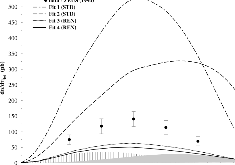
FIG. 3.: Rapidity distributions of jets from diffractive photoproduction processes. The labels indicate the respective Pomeron structure function and flux factor used in the calculation. The experimental data were measured by the ZEUS Collaboration [25].

FIG. 4.: Cross sections relative to diffractive photoproduction of jets in comparison to ZEUS data [25]. As in the other figures, the curve labels indicate the respective Pomeron structure function and flux factor used in the calculation.

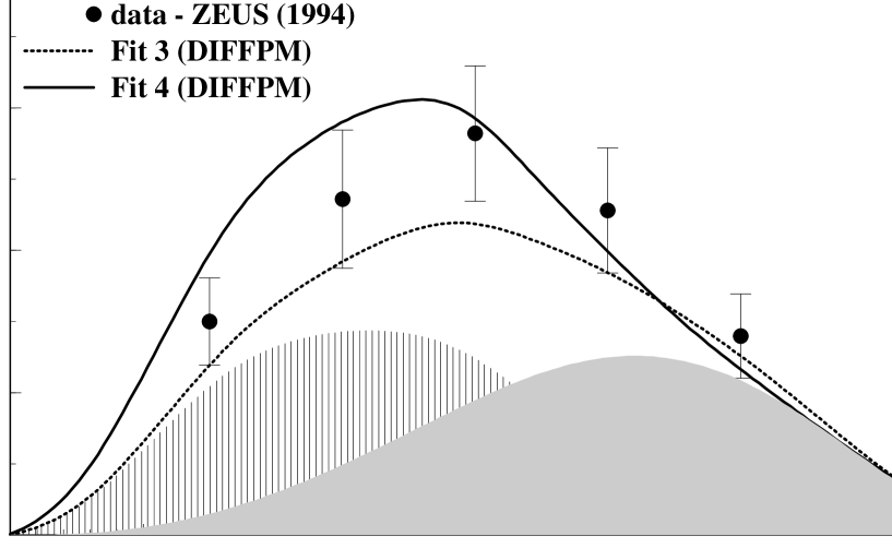
FIG. 5.: Rapidity distributions of jets from diffractive photoproduction processes. The labels indicate the respective Pomeron structure function used in the calculation, but with the redefinition discussed in the text. The experimental data were measured by the ZEUS Collaboration [25]. For the dotted curve, it is also shown its components: the direct contribution (hachured area) and resolved contribution (shaded area).

FIG. 6.: Cross sections relative to diffractive photoproduction of jets in comparison to ZEUS data [25]. The Pomeron structure function used in the calculations are the same as in Fig. 5.

		STD	STD	REN	REN
EXPERIMENT	RATE	Fit 1	Fit 2	Fit 3	Fit 4
($W$’s)		(hard-hard)	(free-delta)	(hard-hard)	(free-zero)
CDF (Rap-Gap)	$1.15\pm 0.55$	3.12	3.54	0.53	0.58

TABLE I.: Diffractive production rates of $W$’s (all values are given in percentages).

	(a)	(b)	(c)	(d)
EXPS.	CDF	CDF	D0	D0
	(Rap-Gap)	(Roman Pots)	(630 GeV)	(1800 GeV)
RATES	$0.75\pm 0.10$	$0.109\pm 0.016$	1-2	$0.67\pm 0.05$
(%)
rapidity	$-3.5<\eta<-1.8$	$-3.5<\eta<-1.8$	$-4.1<\eta<-1.6$	$-4.1<\eta<-1.6$
$x_{\tt I\!P}$	$x_{\tt I\!P}<0.1$	$0.05<x_{\tt I\!P}<0.1$	$x_{\tt I\!P}<0.1$	$x_{\tt I\!P}<0.1$
$E_{T_{min}}$	$20$ GeV	$10$ GeV	$12$ GeV	$12$ GeV

TABLE II.: Experimental data and respective kinematical cuts for different measurements of diffractive production of dijets.

		STD	STD	REN	REN
EXPERIMENTS	RATES	Fit 1	Fit 2	Fit 3	Fit 4
(JETS)		(hard-hard)	(free-delta)	(hard-hard)	(free-zero)
CDF (Rap-Gap)	$0.75\pm 0.10$	15.3	6.33	0.62	0.52
CDF (Roman Pots)	$0.109\pm 0.016$	3.85	1.13	0.15	0.16
D0 (630 GeV)	1-2	15.4	6.41	0.87	0.71
D0 (1800 GeV)	$0.67\pm 0.05$	16.6	6.14	0.65	0.57

TABLE III.: Diffractive production rates of dijets (all values are given in percentages).

REFERENCES

- [1] G. Ingelman and P. E. Schlein, Phys. Lett. B 152, 256 (1985).
- [2] UA8 Collaboration, R. Bonino it et al., Phys. Lett. B 211, 239 (1988).
- [3] P. Schlein [for the UA8 Collab.], “The Evidence for Partonic Behavior of the Pomeron”, Proceedings of the International Europhysics Conference on High Energy Physics - Marseille, France, 22-28 July 1993 (Editions Frontieres - ed. J. Carr and M. Perrottet) p. 592.
- [4] P. Bruni and G. Ingelman, Phys. Lett. B 311, 317 (1993).
- [5] L. Alvero et al., “Diffractive Production of Jets and Weak Bosons and Tests of Hard-Scattering Factorization”, preprint PSU/TH/177, hep-ph/9805268.
- [6] H1 Collaboration, T. Ahmed et al., Phys. Lett. B 348, 681 (1995).
- [7] ZEUS Collaboration, M. Derrick et al., Zeit. Phys. C 68, 569 (1995).
- [8] H1 Collaboration, C. Adloff et al., Zeit. Phys. C 76, 613 (1997).
- [9] R. J. M. Covolan and M. S. Soares, Phys. Rev. D 57, 180 (1998).
- [10] A. Donnachie and P. V. Landshoff, Nucl. Phys. B 303, 634 (1988).
- [11] K. Goulianos, Phys. Lett. B 358, 379 (1995).
- [12] T. Gehrmann and W. J. Stirling, Zeit. Phys. C 70, 89 (1996).
- [13] K. Golec-Biernat and J. Kwieciński, Phys. Lett. B 353, 329 (1995).
- [14] Yu. L. Dokshitzer, Sov. Phys. JETP 46, 641 (1977); V. N. Gribov and L. N. Lipatov, Sov. J. Nucl. Phys. 15, 438, 675 (1972); G. Altarelli and G. Parisi, Nucl. Phys. B 126, 298 (1977).
- [15] CDF Collaboration, F. Abe et al., Phys. Rev. Lett. 78, 2698 (1997).
- [16] H. Baer and M. H. Reno, Phys. Rev. D 43, 2892 (1991).
- [17] W. T. Giele, E. W. N. Glover, D. A. Kosower, Nucl. Phys. B 403, 633 (1993).
- [18] U. Baur, T. Han and J. Ohnemus, Phys. Rev. D 48, 5140 (1993).
- [19] W. Greiner and J. Reinhardt, “Quantum Electrodynamics”, 2nd edition, Springer-Verlag, Berlin, Heidelberg - Germany (1994).
- [20] M. Gluck, E. Reya, A. Vogt, Zeit. Phys. C 67, 433 (1995).
- [21] M. Gluck, E. Reya, A.V ogt, Phys. Rev. D 46, 1973 (1992).
- [22] CDF Collaboration, F. Abe et al., Phys. Rev. Lett. 79, 2636 (1997).
- [23] M. G. Albrow (for the CDF Collab.), published in the Proceedings of the VII Blois Workshop on Elastic and Diffractive Scattering - Recent Advances in Hadron Physics, Seoul, Korea, June 10-14 (1997).
- [24] D0 Collaboration, S. Abachi et al., paper presented at the 28th Int. Conf. on High Energy Physics (ICHEP 96), Warsaw, Poland (July 1996).
- [25] ZEUS Collaboration, J. Breitweg et al., Eur. Phys. J. C 5, 41 (1998).
- [26] G. Abbiendi, Riv. N. Cimento 20, 4 (1997).
- [27] K. Goulianos and J. Montanha, Factorization and Scaling in Hadronic Diffraction, Rockefeller University preprint: RU 97/E-43; hep-ph/9805496.
- [28] Chung-I Tan, “Diffractive Production at Collider Energies I: Soft Diffraction and Dino’s Paradox”, Brown University preprint: BROWN-HET-1082 (1997), hep-ph/9706276.
- [29] S. Erhan and P. Schlein, Phys. Lett. B 427, 389 (1998).
- [30] E. Gotsman, E. Levin, and U. Maor, A Two Channel Calculation of Screening Corrections, Tel Aviv University preprint: TAUP 2560 (1999); hep-ph/9901416.